Abstract
In view of the fact that indoor positioning systems are usually affected by non-Gaussian noise in complex indoor environments, this paper tests the data in the actual scene and analyzes the distribution characteristics of noise, and proposes a new indoor positioning algorithm based on maximum correntropy unscented information filter (MCUIF). The proposed indoor positioning algorithm includes three steps: First, the estimation of the state matrix and the corresponding covariance matrix are predicted through the unscented transformation (UT). Second, the observed information is reconstructed by using a nonlinear regression method on the basis of the maximum correntropy criterion (MCC). Third, the contribution of information vector is gained by non-Gaussian measurement and the predicted information vector is corrected by the contribution of information vector. Finally, the gain of information filtering is got by the information entropy state matrix and the information entropy measurement matrix to calculate the position coordinates of the unknown nodes. This algorithm enhances the robustness of the MCUIF to non-Gaussian noise in complex indoor environments. The results from the indoor positioning experiments show that MCUIF is better than the traditional methods in state estimation and position location of the unknown nodes.
1. Introduction
In recent years, with the gradual increase in the demand, indoor positioning has been applied in medical centers, smart homes, shopping malls, underground mine personnel location tracking, cargo tracking, and other fields. At present, both visual positioning technology and wireless positioning technology are hotspots in indoor positioning research [1,2,3]. Visual positioning technology is more widely used in autonomous positioning and the navigation of robots and unmanned aerial vehicles [4,5]. Visual positioning has a very prominent advantage and does not need to carry a signal source or remote control. However, the shortcomings are also obvious: the image processing volume is huge, the general computer cannot complete the calculation, and the real-time performance is poor; it is limited by the light conditions and cannot work in dark environments. Compared with visual positioning, wireless positioning technology is not affected by light and has low environmental requirements. The RSS-based wireless indoor positioning system received widespread attention as soon as it first appeared due to its advantage of not requiring specific hardware. Because of the huge application scenario and high commercial value of indoor positioning [6], scholars have studied many excellent positioning algorithms for indoor positioning systems [6,7,8]. The commonly used estimation algorithms [9,10] are Angle of Arrival (AOA) [11], Received Signal Strength (RSS) [12], Time of Arrival (TOA) [13], Time Difference of Arrival (TDOA) [14], and some mixed algorithms. Kalman filter, as an optimal state estimation algorithm, has been introduced into indoor positioning and achieved good results. In addition, there are some improved Kalman filter algorithms such as Extended Kalman Filter (EKF) [15,16,17], Unscented Kalman filter (UKF) [18,19], Cubature Kalman Filter (CKF) [20,21], etc. The work in [15] applied wireless sensor network positioning with extended Kalman filter (EKF). The work in [17] proposes an localization algorithm based on EKF by edge computing, and its location landmark has been update in a mobile robot. The work in [22] designs a mobile target location and tracking algorithm based on square root unscented kalman filter (SR-UKF) in the Internet of Things environment. Compared with the traditional EKF and UKF algorithms in the indoor positioning system, this algorithm has obtained lower positioning and tracking errors with the same computational complexity. The authors of [23] propose a filtering method via Kalman filter for the speed and direction of the indoor robots.
The algorithms in the above documents [15,17,22,23] are assumed that the observation noise is Gaussian noise. However, in the actual complex indoor environment, radio frequency signals are prone to reflection, diffraction, and refraction. At the same time, changes in the surrounding environment such as temperature, humidity, obstacles, and non-line-of-sight will also cause certain effects on the propagation of radio frequency signals. These factors cause indoor positioning systems to be usually affected by multi-peak heavy-tailed non-Gaussian noise [24]. The accuracy of the Kalman filter based on the MMSE criterion will be significantly reduced, and even cause filter scattering. Therefore, in the practical application of indoor positioning, the research on non-Gaussian noise becomes very meaningful. In order to solve the positioning estimation problem in such noise, by combining MCC and UIF, we propose an indoor positioning algorithm in view of MCUIF [25,26,27,28,29,30], and given the indoor positioning system, MCUIF enhances the robustness of UIF and achieves better performance than the traditional UKF and EKF.
The structure of this paper about MCUIF is as below. In Section 2, we briefly explain the process model and the measurement model. Moreover, we collect the signal strength between the unknown nodes and the known nodes in the actual scene, then adopt Kolmogorov–Smirnov to test and analyze the distribution characteristics of RSS noise. Next, the maximum entropy criterion is introduced, and the indoor location algorithm based on MCUIF is derived in Section 3. Then, in Section 4, we describe the field scenario experiments, and the experimental results show the excellent performance of MCUIF. Finally, Section 5 gives a conclusion.
2. Process and Measurement Models
2.1. Process Model
Assume that L wireless Access Point(AP) nodes are set in the indoor scene, and the coordinate of the l-th AP is . The moving unknown node can receive the signal strength from the APs. The position and velocity of the moving unknown node are described as the state . Its motion can be described by [31]
It can also be abbreviated as
where , where represents the process noise and its covariance matrix is . If we set as the sampling interval and the total running time as 50 s, the total number of acquisitions is times.
2.2. Measurement Model
RSS ranging technology is also known as signal strength ranging method, which is calculated based on the radio propagation path loss model [31]. In complex and changeable indoor environment, traditional wireless signal transmission models are no longer applicable. Currently, the more commonly used models are logarithmic distance path loss models, which have been verified in various real environments. The general model is [32]
where represents the received signal strength indication (RSSI) value received at from the transmitting nodes. The measured value is generally a negative value, and the absolute value of which is taken in the calculation. represents the RSSI value received from the transmitting nodes, also known as the reference fading RSSI value, where calls as the reference distance is generally taken as 1 meter. The path dynamic fading index indicates that the signal increases with the transmission distance. The attenuation speed of the signal power is fading if the transmission distance increases. This value depends on the transmission environment and the type of field environment. is the signal strength noise. In indoor positioning, the RSSI can be extracted from the transceiver of the mobile nodes. We adopt the logarithmic distance path loss model as the measurement model for predicting RSSI. is the weighted average of the signal strength measured multiple times from the i-th known node, as follows:
where is the j-th signal strength between the measured and the i-th AP. To enhance the anti-interference ability of the indoor positioning system against other external wireless radios, it is taken as the observation . That is,
where and is the observation noise built by the mixed Gaussian model, its covariance matrix is . is the coordinate vector of the L-th known node, and is the coordinate vector of the k-th moment of the moving unknown node. is the operator about the Euclidean distance between unknown nodes and known nodes.
The actual indoor scene is shown in Figure 1. We use a CC2530-based Zigbee indoor positioning system to test the signal strength from unknown nodes to known nodes and analyze its noise characteristics. The experimental scene shown in Figure 1a is the corridor on the fifth floor of the experimental building of Henan University of Technology. There are obstacles and moving pedestrians in the corridor. The tested CC2530-based Zigbee indoor positioning system has a coordinator, a test node, and four APs. The test node and the PC are connected through a coordinator. The four APs are AP1, AP2, AP3, and AP4; they are distributed as shown in Figure 1 and the coordinates of the APs have been determined. They are known nodes and can be used as the transmitter and receiver of wireless signals. The test node is a mobile unknown node. The signal strength of other nodes received by the test node is transmitted to the coordinator, the coordinator node is connected with the computer, the coordinator then transmits the received data to the computer, the computer stores the data, and then calculates and determines the coordinates of the test node. In the test experiment, the unknown node is resting state, the signal strength data is collected by PC at rest for 3 min for each node each time, and 50 sets of data are selected among them. The data sets are checked and analyzed for the error distribution characteristics of four APs signals received by unknown nodes.
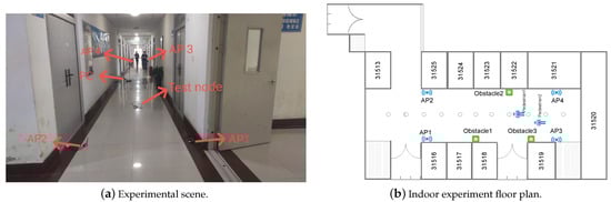
Figure 1.
The scene and floor plan of the indoor positioning experiment. The wireless icon marks the location of the AP node, the small circle is the trajectory of the test node along the corridor, the green ones are the obstacles, and the small person is the walking pedestrian.
The experimental results of the tests are shown in Figure 2. With the experimental results of the Kolmogorov–Smirnov [33,34,35,36] test analysis, if the test rejects the null hypothesis at significant level, the signal strengths from the unknown nodes to the four APs have a non-Gaussian distribution.
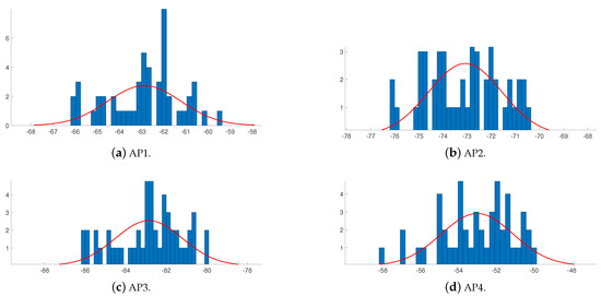
Figure 2.
Error distribution of the signal strength collected from APs.
Therefore, as shown in Figure 2, the signal strength of the APs received by the unknown node shows a non-Gaussian distribution, and then the ranging errors between the unknown nodes and the known APs are also non-Gaussian noise. However, the current methods such as the algorithms in [15,17,22,23] are aimed at the noise of Gaussian. In this paper, for such non-Gaussian indoor positioning problem, we consider the dimension of the observation vector is smaller than the dimension of the state vector, and we have designed a class MCUIF with relatively low computational complexity. Then, the signal intensity distribution is consistent with the superposition of several Gaussian distributions, and the signal intensity distribution is fitted by the mixed Gaussian model. The proposed MCUIF positioning algorithm is calculated according to such distribution.
3. Related Work
3.1. Maximum Correntropy Criterion
Assume and are random variables and define the correlation entropy between and [27,28], which is expressed as
where is the kernel function and E is the expected operation symbol.
The kernel function based on maximum correntropy is usually selected as the Gaussian one:
where is the kernel width, and and are the elements of random variables and , respectively.
Assuming that the function of joint distribution between and is expression of , then the correntropy is expressed as
In the practical complex indoor positioning application environment, the data volume is usually limited, and the function of joint distribution between and is usually unknown, the correntropy has been estimated through the average estimator of the finite sample:
where , and i is the i-th sampling point of the function , and M is a feasible set of parameters.
3.2. Location Algorithm Based on MCUIF
The MCUIF algorithm reconstructs the observation information is based on the nonlinear regression method of MCC. Such an algorithm enhances the robustness of UIF to non-Gaussian noise. The algorithm regarding the proposed indoor positioning is applied to the state estimation of the indoor localization nodes, and the problem of the influence of heavy-tailed non-Gaussian noise in indoor localization is solved. According to Equations (1) and (5), the nonlinear discrete-time system model for indoor positioning is
where represents the state vector of the unknown node, represents the observation vector of the indoor positioning network system. and , representing the nonlinear functions of the system and the observation, respectively, are assumed to be continuously differentiable.
Then, the MCUIF filtering algorithm based on maximum correntropy has two main parts of the state time updating and the measurement updating, and is specifically derived as follows:
- State Time UpdatingFirst, according to the UT transformation and formulas (12) and (13), a set of sampling points (called Sigma point set) has been calculated:where k is the state dimension, is a scaling parameter, and , means the i-th column of the square root of the matrix.Next, the corresponding weights of these sampling points have been obtained:where is a non-negative weighting factor and describes the distribution status of sampling points.Then, the set of 2k + 1 Sigma points is formed according to the system equation:Then, the prediction and covariance matrix of the system state quantities are, respectively, as follows:andThen, the matrix about Fisher information is expressed asand the information state of information filtering is expressed as
- Measurement UpdatingAccording to the predicted value of one step, the UT transformation is used again to generate a new Sigma point set:The predicted new Sigma point set is substituted into the observation Equation (10) to obtain the corresponding observed Sigma point set:The predicted observed values of the observation Sigma point set are obtained according to step (3), and then the predicted mean values of the indoor positioning system are obtained by weighted summation as follows:Combining Equations (10) and (11) with Equations (15) and (18), we obtain the following nonlinear model:with , and .Through the derivation of MCC, formula (25) can be obtained. See Appendix A for the detailed derivation process. Then, the modified covariance iswhere ,, .However, the true state is unknown in practice indoor environment. Suppose , that is, in Equation (A2), then we get and the modified observation covariance is . Then, the covariance of the systematic observation isand the covariance matrix isThen, the information state contribution is calculated asand the corresponding information matrix is obtained asFinally, the information state vector and the Fischer information matrix are calculated:
4. Experiment and Simulation Analysis
4.1. Validity Analysis of MCUIF Method
In the experimental positioning scenario shown in Figure 1, we randomly selected 9 Testing Nodes (TNs) and placed the positioning tags at TNs in turn for 2 min, collected the signal strength data, and used different positioning algorithms of LS, EKF, UIF, and MCUIF to calculate the positioning coordinates of each reference node; the path dynamic attenuation index is . In the LS, EKF, and UIF algorithms, assume that the observed noise is Gaussian noise conforming to the normal distribution, and set the observed noise variance . The positioning accuracy is measured by the Root Mean Square Error (RMSE) of each reference node:
where represents the amount of TNs, and and represent the estimated position coordinates and actual position coordinates of the unknown nodes, respectively.
In order to base the experimental conclusions on a more scientific and reliable basis and avoid simplification and absoluteness, we use the significance T test method in statistical theory for testing. As the MCUIF and LS two sets of test data in this experiment belong to the independent sample T test, t can be calculated according to the following formula:
where and are the average values measured by MCUIF and LS, respectively, and is the standard deviation of the difference between the average value measured by MCUIF and LS.
If the number of two samples is the same, the formula for calculating the standard deviation of the difference between the averages of the two samples is
where , are the standard deviations of MCUIF and LS tests, respectively, and n is the number of MCUIF and LS measurement data, respectively.
The relevant data of MCUIF and LS tests are shown in the Table 1.

Table 1.
Sample statistics.
In this T test, we assume the null hypothesis is and alternative hypothesis is . The difference between the averages of the two samples of MCUIF and LS is
From the t distribution table, it can be obtained that . Now, calculate according to the formula (32), and the result falls in the negative domain. Therefore, the alternative hypothesis can be rejected, which means that at the significance level of , the MCUIF algorithm is better than the LS method. In turn, the significance T test method can be used; therefore, it can also be verified that the MCUIF algorithm is better than the EKF algorithm and the UIF algorithm when the confidence is taken as . The test proves that the experimental result is statistically significant when the current measurement value or more of the measurement value is measured.
The RMSE results calculated by each different algorithm are shown in Figure 3. In the LS, EKF, and UIF algorithms shown in Figure 3, the observation noise is assumed to be Gaussian noise conforming to the normal distribution. As can be seen from Figure 3, by the MCUIF-based indoor positioning algorithm, the maximum value of RMSE for each reference point is m, the minimum value is m, and the average value is m, which is smaller than the RMSE of LS, EKF, and UIF indoor positioning, and has high positioning accuracy at the significance level of .
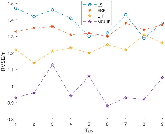
Figure 3.
Comparison on positioning accuracies of different location algorithms.
As shown in Figure 3, the LS, EKF, and UIF algorithms assume that their noise is Gaussian distribution. Due to the introduction of maximum correlation entropy, MCUIF compared with other positioning algorithms shows that due to the use of Gaussian mixture model to fit noise, which is closer to the actual situation, MCUIF has lower requirements for the distribution characteristics of observation noise, and it can also perform better on observation data under non-Gaussian conditions. With filtering processing, the positioning accuracy has been significantly improved, especially when the positioning errors of other algorithms are large, the accuracy of the MCUIF positioning algorithm is more obvious. Therefore, the MCUIF positioning algorithm is more robust than other algorithms and has the stronger ability to adapt to the environment.
4.2. Analysis of MCUIF Method Robustness
The research algorithm is more in line with the real application environment in the location of multiple pedestrians, and it is of great significance for evaluating the robustness of the algorithm. The experiment site is still selected on the corridors in the experimental site as shown in Figure 1, because there are often pedestrians walking in the corridors. In five different working days, a total of 300 test samples were collected under the condition of pedestrians walking back and forth for position estimation, and the average error distance of the positioning results of several algorithms was compared. The comparison of the average error distance of the algorithm in a multi-pedestrian environment is shown in Table 2. Compared with the ALE in Figure 3, the performance of each algorithm has decreased. Among them, the performance degradation of the LS algorithm and EKF algorithm is more significant. The average error of the UIF algorithm and MCUIF algorithm also increased by and , respectively. Nevertheless, the average error distance of the UIF algorithm remains within 1.5 m, which is basically acceptable.
Table 2.
Comparison ALE of different algorithms in multiple pedestrian walking environments.
In the simulation process, the Averaged Localization Error (ALE) is used to compare various positioning methods; ALE is defined as
The smaller the ALE estimated for the unknown node position, the higher the accuracy of the characterization estimation.
4.3. Experimental Analysis of the Corner
There are many corners in the teaching building, and we have done experimental analysis specifically for the corners. The test results show that the placement of the AP at the corner is closely related to its positioning accuracy. For Scheme I, we placed APs as shown in Figure 4a; the AP1-4 placed on one side of the corridor corner remained unchanged, and two APs were placed on the other side of the corridor corner: AP5 and AP6; Scheme II, as shown in Figure 4b, AP1-6 is placed in the same location as in scheme I, we add AP7 at the key points of the corner, and the positioning accuracy is significantly improved. The RMSE of its positioning is shown in Table 3. As shown in Table 3, at the curve, in the second scheme, the performance of the four algorithms of LS, EKF, UIF and MCUIF has been significantly improved. Four points were selected for testing before and after the corner, a total of 8 points, the average mean square error of the test results is shown in Table 3. The average error of the UIF algorithm and the MCUIF algorithm of scheme II and scheme I is also reduced and , respectively.
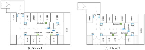
Figure 4.
Positioning experiment of placing AP at the corner.
Table 3.
The ALE of AP placement at the corner.
4.4. Simulation Analysis to Select the Appropriate Kernel Bandwidth
In the actual complex indoor environment, the positioning accuracy is often affected by non-Gaussian noise, which will cause the accuracy of traditional nonlinear filtering algorithms to decrease or even diverge. Therefore, it is necessary to study the nonlinear robust filtering algorithm for non-Gaussian noise, and the method proposed introduces the maximum correntropy based on UIF, which makes the filtering robust against non-Gaussian.
The following is a specific simulation experiment comparing and analyzing the selection of the appropriate kernel bandwidth. As shown in Figure 5, four APs are deployed in the indoor localization area, whose corresponding coordinates are A1(0,0), A2(0,10), A3(10,0), and A4(10,10). Assuming that the state vector of the unknown node in the experiment is shown in Equation (1), the initial real state is provided by LS (position unit m, velocity unit m/s) , the initial estimation of state noise covariance matrix is set to , and the initial covariance matrix of the process noise is . The observed non-Gaussian noise is comprehensively analyzed by the measured signal strength, and it is obtained as .
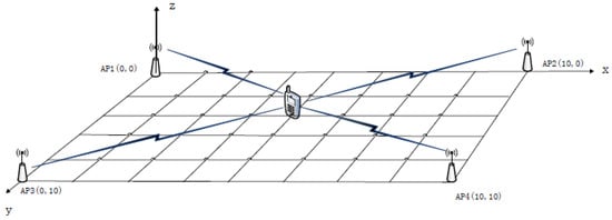
Figure 5.
Node location diagram.
In order to find the best kernel bandwidth, four different kernel bandwidths are selected first for experiment, and the kernel bandwidths are set to , , , and , respectively. The experimental results are shown in Figure 6, Figure 7 and Figure 8.
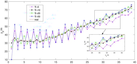
Figure 6.
Dynamic localization with different kernel bandwidths.
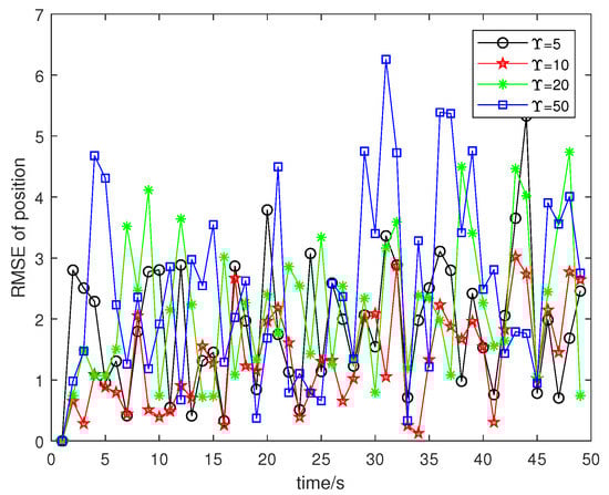
Figure 7.
RMSE of Position.
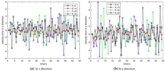
Figure 8.
Error curve of velocity estimation.
Based on the analysis of the above simulation experiments, Figure 6 shows the comparison of the dynamic positioning of the MCUIF algorithm in the four kernel bandwidths, and Figure 7 is the comparison of the positioning RMSE in the four kernel bandwidths. Figure 8a is the velocity estimation error of the unknown nodes in the x direction, and Figure 8b is the velocity estimation error of the unknown node in the y direction.
The analysis of Figure 6, Figure 7 and Figure 8 and Table 4 shows that when MCUIF selects the kernel bandwidth, the positioning accuracy after filtering by MCUIF is the highest and the performance effect is the best. Based on the analysis in Figure 6, Figure 7 and Figure 8 and Table 4, when MCUIF selects the kernel bandwidth, the positioning accuracy after the filtering of MCUIF is the highest, and the performance effect is the best.
Table 4.
Simulation results of MCUIF for four different kernel bandwidths.
5. Conclusions
This paper has mainly studied and analyzed the indoor positioning problem when the measured noise is non-Gaussian and has proposed an indoor positioning method based on MCUIF. Indoor positioning experiments have been carried out on the indoor positioning method based on the LS, EKF, UIF, and MCUIF indoor positioning methods proposed. The indoor positioning experimental results have shown that the alignment accuracy of the indoor positioning method based on LS, EKF, and UIF is lower than the proposed MCUIF method. Moreover, the indoor positioning method based on MCUIF under four different kernel bandwidths has been analyzed, and it has been concluded that the proposed MCUIF-based method has the best effect when . In summary, the experiments and analysis show that the MCUIF-based indoor positioning method can better accomplish indoor positioning with non-Gaussian noise in the measurement noise, and the positioning accuracy is higher than that of LS, EKF, and UIF indoor positioning methods.
The method proposed in this paper can be used for autonomous navigation of wheeled robots. Inertial measurement unit (IMU), wireless positioning technology, vision, etc. can be used for autonomous navigation of wheeled robots. At present, IMU, wireless positioning technology, and vision have their own advantages and disadvantages. IMU will have cumulative errors, and visual navigation will be limited to factors such as light. If wireless positioning technology can be combined with visual positioning, IMU, etc. for fusion positioning, autonomous navigation of wheeled robots will be more widely used. Therefore, our next step is to study the application of MCUIF-based wireless positioning technology, vision, and IMU fusion positioning in autonomous navigation of wheeled robots.
Author Contributions
This paper is a collaborative work by all authors. Li Ma and Xiaoliang Feng conceived and designed the main idea and experiments. Li Ma performed the experiments and wrote the paper. Ning Cao and Minghe Mao provided important and guiding suggestions, supported the paper and gave support for the cognitive experiment. All authors have read and agreed to the published version of the manuscript.
Funding
This research was funded by the National Natural Science Foundation of China under Grant (61701167).
Institutional Review Board Statement
Not applicable.
Informed Consent Statement
Not applicable.
Data Availability Statement
Some or all data, models, or code that support the findings of this study are available from the corresponding author upon reasonable request.
Conflicts of Interest
The authors declare no conflict of interest.
Appendix A
Conducting Cholesky decomposition of the covariance matrix and the joint matrix of from formula (24), we get
Both sides of Equation (A1) are left multiplied by , due to , then the following equation is obtained:
then, where , , and
.
As , the residual error are white. Then, the element in the j-th row of is
According to the properties of correntropy, the cost function is
where denotes the dimension and the j-th element of , denotes the j-th row of , and, where the kernel bandwidth is .
If the function is maximized, the optimal estimation of the state can be obtained. Then, the optimal estimation value satisfies
Let
that is
From the properties of related entropy, it can also be written as
Therefore, it can be seen that
References
- Deng, Z.; Yin, L.; Tang, S.; Liu, Y.X.; Song, W.X. A Survey of Key Technology for Indoor Positioning. Navig. Position. Timing 2018, 5, 14–22. [Google Scholar]
- Malik, D.; Chinthaka, P. Development of an Automated Camera-Based Drone Landing System. IEEE Access 2020, 11, 202111–202121. [Google Scholar]
- Alhomayani, F.; Mahoor, M.H. Deep learning methods for fingerprint-based indoor positioning: A review. J. Locat. Based Serv. 2020, 14, 129–200. [Google Scholar] [CrossRef]
- Chinthaka, P.; Dang, N.H.T.; Tomotaka, K.; Hiroharu, K. Improved Method for Horizontal Movement Measurement of Small Type Helicopter Using Natural Floor Features. In Proceedings of the Joint Conference of the International Workshop on Advanced Image Technology (IWAIT) and the International Forum on Medical Imaging in Asia (IFMIA), Tainan, Taiwan, 11–13 January 2015. [Google Scholar]
- Chinthaka, P.; Masashi, M.; Ryo, G.; Takao, N.; Kiyotaka, K. Improving landmark detection accuracy for self-localization through baseboard recognition. Int. J. Mach. Learn. Cybern. 2017, 8, 1815–1826. [Google Scholar]
- Johannes, W.; Thomas, J.; Christian, S. Self-localization based on ambient signals. Theor. Comput. Sci. 2012, 453, 98–109. [Google Scholar]
- Murata, S.; Chokatsu, Y.; Kazumasa, K.; Shigenori, I.; Hiroshi, T. Accurate indoor positioning system using near-ultrasonic sound from a smartphone. In Proceedings of the 2014 Eighth International Conference on Next Generation Mobile Apps, Services and Technologies, Oxford, UK, 10–12 September 2014. [Google Scholar]
- Wang, Y.; Ren, W.; Cheng, L.; Zou, J. A Grey Model and Mixture Gaussian Residual Analysis-Based Position Estimator in an Indoor Environment. Sensors 2020, 20, 3941–3942. [Google Scholar] [CrossRef]
- Long, C.; Yifan, L.; Mingkun, X.; Yan, W. An Indoor Robust Localization Algorithm Based on Data Association Technique. Sensors 2020, 20, 6598. [Google Scholar]
- Tianfei, C.; Lijun, S.; Ziqiang, W.; Yao, W.; Zhipeng, Z.; Pan, Z. An enhanced nonlinear iterative localization algorithm for DV-Hop with uniform calculation criterion. Ad Hoc Netw. 2021, 111, 102327. [Google Scholar]
- Slavisa, T.; Marko, B.; Rui, D.; Milan, T.; Nebojsa, B. Bayesian methodology for target tracking using combined RSS and AoA measurements. Phys. Commun. 2017, 25, 158–166. [Google Scholar]
- Tomic, S.; Marko, B.; Rui, D. RSS-based localization in wireless sensor networks using convex relaxation: Noncooperative and cooperative schemes. IEEE Trans. Veh. Technol. 2014, 64, 2037–2050. [Google Scholar] [CrossRef] [Green Version]
- Tomic, S.; Marko, B. Exact robust solution to TW-ToA-based target localization problem with clock imperfections. IEEE Signal Process. Lett. 2018, 25, 531–535. [Google Scholar] [CrossRef] [Green Version]
- Zhang, L.; Zhang, T.; Shin, H.S. An Efficient Constrained Weighted Least Squares Method with Bias Reduction for TDOA-Based Localization. IEEE Sens. J. 2021, 99, 10122–10131. [Google Scholar] [CrossRef]
- Masazade, E.; Fardad, M.; Varshney, P.K. Sparsity-promoting extended Kalman filtering for target tracking in wireless sensor networks. IEEE Signal Process. Lett. 2012, 19, 845–848. [Google Scholar] [CrossRef]
- Chuanyang, W.; Houzeng, H.; Jian, W.; Hang, Y.; Deng, Y. A robust extended Kalman filter applied to ultrawideband positioning. Math. Probl. Eng. 2020, 5, 1–12. [Google Scholar]
- Ullah, I.; Qian, S.; Deng, Z.; Lee, J.H. Extended Kalman Filter-based localization algorithm by edge computing in Wireless Sensor Networks. Digit. Commun. Netw. 2020, 7, 187–195. [Google Scholar] [CrossRef]
- Zhao, M.; Yu, X.L.; Cui, M.L.; Wang, X.G.; Wu, J. Square Root Unscented Kalman Filter Based on Strong Tracking. In Proceedings of the Third International Conference on Communications, Signal Processing, and Systems, Tianjing, China, 23 October 2015; Volume 1, pp. 797–804. [Google Scholar]
- Wang, X.; Fu, M.; Zhang, H. Target tracking in wireless sensor networks based on the combination of KF and MLE using distance measurements. IEEE Trans. Mob. Comput. 2011, 11, 567–576. [Google Scholar] [CrossRef] [Green Version]
- Liu, Y.; Jun, F.S.; Ming, Q.Z. The Location Algorithm Based on Square-Root Cubature Kalman Filter. Appl. Mech. Mater. 2013, 325, 1525–1529. [Google Scholar] [CrossRef]
- Feng, X.; Feng, Y.; Zhou, F.; Ma, L.; Yang, C.X. Nonlinear Non-Gaussian Estimation Using Maximum Correntropy Square Root Cubature Information Filtering. IEEE Access 2020, 8, 181930–181942. [Google Scholar] [CrossRef]
- Guo, J.; Zhang, H.; Sun, Y.; Bie, R. Square-root unscented Kalman filtering-based localization and tracking in the Internet of Things. Pers. Ubiquitous Comput. 2014, 18, 987–996. [Google Scholar] [CrossRef]
- Lu, J.Y.; Li, X. Robot indoor location modeling and simulation based on Kalman filtering. EURASIP J. Wirel. Commun. Netw. 2019, 1, 1–10. [Google Scholar] [CrossRef] [Green Version]
- Liu, W.; Pokharel, P.P.; Principe, J.C. Correntropy: Properties and applications in non-Gaussian signal processing. IEEE Trans. Signal Process. 2007, 55, 5286–5298. [Google Scholar] [CrossRef]
- Fan, Y.; Zhang, Y.; Wang, G.; Wang, X.; Li, N. Maximum correntropy based unscented particle filter for cooperative navigation with heavy-tailed measurement noisese. IEEE Access 2020, 8, 70162–70170. [Google Scholar]
- Wang, G.; Li, N.; Zhang, Y. Maximum correntropy unscented Kalman and information filters for non-Gaussian measurement noise. J. Frankl. Inst. 2017, 354, 8659–8677. [Google Scholar] [CrossRef]
- Liu, X.; Chen, B.; Zhao, H.; Qin, J.; Cao, J. Maximum correntropy Kalman filter with state constraints. IEEE Access 2017, 5, 25846–25853. [Google Scholar] [CrossRef]
- Chen, B.; Liu, X.; Zhao, H.; Principe, J.C. Maximum correntropy Kalman filter. Automatica 2017, 76, 70–77. [Google Scholar] [CrossRef] [Green Version]
- Guo, Y.; Wu, M.; Tang, K.; Zhang, L. Square-Root Unscented Information Filter and Its Application in SINS/DVL Integrated Navigation. Sensors 2018, 18, 2069. [Google Scholar] [CrossRef] [Green Version]
- He, J.; Sun, C.; Zhang, B.; Wang, P. Maximum correntropy square-root cubature Kalman filter for non-Gaussian measurement noise. In Proceedings of the IEEE International Conference on Network Infrastructure and Digital Content, Guilin, China, 17–19 November 2013; Volume 39, pp. 1543–1554. [Google Scholar]
- Heinemann, A.; Gavriilidis, A.; Sablik, T.; Stahlschmidt, C.; Velten, J.; Kummert, A. RSSI-Based Real-Time Indoor Positioning Using ZigBee Technology for Security Applications. In Proceedings of the International Conference on Multimedia Communications, Services and Security, Krakow, Poland, 11–12 June 2014. [Google Scholar]
- Tomic, S.; Beko, M.; Dinis, R.; Lipovac, V. RSS-based localization in wireless sensor networks using SOCP relaxation. In Proceedings of the 2013 IEEE 14th Workshop on Signal Processing Advances in Wireless Communications (SPAWC), Darmstadt, Germany, 16–19 June 2013. [Google Scholar]
- Mahjoub, H.N.; Tahmasbi-Sarvestani, A.; Gani, S.M.O.; Fallah, Y.P. Composite α-μ Based DSRC Channel Model Using Large Data Set of RSSI Measurements. IEEE Trans. Intell. Transp. Syst. 2018, 20, 205–217. [Google Scholar] [CrossRef]
- Gour, P.; Anil, S. Localization in wireless sensor networks with ranging error. Intell. Distrib. Comput. 2015, 10, 55–69. [Google Scholar]
- Rea, M.; Fakhreddine, A.; Giustiniano, D.; Lenders, V. Filtering noisy 802.11 time-of-flight ranging measurements from commoditized wifi radios. IEEE/ACM Trans. Netw. 2017, 25, 2514–2527. [Google Scholar] [CrossRef]
- Esfandiari, R.S. Numerical Methods for Engineers and Scientists Using MATLAB®, 2nd ed.; CRC Press: Boca Raton, FL, USA, 2017. [Google Scholar]
Publisher’s Note: MDPI stays neutral with regard to jurisdictional claims in published maps and institutional affiliations. |
© 2021 by the authors. Licensee MDPI, Basel, Switzerland. This article is an open access article distributed under the terms and conditions of the Creative Commons Attribution (CC BY) license (https://creativecommons.org/licenses/by/4.0/).