Article

Socioeconomic and Environmental Impacts on Regional Tourism across Chinese Cities: A Spatiotemporal Heterogeneous Perspective

1
State Key Laboratory of Oil and Gas Reservoir Geology and Exploitation, School of Geoscience and Technology, Southwest Petroleum University, Chengdu 610500, China
2
State Key Laboratory of Resources and Environmental Information System (LREIS), Institute of Geographic Sciences and Natural Resources Research, Chinese Academy of Sciences, Beijing 100101, China
3
HEOA Group, West China School of Public Health and West China Fourth Hospital, Sichuan University, Chengdu 610041, China
4
Institute for Healthy Cities and West China Research Center for Rural Health Development, Sichuan University, Chengdu 610041, China
*
Author to whom correspondence should be addressed.
These authors contributed equally to this paper.
ISPRS Int. J. Geo-Inf. 2021, 10(6), 410; https://doi.org/10.3390/ijgi10060410
Submission received: 29 April 2021 / Revised: 9 June 2021 / Accepted: 10 June 2021 / Published: 14 June 2021
(This article belongs to the Special Issue Geo Data Science for Tourism)

Abstract

:
Understanding geospatial impacts of multi-sourced drivers on the tourism industry is of great significance for formulating tourism development policies tailored to regional-specific needs. To date, no research in China has explored the combined impacts of socioeconomic and environmental drivers on city-level tourism from a spatiotemporal heterogeneous perspective. We collected the total tourism revenue indicator and 30 potential influencing factors from 343 cities across China during 2008–2017. Three mainstream regressions and an emerging local spatiotemporal regression named the Bayesian spatiotemporally varying coefficients (Bayesian STVC) model were constructed to investigate the global-scale stationary and local-scale spatiotemporal nonstationary relationships between city-level tourism and various vital drivers. The Bayesian STVC model achieved the best model performance. Globally, eight socioeconomic and environmental factors, average wage (coefficient: 0.47, 95% credible intervals: 0.43–0.51), employed population (−0.14, −0.17–−0.11), GDP per capita (0.47, 0.42–0.52), population density (0.21, 0.16–0.27), night-time light index (−0.01, −0.08–0.05), slope (0.10, 0.06–0.14), vegetation index (0.66, 0.63–0.70), and road network density (0.34, 0.29–0.38), were identified to have nonlinear effects on tourism. Temporally, the main drivers might have gradually changed from the local macro-economic level, population density, and natural environment conditions to the individual economic level over the last decade. Spatially, city-specific dynamic maps of tourism development and geographically clustered influencing maps for eight drivers were produced. In 2017, China formed four significant city-level tourism industry clusters (hot spots, 90% confidence), the locations of which coincide with China’s top four urban agglomerations. Our local spatiotemporal analysis framework for geographical tourism data is expected to provide insights into adjusting regional measures to local conditions and temporal variations in broader social and natural sciences.

1. Introduction

Tourism is an underlying industry that promotes the development of the global economy [1]. According to the World Travel & Tourism Council (WTTC), tourism contributed 10.3% (8.9 trillion US dollars) of global GDP and provided one-tenth of the total number of jobs (330 million positions) in 2019 before the pandemic [2]. Through developing the tourism industry, local governments can markedly improve the level of infrastructure construction, increase employment opportunities, improve people’s living conditions, and promote urban economic growth [3,4,5]. In addition, tourism development is a fundamental part of a sustainable development strategy, which is recognized as a green industry by the world due to its low energy consumption and light pollution characteristics in the development process [6].
Despite being one essential force promoting regional economy, regional tourism itself is greatly influenced by socioeconomic status [7,8], including GDP [8], employment status [9], personal income [10], health and hygiene [7], industrial production index [11] and social media [12]. Besides the socioeconomic condition, research also identified the notable role of the environment in affecting regional tourism [13,14,15], especially climatic conditions, such as temperature [16], precipitation [17], sunshine [18], and relative humidity [19]. Road infrastructure was also a critical environmental driver enhancing the tourism industry [20,21]. However, all these previous studies only adopted a limited number of factors. It is necessary to consider the comprehensive impacts on tourism by combining socioeconomic conditions with environmental conditions.
When investigating relationships between regional tourism and potential explanatory factors, an unrealistic assumption persistently embedded in previous literature was that the variables’ relationships were homogeneous, which had been defined as stationarity. For instance, non-spatial tourism studies using qualitative analysis [22], feasible generalized least square (FGLS) regression [19], linear and quantile regression [23], or logit regression [24] are regarded as global-scale analyses and also ignore the existence of spatial effects. Likewise, some geospatial tourism studies using the spatial regression models, such as the exploratory spatial data analysis (ESDA) [25] or spatial econometric models [26], are capable of incorporating spatial effects for intercept or residual but are still unable to estimate a set of space-scale coefficients to characterize the varying region-specific relationships between variables. Hence, a more reasonable assumption in the real world highlights the heterogeneous or varying impacts of explanatory variables on tourism development due to region-specific situations, especially for studies conducted across large domains at finer geospatial scales. Such spatially heterogeneous variables relationships are called spatial nonstationarity in the field of statistics. At present, the geographically weighted regression (GWR) [27] is frequently used in tourism research, aiming at exploring such spatial nonstationarity between tourism and various influencing factors [28,29]. However, to the best of our knowledge, no study has been conducted from the spatiotemporal integrated nonstationary perspective, to fully explore both socioeconomic and environmental drivers on regional tourism development.
In China, as the area of interest in this study, there has long been an issue of regional tourism development disparities [30], which obstructed regional tourism sustainability to some extent [31]. Although these geospatial disparities have been extensively discussed at a provincial-level scale [32] or city group scale [33], seldom have studies explored the city-specific disparities of regional tourism, especially over mainland China. Based on tourism connotations and tourism elements, Chinese scholars have established a comprehensive indicator framework of influencing the urban tourism industry from multiple dimensions. Socioeconomic and environmental aspects are also considered indispensable indicators reflective of regional tourism industry development [34]. However, no existing studies ever investigated the joint impacts of socioeconomic and environmental conditions on China’s city-level tourism from a spatiotemporal heterogeneous perspective, to provide evidence-based implications for assisting the formulation of tourism-related policies at governmental levels in a timely and effective manner.
In an attempt to find effective factors affecting regional tourism outcomes to provide tourism strategies tailored for specific local spatial conditions and changing temporal circumstances, we constructed an explanatory variable framework composed of 30 variables, including socioeconomic and environmental conditions. We explored spatiotemporal heterogeneous relationships between the regional tourism development and the multi-source explanatory factors from 2008 to 2017 across Chinese cities by employing the Bayesian spatiotemporally varying coefficients (STVC) model [35,36]. The establishment of such an explanatory variable framework in our study also served as a contributor to the current literature in this field in terms of improving the comprehensiveness of the existing research index system as well as adding novel perspectives into this field based on the consideration of both spatial and temporal heterogeneity.

2. Materials and Methods

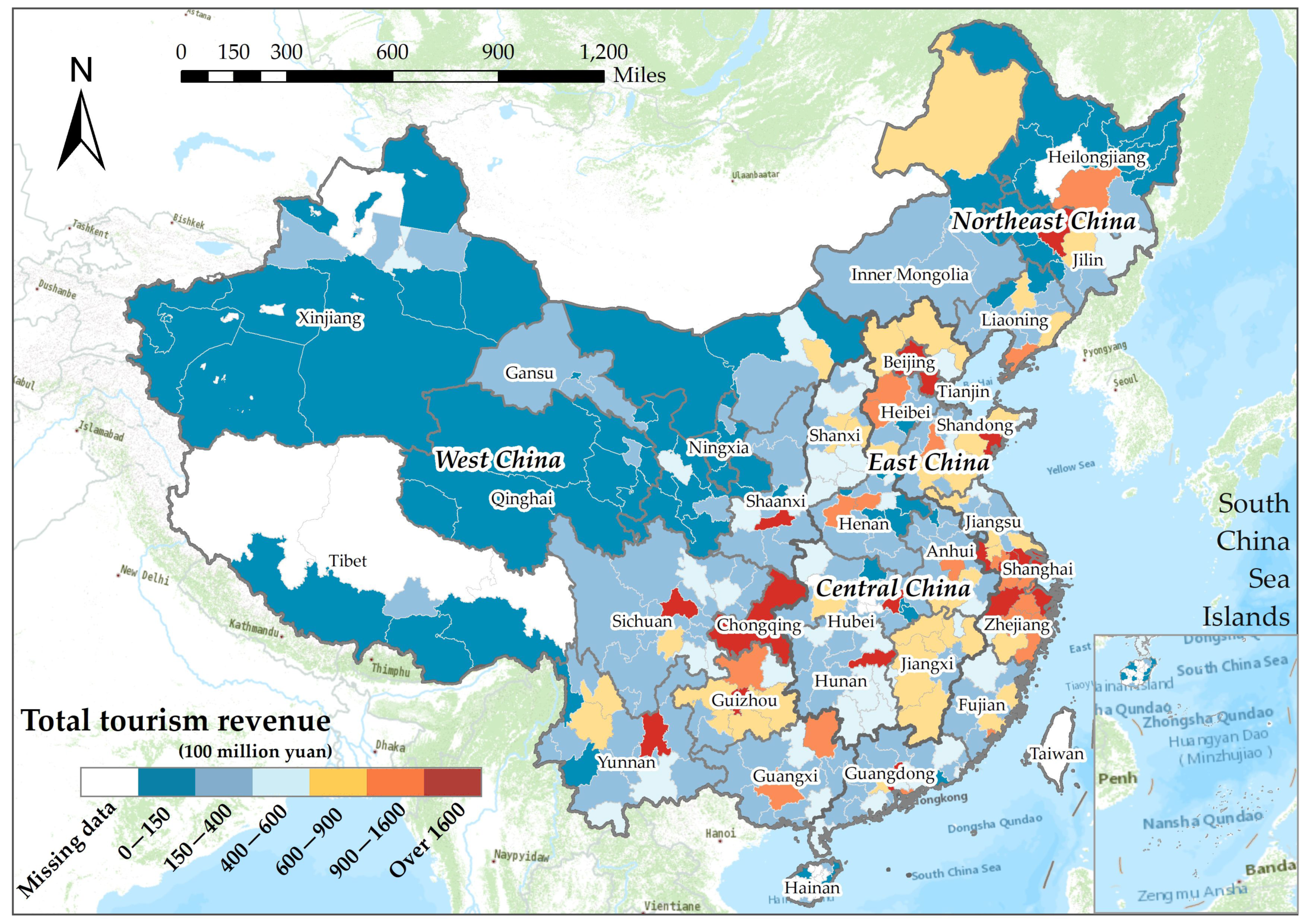
2.1. Study Area and Data

Considering the unbalanced development speed and regional differences in China’s tourism industry during the last decade, in this study, 343 prefecture-level areas were selected as the underlying research units (excluding Hong Kong, Macao, and Taiwan). Total tourism revenue was employed as a proxy variable to describe the regional tourism development level from 2008 to 2017 [30]. Figure 1 illustrates the original geographical distribution of city-level total tourism revenue across China in 2017.
Correspondingly, we collected a relatively comprehensive system of 30 explanatory variables at the city level, including 21 socioeconomic factors and nine environmental variables (summarized in Table 1), to detect their impacts on total tourism revenue in China. The total tourism revenue and socioeconomic data were retrieved from the China City Statistical Yearbook and Statistical Bulletin. The climate data (EV1-EV4) were collected from the National Meteorological Information Center (http://data.cma.cn/, accessed on 28 April 2021). The other environmental factors (EV5-EV8) were downloaded from the Resource and Environment Science and Data Center (http://www.resdc.cn/, accessed on 28 April 2021). As a list of environmental variables, including elevation, road network density, slope, and nighttime light index, were not temporally continuous data, these variables were only added as a part of the local-scaled modeling for spatial nonstationary analysis. Other socioeconomic and environmental factors had spatiotemporal variation characteristics, satisfying the hypothesis of spatiotemporal nonstationarity.

2.2. Statistical Methods

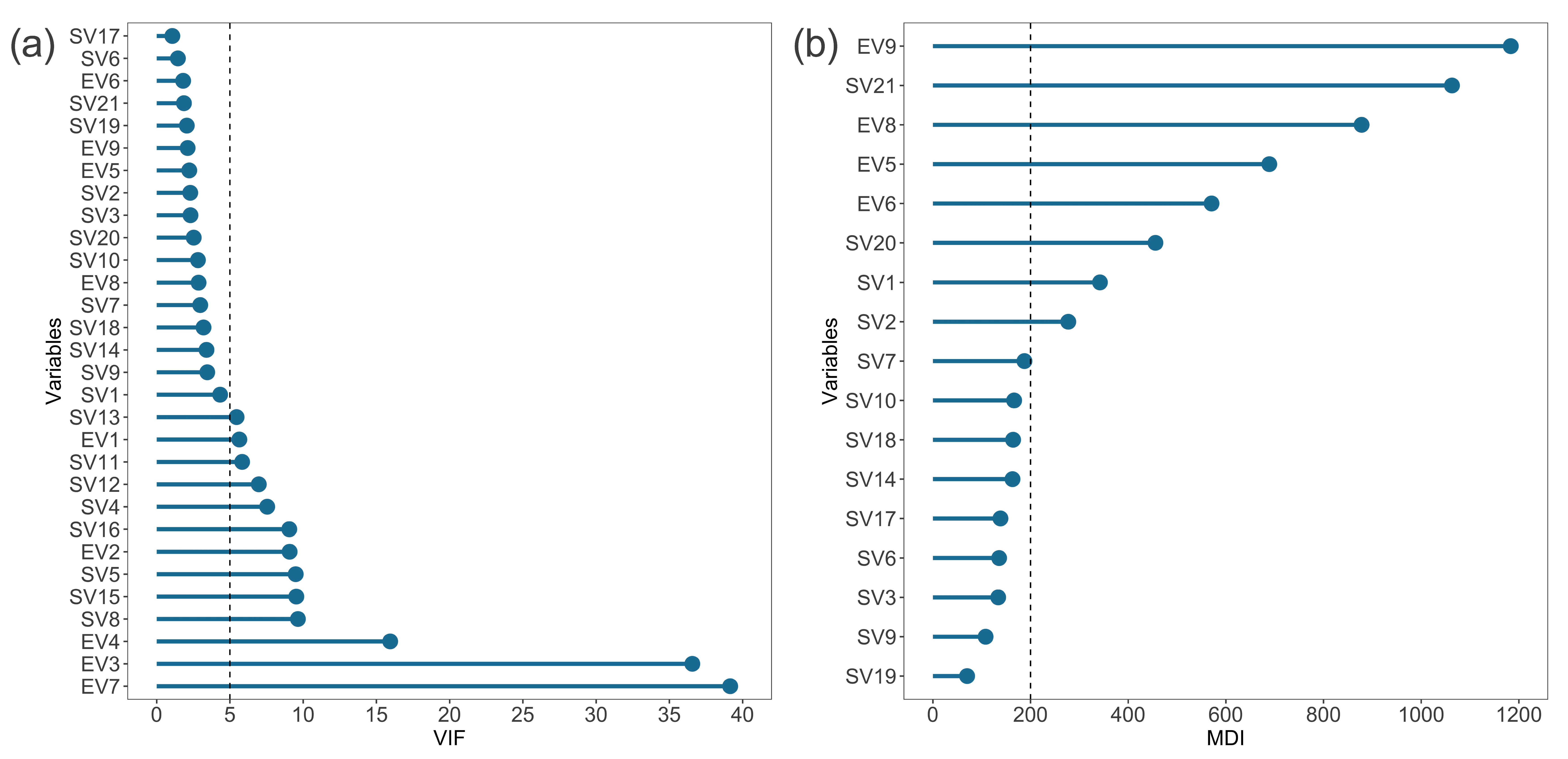
2.2.1. Variable Selection

Two widely adopted approaches, namely multicollinearity assessment and random forest [37], were employed in a progressive manner as a screening step for identifying the most representative influencing factors on the tourism industry from 30 candidate variables. Precisely, the indicator variance inflation factor (VIF) was first adopted to measure the multicollinearity effect, referring to a correlation between explanatory factors [38]. Commonly, VIF < 10, representing mild and negligible multicollinearity, is adopted as the threshold to screen variables [39]. Here, given the adequacy of candidate variables involved in this analysis, a stricter standard was adopted, indicating that a candidate variable with VIF > 5 was removed. Following the VIF step, random forest, an integrated machine learning approach relying on the decision tree, was adopted for further screening the explanatory variables according to the calculation of an indicator named mean decrease impurity (MDI), which has been commonly used for reflecting the ranking of a factor’s relative importance [40]. For a candidate variable, a higher value of MDI is associated with the increased importance of the variable. This random forest step is typically empirical and data-driven, as MDI is not a relative measure [41].

2.2.2. Bayesian STVC Model

The Bayesian spatiotemporally varying coefficients (STVC) model is a recently burgeoning local spatiotemporal regression developed under the Bayesian hierarchical modeling (BHM) framework. It is mainly designed to quantitatively characterize structured and heterogeneous spatiotemporal impacts (expressed as local-scale coefficients) of different covariates on the outcomes of the variable of interest, that is, to explore the spatiotemporal nonstationarity inherent in geospatial research phenomena [35,36].
For China’s tourism case, Y i t denotes the space–time monitoring data of the total tourism revenue indicator, in which i = 1 , , I (I = 343) are the administrative geographical units of the cities. For each city, data are available for a ten-year period from 2008 to 2017, labeled as t = 1 , , T (T = 10). Then, the structured additive predictor ζ i t = g ( Y i t ) within a reduced Bayesian STVC model is formulated in Equations (1)–(3), i.e.,
ζ i t = g ( Y i t ) = η + k = 1 K f s p a c e ( ω i k S X i t k ) + m = 1 M f t i m e ( φ t m T X i t m ) ,
ω i | ω i , τ ω ,   W ~ N ( j = 1 I w i j ω j i = 1 I w i j , 1 τ ω i = 1 I w i j ) , i = 1 , , I ,
φ t + 1 φ t | τ φ ~ N ( 0 , 1 τ φ ) , t = 1 , , T 1 ,   or
φ t 2 φ t + 1 + φ t + 2 | τ φ ~ N ( 0 , 1 τ φ ) , t = 1 , , T 2 ,
In Equation (1), g ( ) denotes a log-Gaussian likelihood function for this case to link Y i t and ζ i t . η denotes the intercept with fixed effect. S X signifies K main covariates with the spatial nonstationary assumption. T X represents M main covariates that are assumed to be temporally nonstationary. The parameter ω i k is named as space-coefficients (SCs) and φ t m is named time-coefficients (TCs), which are two fundamental outputs of the STVC model. f s p a c e ( ) and f t i m e ( ) signify the spatial and temporal latent Gaussian models (LGMs) that are used for fitting the random effects of spatial and temporal nonstationarity to estimate local parameters SCs and TCs [42,43].
In Equation (2), on account of the spatial LGM f s p a c e ( ) , the prior intrinsic conditional autoregressive (iCAR) model is adopted for fitting the spatial autocorrelation characteristics that are also called the spatial structured random effects within a BHM [44], where ω i denotes every spatial unit in ω apart from the i-th spatial unit, W = ( w i j ) represents the spatial relation matrix in which w i j = 1 if spatial units i and j are neighbors, e.g., spatial adjacency relations here, and w i j = 0 otherwise, as well as τ ω further indicates the precision parameter [45].
In Equation (3), the prior random walk (RW) model is used as the temporal LGM f t i m e ( ) to estimate the temporal autocorrelation characteristics of TCs, where the structured temporal random effect of covariates φ can be a random walk of order one or two, with τ φ being the precision parameter [46]. The prior RW model of order two is more suitable for the research object with a clear linear time trend, compared with the prior RW model of order one.

2.2.3. Model Implementation and Comparison

To explore both the global homogeneous and local heterogeneous impacts of socioeconomic and environmental factors on city-specific outcomes of China’s tourism, we implemented four types of Bayesian regressions, the multiple linear regression (MLR, model 1), the ordinary generalized additive model (GAM, model 2), the global spatiotemporal regression (model 3), and the Bayesian STVC model (model 4), which belongs to the local spatiotemporal regression family. We chose these models based on the following considerations. First, model 1 and model 2 were traditional mainstream models. We used them to fit the overall linear and nonlinear impacts of covariates on tourism [47]. Then, we used a widely applied spatiotemporal regression (model 3), which mainly served as a spatiotemporal descriptive tool, to depict the original smoothed spatial variations and temporal trends of tourism in China [42]. However, models 1–3 are regarded as the global-based type of regression, meaning that covariate impacts (coefficients) were homogeneous across space and over time [35]. Given this underlying limitation of stationarity, model 4 was finally employed to explore the structured heterogeneous (varying) impacts of covariates at both space and time scales [36].
To be specific, the equation of an MLR (model 1) is given by
ζ i t = g ( Y i t ) = η + k = 1 K χ k X i t k ,
where χ k denotes the overall coefficient of the k-th covariate X , which qualifies the linear numerical impacts of explanatory factors on Y i t .
An ordinary GAM (model 2) is formulated as [48]
ζ i t = g ( Y i t ) = η + k = 1 K f G A M ( δ h k X i t k ) ,
where f G A M ( ) denotes the nonparametric smooth function for fitting a set of coefficients δ h k with h groups, representing the numerical nonlinear impacts of the k-th covariate. Unlike model 1, model 2 is useful in identifying response–covariate numerical nonlinear relationships. However, both model 1 and model 2 cannot consider the spatiotemporal effects essential for geospatial analysis.
A global spatiotemporal regression (model 3) can be modeled with [42,46,49]
ζ i t = g ( Y i t ) = η + k = 1 K χ k X i t k + f s p a c e ( μ i ) + f t i m e ( λ t ) ,
where μ i signifies the space-intercepts (SIs) representing the structured spatial distribution of Y i t , λ t signifies the time-intercepts (TIs) representing the structured temporal trend of Y i t , LGMs f s p a c e ( ) and f t i m e ( ) are the same as in Equation (1).
Model 4, as fully introduced in Equations (1)–(3), has been as a reduced Bayesian STVC regression by removing the spatiotemporal random effects of intercepts to ensure noticeable variations of both spatial and temporal nonstationary impacts of different explanatory factors on the target response variable [36,50].
Finally, the optimal model from the above four regressions with the best model fitness and predictability was further utilized to estimate the complete spatiotemporal maps of Y i t .

2.2.4. Model Inference and Evaluation

Alternative regression models were established using the Bayesian statistics based on the advanced hierarchical modeling strategy, that is, a BHM framework. Non-informative priors were assigned to parameters within the BHM to embody the idea of data-driven modeling [47]. The integrated nested Laplace approximation (INLA) algorithm, an approximate Bayesian inference technique, was adopted to estimate these regression models using the R-INLA package in the R environment [51] due to its advantage of producing reliable estimated results with a relatively short computation time [52]. The performances of these alternative regressions are evaluated in terms of three aspects, including the degree of model fitting, model complexity, and predictive ability [46]. Specifically, the deviation information criterion (DIC) [53] and the Watanabe–Akaike information criterion (WAIC) are used for reflecting the degree of fitting of the Bayesian regression, for which a smaller value indicates a better model fit. Likewise, the complexity of the Bayesian regression is evaluated with two indices ( P D I C and P W A I C ) that can be simultaneously obtained via the adoption of both the DIC and WAIC methods, for which smaller values are also reflective of better model performances. In terms of the model predictive power, a logarithmic score (LS) retrieved from the conditional predictive ordinates under a leave-one-out cross-validation is used, with smaller values associated with better predictive capacities [54].

3. Results

3.1. Selected Drivers for Modeling

As indicated in Figure 2, through setting VIF < 5 as the inclusion criteria, potential explanatory variables with higher rankings of MDI were selected from the screening outcomes and were added into the regression modeling. To be specific, first, we removed factors with higher multicollinearity based on the exclusion threshold of 5 for VIF, as shown in Figure 2a. This step left 13 socioeconomic factors (i.e., SV1, SV2, SV3, SV6, SV7, SV9, SV10, SV14, SV17, SV18, SV19, SV20, and SV21) and four environmental factors (i.e., EV5, EV6, EV8, and EV9). Further, using Figure 2b, we selected the top eight factors (i.e., EV9, SV21, EV8, EV5, EV6, SV20, SV1, and SV2), which had relative higher importance (contribution) to the response variable. Because the selection of MDI is generally empirical, here, the main reason for our choice of MDI is that there was an apparent bluff trend between the two factors of SV2 and SV7. The top eight factors covered four socioeconomic factors and four environmental factors, which was ideal for exploring the combined impacts of the above two critical aspects on tourism development. Hence, based on the perspectives above, the screening threshold applicable to this case is MDI > 200. Summing up the above, a core variables system particularly applicable to China’s tourism case was created, which contained a total of eight critical factors (renamed as X1–X8 in Table 3), and was further incorporated into the next-step regression analysis.

3.2. Model Assessment and Comparison

We assessed the four types of comparative Bayesian regression models’ performances by jointly considering model fitness, complexity, and predictive power, for which a total of five representative evaluation indicators are summarized in Table 2. Model 4 (STVC) showed the best performance with the minimum assessment indicators DIC, WAIC, and LS. However, for P D I C and P W A I C , model 4 demonstrated a notable deficiency and it presented a much higher complexity than the other three mainstream benchmark models. The complexity ( P D I C ) of model 4 was found to be about 99 times higher than that of a multiple linear regression (model 1), which was 2.6 times higher than that of a global spatiotemporal regression (model 3). Two possible reasons were considered for explaining the increased complexity of the STVC model. Specifically, the STVC model demonstrated both superior model fitness and predictive capacity compared with all the other regressions. Moreover, it should be pointed out that the STVC model was the only one that had the capacity for synchronously detecting both temporal and spatial heterogeneous associations between variables to be further interpreted at a space-time scale. Therefore, model 4 (STVC) was selected as the final regression to explore the spatiotemporal heterogeneous relationships between tourism and eight selected explanatory variables, which was also used for producing a series of estimated spatiotemporal distribution maps reflective of the city-level tourism revenue in China.

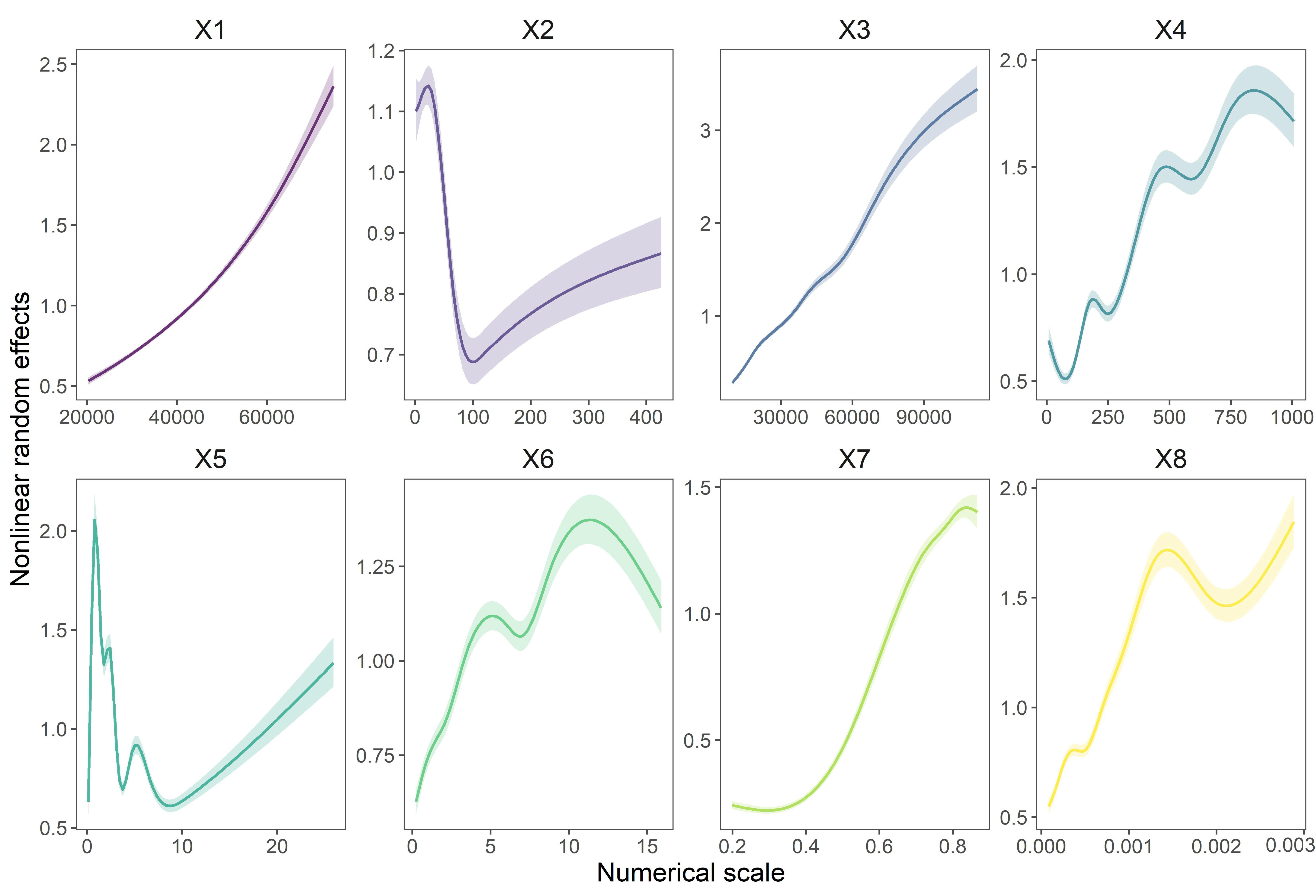
3.3. Global-Scale Impacts of Drivers

Two kinds of overall impacts of socioeconomic and environmental variables on tourism were estimated: one was the global-scale linear numerical effects based on model 1; the other one was the global-scale nonlinear numerical effects obtained from model 2. We summarized the critical parameters of model 1 in Table 3, including the overall coefficients representing the stationary relationship among variables, standard deviation (SD), and the 2.5% and 97.5% quantiles of Bayesian credible intervals (CIs). In terms of the four socioeconomic variables, X1 and X2 reflected the income level of individual residents, X3 represented the regional macroeconomic development conditions, and X4 represented the population condition. For the other four environmental variables, X5 and X7 represented the city-specific urbanization process and vegetation coverage based on satellite remote sensing data, respectively. X6 and X8 reflected the general geographical situations characterized by topography and transportation, respectively. Except for X2 and X5, the overall coefficients of the other six factors were found to be greater than zero. This finding indicated that most core variables served as positive stimulants for tourism development from a global-scale perspective. Notably, the NDVI (X7), the average wage of employees in urban units (X1), GDP per capita (X3), and road network density (X8) demonstrated more significant impacts on tourism among the eight factors.
Furthermore, the exponent-scale nonlinear numerical effects of the eight selected drivers were illustrated in Figure 3. We noticed that all the variables’ numerical influencing curves had a similar upward trend. At the same time, we identified the varying impacts of each variable across their development process. It is worth mentioning that X2 and X5 were negatively linearly correlated with the tourism industry, which could not be explained directly. While by further analyzing the nonlinear results, only X2 and X5 appeared to have a significant downward trend, leading to the overall negative linear association in Table 3. This finding proved that model 2 had a superior interpretation capacity over model 1 in fitting global-scale numerical impacts. However, both linear and nonlinear numerical modeling results were produced based on a stationary assumption. As a result, these global-scale outputs might smooth or hide the local-scale heterogeneous impacts of different variables on the tourism industry over the entire study area and time frame, particularly for a fine-scale space–time dataset.

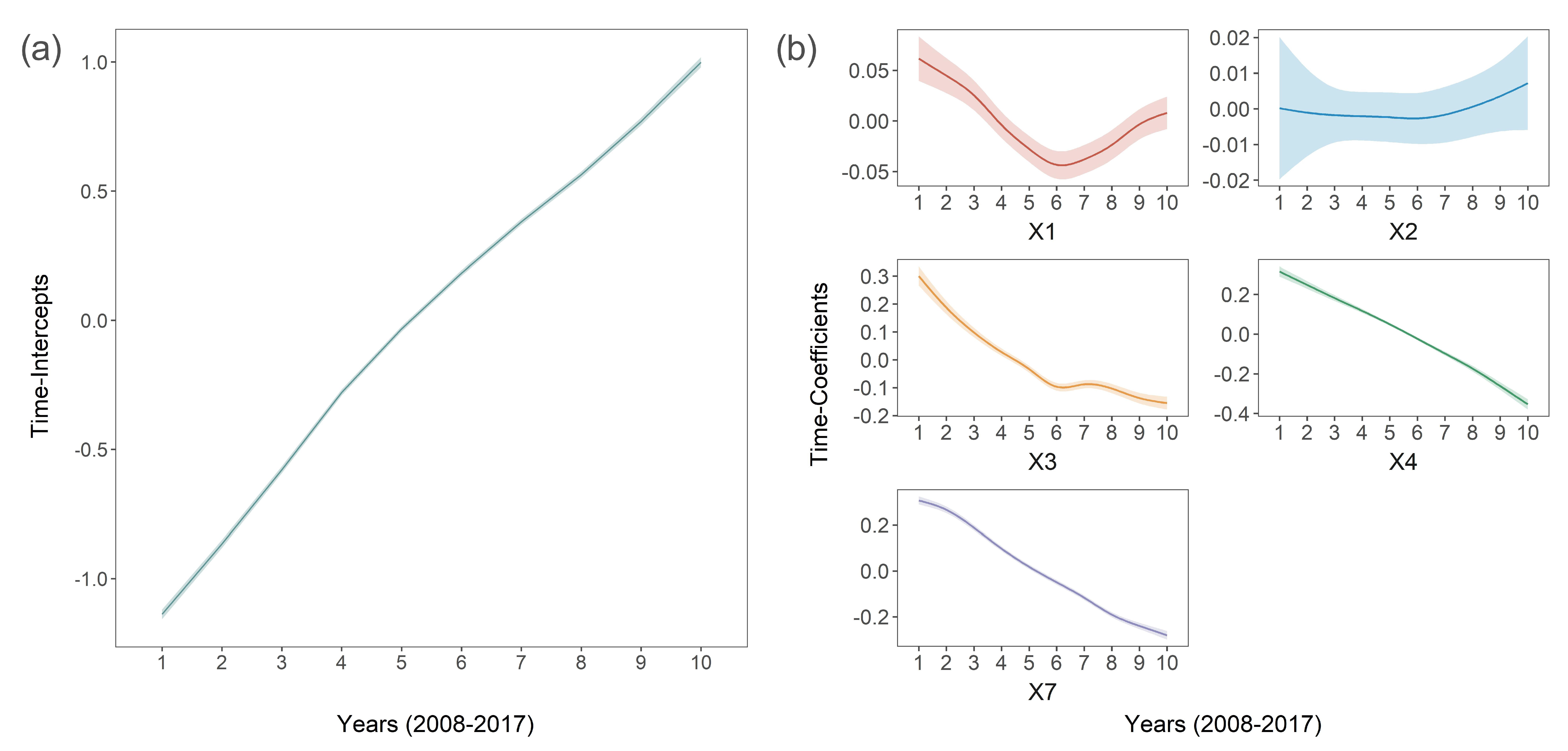
3.4. Temporally Varying Impacts of Drivers

In Figure 4, we presented a TIs graph and five TCs graphs with 95% Bayesian CIs, to exhibit the crude temporal dynamic trend of tourism and the temporally heterogeneous impacts of main drivers on tourism in China, as well as the uncertainties of these estimated parameters. According to Figure 4a, China’s tourism development level demonstrated a continuously increasing trend from 2008 to 2017, meaning that China’s tourism industry maintained a high development speed spanning ten years. Furthermore, it can be seen from Figure 4b that the temporal tourism–covariates relationships varied non-linearly over 2008–2017. This visualization of local-scale nonstationary regression relationships over periods was an essential feature of the Bayesian STVC model that cannot be facilitated via the adoption of global-scaled coefficients. Generally speaking, X3 (GDP per capita), X4 (population density), and X7 (NDVI) showed a downward trend from 2008 to 2017, which indicated a strong to weak impact of these variables on tourism development over time. While X1 (average wage of employed persons in urban units) and X2 (employment density of urban units) presented an initial downtrend, followed by an upward tendency starting from 2013, suggesting that their roles in promoting tourism development gradually especially after 2013. These findings also meant that groups with high quality of living might be a potentially vital force to promote tourism. In addition, we noticed that the TCs of X1 and X2 had relatively higher uncertainties (CIs) due to the fluctuation ranges of TCs of X1 (−0.05–0.05) and X2 (−0.02–0.02) being much narrower compared with those of the other indicators, e.g., X4 (−0.4–0.2). In fact, when we plotted all the factors within a single graph using the same vertical coordinate, the uncertainties (CIs) of X1 and X2 turned out to be very small; however, the time trends of X1 and X2 could be smoothed out. From this perspective, the uncertainties of all indicators were within an acceptable range.

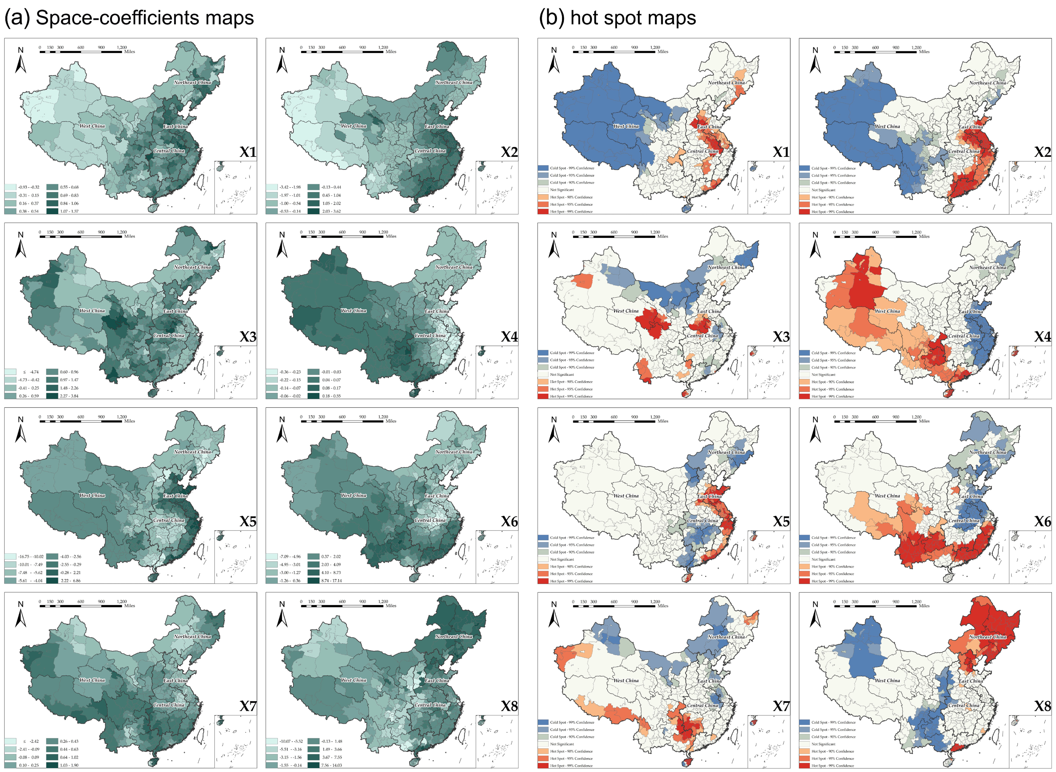
3.5. Spatially Varying Impacts of Drivers

Spatially, we retrieved the parameters of SIs from model 3 to geographically map the ten-year average tourism revenue distribution across China, as presented in Appendix A Figure A1. In addition, utilizing the SCs parameters from model 4, the variables’ spatial nonstationary maps were depicted in Figure 5a. The cluster maps for parameter SCs were also produced to highlight those significant (>90% confidence) hot spots and cold spots at the city level, as shown in Figure 5b.
From Figure A1, the spatial distribution characteristics of China’s tourism revenue demonstrated a gradual increase from West China to East China. Simultaneously, we detected diverse geospatial tourism–covariates relationships at the city level from Figure 5a and an apparent spatial agglomeration effect of SC maps in Figure 5b. In fact, for every single factor of interest, city-specific areas with higher sensitivity to this particular covariate could be visually identified in terms of achieving regional tourism development, based on direct analysis of the corresponding SC map produced by that covariate. Furthermore, within each city area, a series of urban policies could be proposed to facilitate its tourism development based on the relative impacts of the eight-core variables. The relative effect of each covariate within each city could be assessed by vertically integrating the local-scale information from all the SC maps together [50].
Looking at the macroscopic regional scale using the hot spot maps in Figure 5b, we may discover that: in Northeast China, X8 may serve as an essential factor for promoting the development of the local tourism industry, while X5 and X6 may have no impacts, and the other factors may also have an individual city-specific impact yet without generating geographic hotspot regions in the past. Likewise, the high-level tourism development in China’s eastern region may be mainly promoted by X2 and X5; and X4 are not entirely essential. In Western China, with low-level tourism development, X4 may be a primary determinant to improve its tourism conditions. Meanwhile, X6 and X7 also present spatially positive clustered effects in some areas, such as Yunnan and Sichuan. In the regions of Central China, tourism development seems to be dominated by socioeconomic factors, including X1, X2, and X3.

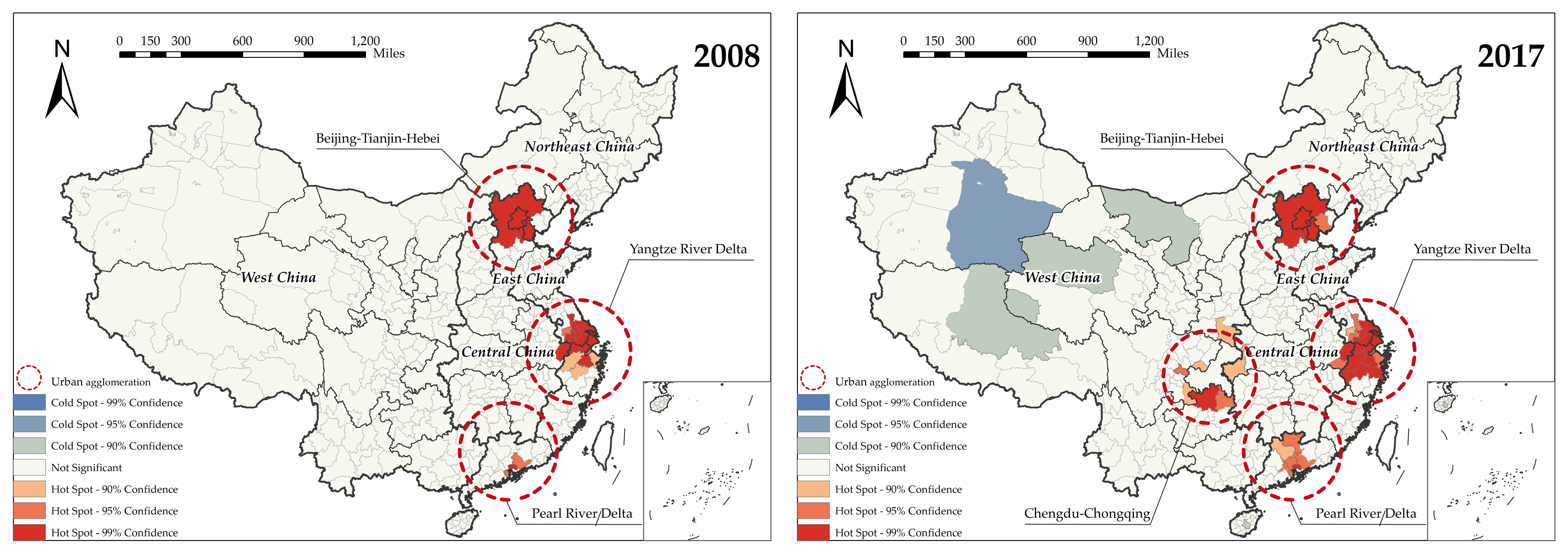
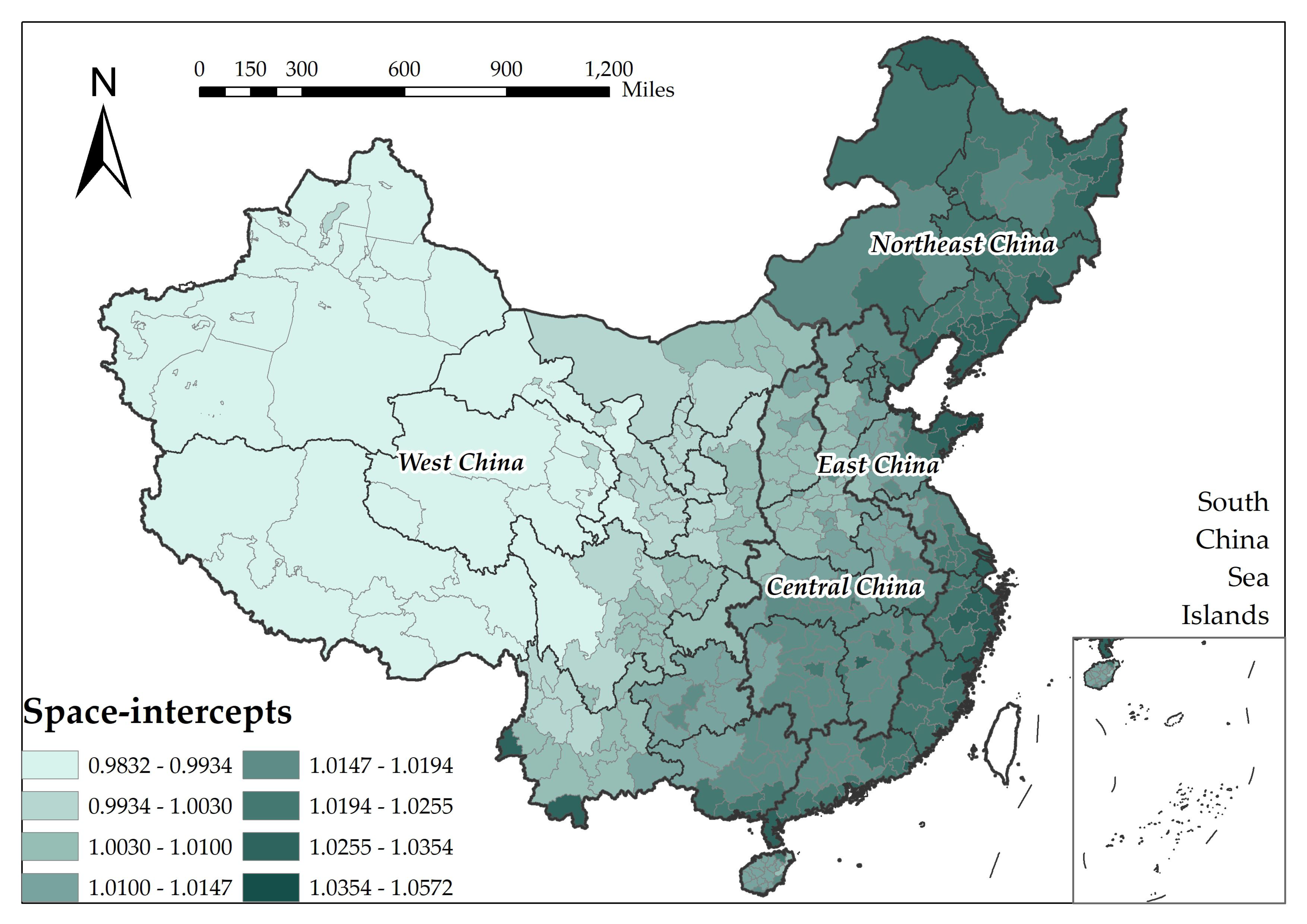
3.6. Spatiotemporal Estimated Maps of China’s City-Level Tourism Revenue

A complete series of spatiotemporal distribution maps of China’s city-specific tourism development level from 2008 to 2017 was produced by adopting the optimal Bayesian STVC model (model 4), as shown in Figure 6. The newly model-estimated tourism maps highlighted hidden areas (e.g., cities with missing values) and provided more intuitive information (e.g., smooth the city-level extreme outliers), which were expected to assist in making policies about the sustainable development of tourism. Generally, the overall growth in the city-level tourism industry was identified over the past decade in China, during which time diverse improvement intensities were found among regions at a local city scale. In Central China, since 2008, about 77% of blue-colored cities with weak tourism industries gradually shifted to yellow/red colors with relatively strong tourism industries. In contrast, such a shifting proportion of East China was about 55%, suggesting that Central China’s tourism industry grew faster than that of eastern cities. In terms of West China and Northeast China, the shifting proportions were about 51% and 41%, respectively, which were relatively lower than the other two divisions. In 2017, the low-tourism-level cities with a blue color were mainly distributed in the provinces of Heilongjiang, Gansu, Ningxia, Xinjiang, Qinghai, and Tibet.
Lastly, we performed a hot spot analysis for the newly estimated complete tourism maps in 2007 and 2018, respectively, to detect those significant city clusters (>90% confidence) of the tourism industry, as shown in Figure 7. In 2017, we found four significant tourism industry clusters (hot spots) and one less-developed tourism region (cold spot) at the city level, compared with 2008 with two clearly formed hot spots of the tourism industry. These four identified high-level tourism city clusters in 2017 were demonstrated to be consistent with China’s top four major urban agglomerations, namely, Beijing–Tianjin–Hebei, the Yangtze River Delta, the Pearl River Delta, and the Sichuan–Chongqing Region. This might reveal that current tourism agglomeration development is closely related to the urbanization degree. Meanwhile, a cold spot was detected in West China, indicating that the tourism development of western cities was relatively slow.

4. Discussion

In this study, the multidimensional impacts of socioeconomic and environmental variables, including linear and nonlinear numerical effects and spatiotemporal heterogeneous effects, on regional tourism were comprehensively investigated across Chinese cities along with the first production of a set of spatiotemporal maps depicting China’s total tourism revenue. These findings may add innovative insights about the mechanisms of how multi-source geospatial factors have affected the regional tourism industry, and is expected to provide a brand-new viewpoint for policymakers. According to different scales, we have some conclusions, as follows.
Globally, significant effects of both socioeconomic and environmental variables were identified [28,55,56,57], which highlighted the necessity of taking a wide range of factors into accounts throughout the procedure of tourism policies formulation. Tourism is a comprehensive industry composed of multiple elements, including food, shelter, transportation, travel, entertainment, and purchase. However, the importance of some of these elements embedded in the tourism industry, such as food, shelter, and transportation, is always ignored for the reason that they are simply regarded as the basic service facilities of a city. Therefore, the positive effects of the socioeconomic and environmental factors on tourism are supposed to be focused on the industrial level, which suggests that the idea of developing industries should always be adopted as the guideline for developing the tourism industry regardless of regional or national levels. At present, the “Travel +” strategy being implemented by the Chinese government is exactly based on this idea [58].
Temporally, the development of China’s tourism has mainly benefited from comprehensive time–scale impacts of multiple factors. Based on temporal nonstationarity, the predominant stimulants for tourism development were demonstrated to have gradually switched from the regional economy, populational size, and tourism resource attractiveness to personal economic status. These results implied that China’s current tourism industry demonstrated a new feature that a transition from sightseeing tourism to leisure and holiday tourism is very much likely to occur. Meanwhile, residents’ affluence has been highlighted as an indispensable contributor to nationwide tourism development [59]. Under such a changing background of the tourism industry in China, it is highly suggested that improving personal income, as well as safeguarding the rights and interests of employees, should be adopted as an essential strategy for facilitating the nationwide tourism industry development, which might be achieved via the implementation of multiple tourism-related policies at governmental levels, such as approving paid-leave policies for employees, encouraging enhanced flexibilities of work schedules to be tailored for vocational leaves, as well as encouraging off-peak vocational arrangements.
Spatially, the development of China’s tourism could be characterized as “strong in the east and weak in the west” [30], which was affected by various factors. Cities of West China were mainly affected by population size and tourism resources, while personal income, employment and urbanization had more contributions to cities in the east region [60]. The city-level spatial nonstationarity found in this study could serve as an acceptable reference in the procedure of making more targeted policies by governments at all levels. For example, the western region may put forward corresponding talent introduction policies while promoting economic development. In addition, the local government can develop sightseeing and holiday tourism through developing natural landscapes. Cities of East China need to focus on optimizing the protection system of workers’ rights and interests and developing characteristic tourism products to provide tourists with high-end, comfortable, and personalized services for stimulating tourism. Northeast China may focus on infrastructure and strengthen the planning and laying of the road networks to enhance regional tourism accessibility. Furthermore, city-level local authorities could utilize local resources rationally and determine the direction of tourism strategies by using the critical drivers’ local spatial influencing maps to support ecotourism, sightseeing tourism, vacation tourism, geological tourism, and urban tourism. In addition, the first series of maps displaying China’s tourism revenue’s spatiotemporal distributions at an administrative city level from 2008 to 2017 was produced, which was further analyzed to provide urbanization-related insights into empirically optimizing the unbalanced development of the tourism industry [61,62].
To sum up, from the multidimensional spatiotemporal heterogeneous perspective, the government should formulate various tourism policies based on region-specific conditions, as well as pursue the development concept of “applying proper measurements in line with local conditions and temporal variations”. At present, tourism industry development in areas with relatively high urbanization levels has demonstrated a change from sightseeing tourism to leisure tourism. As a result, socioeconomic status should be continuously considered as a significant factor throughout tourism-related policy-making procedures in these regions. In contrast, regarding cities with low-level urbanization distributed in West China, environmental factors or sightseeing resources, instead of other factors, should be addressed as predominant issues to be considered throughout the formulation of tourism-related policies [60]. Therefore, making city-specific strategies that take city-specific factors into account is expected to improve the accuracy of policy formulation, as well as the effectiveness of strategic implementation, which would further mitigate both “invalid policy” and “weak policy” produced by the “one-size-fits-all” policy.
Finally, we would like to underline the importance of the local spatiotemporal regression approach, namely, the Bayesian STVC model we have selected. As discussed above, introducing a spatiotemporal heterogeneous perspective to regional tourism management could avoid the one-size-fits-all issue via providing multidimensional spatiotemporal information. In the spatial statistics field, local regressions that can deal with such spatiotemporal heterogeneity among variables relationships (spatiotemporal nonstationarity) are relatively rare, which can be generally classified into the frequentist-type model [63,64,65] and the Bayesian-type model [35,36,66], as they were proposed independently under different statistical traditions. The main reasons we chose the Bayesian STVC model as the applied local spatiotemporal regression lie in the following considerations. First, only the Bayesian-based local spatial or spatiotemporal model is an actual “full-map” modeling technique; thus, the results are more reliable [67,68]. Second, the Bayesian STVC model follows a space–time independent nonstationary assumption, dramatically reducing the computational burden and weakening the overfitting problem. Last but not least, due to its separately fitting of space-coefficients (SCs) and time-coefficients (TCs), the Bayesian STVC model is more user-friendly: stakeholders can directly separately obtain the spatial and temporal autocorrelated regularities [36,50]. Beyond these benefits, the Bayesian STVC model still needs further improvement to solve more complex space–time interaction issues in natural and social sciences.

5. Conclusions

This study verifies that socioeconomic and environmental factors simultaneously affect tourism development over China, globally and locally, supported by the up-to-date space-time data of city-level tourism statistics and a series of advanced Bayesian regressions. Remarkably, the local impacts of socioeconomic and environmental conditions vary heterogeneously at the city level in both time and space dimensions across China, and was demonstrated by adopting the cutting-edge Bayesian STVC model, which was also used for estimating the first series of spatiotemporal maps of city-level tourism development. These fruitful findings provide novel insights into policy-making procedures at multiple levels. Here, the Bayesian STVC model was successfully applied to mine the spatial and temporal autocorrelated nonstationarity inherent in tourism–covariates relationships over China and could serve as an emerging tool to offer new insights on spatiotemporal-oriented influencing factor analysis and high-precision prediction in broader GIScience-related fields of social and natural sciences.
Apart from all these achievements, several concerns should be better addressed in future lines of research. First, the seasonal effect is the main factor affecting tourists’ behavior [69], which emphasizes collecting and using quarterly tourism data in tourism research. However, this study is limited because national urban tourism data sources only have annual scale records. Second, other underlying tourism-related factors such as tourism resources were not fully considered in this study [34]. Future studies might focus on a relatively small area with seasonal heterogeneity by using multi-source tourism data to construct more scientific indicators [70] and developing more sophisticated spatiotemporal statistical models for outputting more informative results for regional tourism research.

Author Contributions

Conceptualization, Chengwu Wang and Chao Song; data curation, Xu Zhang, Zhangying Tang and Honghu Tang; formal analysis, Xu Zhang, Chao Song, and Chengwu Wang; funding acquisition, Chao Song, Chengwu Wang and Zhangying Tang; investigation, Chengwu Wang and Xu Zhang; methodology, Chao Song and Zhoupeng Ren; project administration, Chao Song; software, Chao Song and Mingyu Xie; visualization, Xu Zhang, Chao Song, Mingyu Xie and Honghu Tang; writing—original draft, Xu Zhang; writing—review and editing, Chao Song, Chengwu Wang and Yili Yang. All authors have read and agreed to the published version of the manuscript.

Funding

This work was collaboratively supported by the National Natural Science Foundation of China (Grant No. 42071379 and 41701448), the State Key Laboratory of Resources and Environmental Information System (Grant No. 201811), the Applied Basic Research Funded Project of Sichuan Science and Technology Department (Grant No. 2020YJ0117), the Humanities and Social Sciences Research Fund Project of Southwest Petroleum University (Grant No. 2019RW021), the Chengdu Federation of Social Science Association (Grant No. 2021ZC003), and the Fund for Introducing Talents of Sichuan University (Grant No. YJ202157). The funders had no conflicts in study design, data collection and analysis, decision to publish, or manuscript preparation.

Data Availability Statement

Publicly available datasets were analyzed in this study. The tourism and socioeconomic data can be found in China City Statistical Yearbook and Statistical Bulletin. The environmental data can be found here: http://data.cma.cn/ (accessed on 28 April 2021) and http://www.resdc.cn/ (accessed on 28 April 2021).

Conflicts of Interest

The authors declare no conflict of interest.

Appendix A

Figure A1. Space-Intercepts (SIs) map: the model-estimated geographical variations of China’s ten-year average total tourism revenue at the city level during 2008–2017.
Ijgi 10 00410 g0a1

References

  1. Fayissa, B.; Nsiah, C.; Tadasse, B. Impact of tourism on economic growth and development in Africa. Tour. Econ. 2008, 14, 807–818. [Google Scholar] [CrossRef] [Green Version]
  2. Travel & Tourism Global Economic Impact & Issues 2017. Available online: https://wttc.org/Portals/0/Documents/Reports/2020/Global%20Economic%20Impact%20Trends%202020.pdf?ver=2021-02-25-183118-360 (accessed on 6 June 2021).
  3. Modeste, N.C. The impact of growth in the tourism sector on economic development: The experience of selected Caribbean countries. Econ. Internazionale/Int. Econ. 1995, 48, 375–385. [Google Scholar]
  4. Proença, S.; Soukiazis, E. Tourism as an economic growth factor: A case study for Southern European countries. Tour. Econ. 2008, 14, 791–806. [Google Scholar] [CrossRef]
  5. Ma, T.; Hong, T.; Zhang, H. Tourism spatial spillover effects and urban economic growth. J. Bus. Res. 2015, 68, 74–80. [Google Scholar] [CrossRef]
  6. Coccossis, H. Tourism and sustainability: Perspectives and implications. In Sustainable Tourism? European Experiences; CAB INTERNATIONAL: Wallingford, UK, 1996; pp. 1–21. [Google Scholar]
  7. Joshi, O.; Poudyal, N.C.; Larson, L.R. The influence of sociopolitical, natural, and cultural factors on international tourism growth: A cross-country panel analysis. Environ. Dev. Sustain. 2017, 19, 825–838. [Google Scholar] [CrossRef]
  8. Khan, A.; Bibi, S.; Ardito, L.; Lyu, J.; Hayat, H.; Arif, A.M. Revisiting the Dynamics of Tourism, Economic Growth, and Environmental Pollutants in the Emerging Economies—Sustainable Tourism Policy Implications. Sustainability 2020, 12, 2533. [Google Scholar] [CrossRef] [Green Version]
  9. Tuckova, Z.; Sverak, P. Impact of the Regional Macroeconomics Indicators on Tourism Entities in Plzen and Zlin Regions. Procedia Econ. Financ. 2016, 39, 313–318. [Google Scholar] [CrossRef] [Green Version]
  10. Jarvis, D.; Stoeckl, N.; Liu, H.-B. The impact of economic, social and environmental factors on trip satisfaction and the likelihood of visitors returning. Tour. Manag. 2016, 52, 1–18. [Google Scholar] [CrossRef] [Green Version]
  11. Jayaraman, K.; Lin, S.K.; Haron, H.; Ong, W.L. Macroeconomic factors influencing Malaysian tourism revenue, 2002–2008. Tour. Econ. 2011, 17, 1347–1363. [Google Scholar] [CrossRef]
  12. Alonso-Almeida, M.d.M.; Borrajo-Millán, F.; Yi, L. Are social media data pushing overtourism? The case of Barcelona and Chinese tourists. Sustainability 2019, 11, 3356. [Google Scholar] [CrossRef] [Green Version]
  13. Field, C.B.; Barros, V.R. Climate Change 2014-Impacts, Adaptation and Vulnerability: Part A: Global and Sectoral Aspects: Volume 1, Global and Sectoral Aspects: Working Group II Contribution to the IPCC Fifth Assessment Report; Cambridge University Press: Cambridge, UK, 2014. [Google Scholar]
  14. Hewer, M.J.; Gough, W.A. Thirty years of assessing the impacts of climate change on outdoor recreation and tourism in Canada. Tour. Manag. Perspect. 2018, 26, 179–192. [Google Scholar] [CrossRef]
  15. Martín, M.B.G. Weather, climate and tourism a geographical perspective. Ann. Tour. Res. 2005, 32, 571–591. [Google Scholar] [CrossRef]
  16. Day, J.; Chin, N.; Sydnor, S.; Cherkauer, K. Weather, climate, and tourism performance: A quantitative analysis. Tour. Manag. Perspect. 2013, 5, 51–56. [Google Scholar] [CrossRef]
  17. Smith, T.; Fitchett, J.M. Drought challenges for nature tourism in the Sabi Sands Game Reserve in the eastern region of South Africa. Afr. J. Range Forage Sci. 2020, 37, 107–117. [Google Scholar] [CrossRef]
  18. Atzori, R.; Fyall, A.; Miller, G. Tourist responses to climate change: Potential impacts and adaptation in Florida’s coastal destinations. Tour. Manag. 2018, 69, 12–22. [Google Scholar] [CrossRef]
  19. Susanto, J.; Zheng, X.; Liu, Y.; Wang, C. The impacts of climate variables and climate-related extreme events on island country’s tourism: Evidence from Indonesia. J. Clean. Prod. 2020, 276, 124204. [Google Scholar] [CrossRef]
  20. Kanwal, S.; Rasheed, M.I.; Pitafi, A.H.; Pitafi, A.; Ren, M. Road and transport infrastructure development and community support for tourism: The role of perceived benefits, and community satisfaction. Tour. Manag. 2020, 77, 104014. [Google Scholar] [CrossRef]
  21. Li, L.S.; Yang, F.X.; Cui, C. High-speed rail and tourism in China: An urban agglomeration perspective. Int. J. Tour. Res. 2019, 21, 45–60. [Google Scholar] [CrossRef] [Green Version]
  22. Barkauskas, V.; Barkauskienė, K.; Jasinskas, E. Analysis of macro environmental factors influencing the development of rural tourism: Lithuanian case. Procedia Soc. Behav. Sci. 2015, 213, 167–172. [Google Scholar] [CrossRef] [Green Version]
  23. Marrocu, E.; Paci, R.; Zara, A. Micro-economic determinants of tourist expenditure: A quantile regression approach. Tour. Manag. 2015, 50, 13–30. [Google Scholar] [CrossRef]
  24. Li, M.; Fang, L.; Huang, X.; Goh, C. A spatial–temporal analysis of hotels in urban tourism destination. Int. J. Hosp. Manag. 2015, 45, 34–43. [Google Scholar] [CrossRef] [PubMed]
  25. Gutiérrez, J.; García-Palomares, J.C.; Romanillos, G.; Salas-Olmedo, M.H. The eruption of Airbnb in tourist cities: Comparing spatial patterns of hotels and peer-to-peer accommodation in Barcelona. Tour. Manag. 2017, 62, 278–291. [Google Scholar] [CrossRef] [Green Version]
  26. Xu, D.; Huang, Z.; Hou, G.; Zhang, C. The spatial spillover effects of haze pollution on inbound tourism: Evidence from mid-eastern China. Tour. Geogr. 2020, 22, 83–104. [Google Scholar] [CrossRef]
  27. Brunsdon, C.; Fotheringham, S.; Charlton, M. Geographically weighted regression. J. R. Stat. Soc. Ser. D 1998, 47, 431–443. [Google Scholar] [CrossRef]
  28. Yang, Y.; Fik, T. Spatial effects in regional tourism growth. Ann. Tour. Res. 2014, 46, 144–162. [Google Scholar] [CrossRef] [Green Version]
  29. Shabrina, Z.; Buyuklieva, B.; Ng, M.K.M. Short-Term Rental Platform in the Urban Tourism Context: A Geographically Weighted Regression (GWR) and a Multiscale GWR (MGWR) Approaches. Geogr. Anal. 2020. [Google Scholar] [CrossRef]
  30. Lu, L.; Yu, F. A study on the spatial characteristic of provincial difference of tourism economy. Econ. Geogr. 2005, 3, 406–410. [Google Scholar]
  31. Li, H.; Chen, J.L.; Li, G.; Goh, C. Tourism and regional income inequality: Evidence from China. Ann. Tour. Res. 2016, 58, 81–99. [Google Scholar] [CrossRef]
  32. Yang, Y. Agglomeration density and tourism development in China: An empirical research based on dynamic panel data model. Tour. Manag. 2012, 33, 1347–1359. [Google Scholar] [CrossRef]
  33. Gan, C.; Voda, M.; Wang, K.; Chen, L.; Ye, J. Spatial network structure of the tourism economy in urban agglomeration: A social network analysis. J. Hosp. Tour. Manag. 2021, 47, 124–133. [Google Scholar] [CrossRef]
  34. Wang, D.; Ap, J. Factors affecting tourism policy implementation: A conceptual framework and a case study in China. Tour. Manag. 2013, 36, 221–233. [Google Scholar] [CrossRef]
  35. Song, C.; Shi, X.; Bo, Y.; Wang, J.; Wang, Y.; Huang, D. Exploring spatiotemporal nonstationary effects of climate factors on hand, foot, and mouth disease using Bayesian Spatiotemporally Varying Coefficients (STVC) model in Sichuan, China. Sci. Total Environ. 2019, 648, 550–560. [Google Scholar] [CrossRef] [PubMed]
  36. Song, C.; Shi, X.; Wang, J. Spatiotemporally Varying Coefficients (STVC) model: A Bayesian local regression to detect spatial and temporal nonstationarity in variables relationships. Ann. GIS 2020, 1–15. [Google Scholar] [CrossRef]
  37. Liaw, A.; Wiener, M. Classification and regression by randomForest. R News 2002, 2, 18–22. [Google Scholar]
  38. Vatcheva, K.P.; Lee, M.; McCormick, J.B.; Rahbar, M.H. Multicollinearity in regression analyses conducted in epidemiologic studies. Epidemiology 2016, 6, 227. [Google Scholar] [CrossRef] [PubMed] [Green Version]
  39. Song, C.; He, Y.; Bo, Y.; Wang, J.; Ren, Z.; Guo, J.; Yang, H. Disease relative risk downscaling model to localize spatial epidemiologic indicators for mapping hand, foot, and mouth disease over China. Stoch. Environ. Res. Risk Assess. 2019, 33, 1815–1833. [Google Scholar] [CrossRef]
  40. Breiman, L. Random forests. Mach. Learn. 2001, 45, 5–32. [Google Scholar] [CrossRef] [Green Version]
  41. Genuer, R.; Poggi, J.-M.; Tuleau-Malot, C. Variable selection using random forests. Pattern Recognit. Lett. 2010, 31, 2225–2236. [Google Scholar] [CrossRef] [Green Version]
  42. Blangiardo, M.; Cameletti, M. Spatial and Spatio-Temporal Bayesian Models with R-INLA; John Wiley & Sons: Hoboken, NJ, USA, 2015. [Google Scholar]
  43. Martínez-Bello, D.A.; López-Quílez, A.; Torres Prieto, A. Spatio-temporal modeling of Zika and dengue infections within Colombia. Int. J. Environ. Res. Public Health 2018, 15, 1376. [Google Scholar] [CrossRef] [Green Version]
  44. Lindgren, F.; Rue, H. Bayesian spatial modelling with R-INLA. J. Stat. Softw. 2015, 63, 1–25. [Google Scholar] [CrossRef] [Green Version]
  45. Besag, J. Spatial interaction and the statistical analysis of lattice systems. J. R. Stat. Soc. Ser. B 1974, 36, 192–225. [Google Scholar] [CrossRef]
  46. Blangiardo, M.; Cameletti, M.; Baio, G.; Rue, H. Spatial and spatio-temporal models with R-INLA. Spat. Spatio Temporal Epidemiol. 2013, 4, 33–49. [Google Scholar] [CrossRef] [Green Version]
  47. Wang, X.; Yue, Y.; Faraway, J.J. Bayesian Regression Modeling with INLA; Chapman and Hall/CRC: London, UK, 2018. [Google Scholar]
  48. Hastie, T.J.; Tibshirani, R.J. Generalized Additive Models; CRC Press: Boca Raton, FL, USA, 1990; Volume 43. [Google Scholar]
  49. Ugarte, M.D.; Adin, A.; Goicoa, T.; Militino, A.F. On fitting spatio-temporal disease mapping models using approximate Bayesian inference. Stat. Methods Med Res. 2014, 23, 507–530. [Google Scholar] [CrossRef]
  50. Song, C.; Wang, Y.; Yang, X.; Yang, Y.; Tang, Z.; Wang, X.; Pan, J. Spatial and Temporal Impacts of Socioeconomic and Environmental Factors on Healthcare Resources: A County-Level Bayesian Local Spatiotemporal Regression Modeling Study of Hospital Beds in Southwest China. Int. J. Environ. Res. Public Health 2020, 17, 5890. [Google Scholar] [CrossRef]
  51. Rue, H.; Martino, S.; Chopin, N. Approximate Bayesian inference for latent Gaussian models by using integrated nested Laplace approximations. J. R. Stat. Soc. Ser. B 2009, 71, 319–392. [Google Scholar] [CrossRef]
  52. Rue, H.; Riebler, A.; Sørbye, S.H.; Illian, J.B.; Simpson, D.P.; Lindgren, F.K. Bayesian computing with INLA: A review. Annu. Rev. Stat. Its Appl. 2017, 4, 395–421. [Google Scholar] [CrossRef] [Green Version]
  53. Spiegelhalter, D.J.; Best, N.G.; Carlin, B.P.; Van Der Linde, A. Bayesian measures of model complexity and fit. J. R. Stat. Soc. Ser. B 2002, 64, 583–639. [Google Scholar] [CrossRef] [Green Version]
  54. Held, L.; Schrödle, B.; Rue, H. Posterior and cross-validatory predictive checks: A comparison of MCMC and INLA. In Statistical Modelling and Regression Structures; Springer: Cham, Switzerland, 2010; pp. 91–110. [Google Scholar]
  55. Wang, J.; Huang, X.; Gong, Z.; Cao, K. Dynamic assessment of tourism carrying capacity and its impacts on tourism economic growth in urban tourism destinations in China. J. Destin. Mark. Manag. 2020, 15, 100383. [Google Scholar] [CrossRef]
  56. Gu, M.; Wong, P.P. Residents’ perception of tourism impacts: A case study of homestay operators in Dachangshan Dao, North-East China. Tour. Geogr. 2006, 8, 253–273. [Google Scholar] [CrossRef]
  57. Yin, P.; Lin, Z.; Prideaux, B. The impact of high-speed railway on tourism spatial structures between two adjoining metropolitan cities in China: Beijing and Tianjin. J. Transp. Geogr. 2019, 80, 102495. [Google Scholar] [CrossRef]
  58. Li, J. Research on the Development of Coastal Rural Tourism in China from the Perspective of Industrial Integration. J. Coast. Res. 2020, 115, 271–273. [Google Scholar] [CrossRef]
  59. Lin, V.S.; Qin, Y.; Li, G.; Wu, J. Determinants of Chinese households’ tourism consumption: Evidence from China Family Panel Studies. Int. J. Tour. Res. 2020. [Google Scholar] [CrossRef]
  60. Pratt, S. Potential economic contribution of regional tourism development in China: A comparative analysis. Int. J. Tour. Res. 2015, 17, 303–312. [Google Scholar] [CrossRef]
  61. Fang, L. Empirical Research on the Impact of Urbanization on Regional Tourism Economy in China Basing on Panel Data. In Proceedings of the 2018 9th International Conference on E-Business, Management and Economics, Waterloo, ON, Canada, 2–4 August 2018; pp. 101–105. [Google Scholar]
  62. Luo, J.M.; Qiu, H.; Goh, C.; Wang, D. An analysis of tourism development in China from urbanization perspective. J. Qual. Assur. Hosp. Tour. 2016, 17, 24–44. [Google Scholar] [CrossRef]
  63. Fotheringham, A.S.; Crespo, R.; Yao, J. Geographical and temporal weighted regression (GTWR). Geogr. Anal. 2015, 47, 431–452. [Google Scholar] [CrossRef] [Green Version]
  64. Huang, B.; Wu, B.; Barry, M. Geographically and temporally weighted regression for modeling spatio-temporal variation in house prices. Int. J. Geogr. Inf. Sci. 2010, 24, 383–401. [Google Scholar] [CrossRef]
  65. Wu, C.; Ren, F.; Hu, W.; Du, Q. Multiscale geographically and temporally weighted regression: Exploring the spatiotemporal determinants of housing prices. Int. J. Geogr. Inf. Sci. 2019, 33, 489–511. [Google Scholar] [CrossRef]
  66. Jiang, H.; Hu, H.; Li, B.; Zhang, Z.; Wang, S.; Lin, T. Understanding the non-stationary relationships between corn yields and meteorology via a spatiotemporally varying coefficient model. Agric. For. Meteorol. 2021, 301, 108340. [Google Scholar] [CrossRef]
  67. Wolf, L.J.; Oshan, T.M.; Fotheringham, A.S. Single and multiscale models of process spatial heterogeneity. Geogr. Anal. 2018, 50, 223–246. [Google Scholar] [CrossRef] [Green Version]
  68. Finley, A.O. Comparing spatially-varying coefficients models for analysis of ecological data with non-stationary and anisotropic residual dependence. Methods Ecol. Evol. 2011, 2, 143–154. [Google Scholar] [CrossRef]
  69. E Silva, F.B.; Herrera, M.A.M.; Rosina, K.; Barranco, R.R.; Freire, S.; Schiavina, M. Analysing spatiotemporal patterns of tourism in Europe at high-resolution with conventional and big data sources. Tour. Manag. 2018, 68, 101–115. [Google Scholar] [CrossRef]
  70. Duca, A.L.; Marchetti, A. Open data for tourism: The case of Tourpedia. J. Hosp. Tour. Technol. 2019, 10, 351–368. [Google Scholar]
Figure 1. Geographical distribution of the original city-level total tourism revenue across China in 2017.
Ijgi 10 00410 g001
Figure 2. Two-step variables screening procedure: (a) remove variables with higher multicollinearity (VIF > 5); (b) select variables with the higher relative importance (MDI > 200).
Ijgi 10 00410 g002
Figure 3. Global-scale nonlinear numerical effects of main drivers on China’s city-level tourism industry: X1—average wage of employed persons in urban units, X2—employment density of urban units, X3—GDP per capita, X4—population density, X5—nighttime light index, X6—slope, X7—NDVI, and X8—road network density.
Ijgi 10 00410 g003
Figure 4. (a) Time-intercepts (TIs) graph: the temporal trend of China’s tourism industry from 2008 to 2017, and (b) time-coefficients (TCs) graphs (covariates’ temporal nonstationarity): the impacts of drivers (X1–X4 and X7) on tourism are varying over ten years. Covariates with time-scale variations: X1—average wage of employed persons in urban units, X2—employment density of urban units, X3—GDP per capita, X4—population density, and X7—NDVI. Shadow areas in each facet are the 95% Bayesian CIs to describe the uncertainties of time-scale parameters.
Ijgi 10 00410 g004
Figure 5. (a) Space-coefficients (SCs) maps (covariates’ spatial nonstationarity): spatially varying impacts of main drivers (X1–X8) on total tourism revenue at city level across China, and (b) hot spot analysis for SCs maps: X1—average wage of employed persons in urban units, X2—employment density of urban units, X3—GDP per capita, X4—population density, X5—nighttime light index, X6—slope, X7—NDVI, and X8—road network density.
Ijgi 10 00410 g005
Figure 6. Estimated spatiotemporal maps for showing dynamic variations of city-level tourism development across China from 2008 to 2017.
Ijgi 10 00410 g006
Figure 7. The urban agglomeration of the tourism industry across Chinese cities in 2008 and 2017: hot spot mapping for the areas’ total tourism revenue, estimated by the optimal Bayesian STVC model.
Ijgi 10 00410 g007
Table 1. City-level potential explanatory variables of regional tourism in China: SV1-21 denote twenty-one socioeconomic factors, and EV1-9 denote nine environmental factors.
IdentifierSocioeconomic VariablesIdentifierEnvironmental Variables
SV1Gross domestic product (GDP) per capita (yuan)EV1Precipitation (0.1 mm)
SV2Population density (person/km2)EV2Temperature (centigrade)
SV3Employment density of the first industry (person/km2)EV3Air pressure (1 N/m2)
SV4Employment density of the Second industry (person/km2)EV4Humidity (hPa)
SV5Employment density of the tertiary industry (person/km2)EV5NDVI (/)
SV6Mobile phone penetration rate (subscriber/person)EV6Road network density (km/km2)
SV7Internet broadband penetration rate (subscriber/person)EV7Elevation (meter)
SV8Local general budget revenue per capita (yuan)EV8Slope (°)
SV9Local government budgetary expenditures per capita (yuan)EV9Nighttime light index (/)
SV10Employees population density (person/km2)
SV11Savings deposits of per capita residents (yuan)
SV12Loans of financial institutions per capita (yuan)
SV13Industrial enterprises density (number/km2)
SV14Social fixed asset investment per capita (yuan)
SV15Social consumable total retail sales per capita (yuan)
SV16Student’s density of ordinary middle school (person/km2)
SV17Student’s density of primary school (person/km2)
SV18Hospital density (number/km2)
SV19Hospital beds per capita (number/person)
SV20Employment density of urban units (person/km2)
SV21Average wage of employed persons in urban units (yuan)
Table 2. Bayesian modeling evaluations of the alternative regressions for China’s tourism case account for model fitness, complexity, and predictive power.
IndexDIC P D I C LSWAIC P W A I C
Model 140,238.399.025.9740,262.8330.05
Model 239,153.7264.895.8139,157.0166.83
Model 331,825.74348.954.7231,848.15338.66
Model 430,307.19899.214.5230,345.55761.76
Model 1–4: multiple linear regression, generalized additive model, global spatiotemporal regression, and local spatiotemporal regression STVC model; DIC: deviance information criterion; WAIC: Watanabe–Akaike information criterion; P D I C : effective number of parameters from DIC; P W A I C : effective number of parameters from WAIC; LS: logarithmic score.
Table 3. Linear numerical impacts of main drivers on China’s city-level tourism industry.
VariablesSocioeconomic and Environmental AspectsMeanSDQ 0.025Q 0.975
X1Average wage of employed persons in urban units0.46940.02120.42780.5110
X2Employment density of urban units−0.14280.0170−0.1761−0.1095
X3GDP per capita0.46600.02580.41540.5165
X4Population density0.21360.02820.15820.2689
X5Nighttime light index−0.01410.0310−0.07500.0467
X6Slope0.10130.02020.06150.1410
X7Normalized Difference Vegetation Index (NDVI)0.66300.01870.62630.6996
X8Road network density0.33820.02260.29370.3826
Publisher’s Note: MDPI stays neutral with regard to jurisdictional claims in published maps and institutional affiliations.

