Towards Measuring Shape Similarity of Polygons Based on Multiscale Features and Grid Context Descriptors

Abstract

In spatial analysis applications, measuring the shape similarity of polygons is crucial for polygonal object retrieval and shape clustering. As a complex cognition process, measuring shape similarity should involve finding the difference between polygons, as objects in observation, in terms of visual perception and the differences of the regions, boundaries, and structures formed by the polygons from a mathematical point of view. In existing approaches, the shape similarity of polygons is calculated by only comparing their mathematical characteristics while not taking human perception into consideration. Aiming to solve this problem, we use the features of context and texture of polygons, since they are basic visual perception elements, to fit the cognition purpose. In this paper, we propose a contour diffusion method for the similarity measurement of polygons. By converting a polygon into a grid representation, the contour feature is represented as a multiscale statistic feature, and the region feature is transformed into condensed grid of context features. Instead of treating shape similarity as a distance between two representations of polygons, the proposed method observes similarity as a correlation between textures extracted by shape features. The experiments show that the accuracy of the proposed method is superior to that of the turning function and Fourier descriptor.

1. Introduction

As a metric for distinguishing polygonal geometric features, shape similarity measurement is widely used to match, retrieve, and classify polygons [1]. Scholars have made efforts to retrieve similar polygons to explore building distribution patterns [2] and match corresponding entities [3] for enriching geo-data and mining spatial information hidden in vector datasets. Therefore, calculating a reliable shape similarity measurement result which is consistent with human judgment is a basic stage for completely and accurately unravelling valuable spatial information. For the map generalization task, the completeness and accuracy of its results relies on whether the similar shape judgement is consistent with visual perception [4]. Measuring shape similarity is a complex cognition process relying on two aspects. On the one hand, we can qualitatively determine the difference of polygons as objects in observation regarding visual perception. On the other hand, the difference of the regions, boundaries, and structures formed by the polygons can be quantitatively identified from the mathematical point of view. In existing approaches, polygons are mathematically represented by a series of coefficients or indicators that are invariant to translation, rotation, and scale to derive a similarity measurement for comparing the polygons.

Because shape features are generally derived from the contours of a polygon or the spatial relationships of polygonal regions, the feature representation and description methods can be categorized into contour-based methods, deep learning-based methods and region-based methods [5,6]. Both methods have strengths and weaknesses. Contour-based methods transform a series of vertices of the original shape into a numeric representation, which retains partial geometric features of the shape, uses contours (i.e., polygon boundaries) to describe the shape, and measures the shape similarity by detecting the differences of local contour details [7]. Popular algorithms of this type include the chain code method [8], turning function [9], farthest point method [10], reverse sketch method [11], skeleton line method [12], position graph method [1], and hierarchical model [3]. Because contour-based methods emphasize the interrelationships between vertices, they have the advantage of being computationally efficient. However, the local noise of a contour will influence the topological structure of the resultant shape representation.

The deep-learning based method is essentially representation learning with multiple levels of representations. It learns a way to transform unstructured input into an ideal output representation [13]. Yan et al. proposed a graph convolutional autoencoder (GCAE) model comprising graph convolution and autoencoder architecture to analyze the modeled graph and realize shape coding through unsupervised learning [6]. Although the deep-learning method can identify local and global characteristics in a cognitively compliant manner, it concentrates on polygons without holes.

Region-based methods generate a numeric descriptor in vector form to characterize shape and reflect the internal content of a polygon. Typical methods include geometrical property descriptors, Zernike moments [14], grid-based descriptors [15], shape context [16], and Hu invariant moments [17,18,19]. The representation of shapes in region-based methods focuses on statistically significant features reflecting global information of the shape and morphological characteristics of the internal holes of spatial objects. However, a heavy reliance on region information will inevitably cause the loss of contour details. Since the above-mentioned studies usually only focus on one type of geometric feature that is built on the perspective of mathematical representation, it is hard to capture a complete shape feature from the view of visual perception. Existing methods still lack attempts to express shape features from a visual perception perspective. To improve the reliability of spatial analysis, it is indispensable to consider shape similarity measurement from the visual perception perspective.

A contour diffusion method based on multiscale features and grid context descriptors is proposed to address the limitations of existing shape similarity measurement methods. Based on the cognitive levels defined in Gestalt psychology, multiscale features are represented from morphological features in a global view to local detail information in a local view [20]. The multiscale feature representation yields a higher degree of discrimination than existing mathematical feature representation, which only considers global features. To deal with both contour and region features, the multiscale feature combines internal with external contour features by mapping vertices to statistical grids. The grids are employed to convey regional statistical information of shape features; it serves as an atomic unit for summarizing and counting the number of vertices it contains. The concept of the ‘grid context’ is then introduced to provide information on the relative positions of vertices of internal and external contours. Texture information represents the spatial arrangement of color or intensities in a raster that consists of a matrix of cells organized into a grid [21]. For similarity measurement, the texture information distilled from multiscale features is employed to quantify the differences between different polygons. Based on the use of texture information, the similarity results are more consistent with human cognitive results than the turning function and Fourier descriptor.

The remainder of the paper is organized as follows: In Section 2, the algorithm used to extract the contour feature based on the combination of a multiscale statistic feature with grid context information is introduced. Subsequently, an approach for the comparison of shape contour features is presented. The accuracy and efficiency of our method for calculating the shape similarity using the vector boundaries of the Natural Earth dataset and building footprints of OpenStreetMap (OSM) are tested and analyzed in Section 3. Comparing the performances of popular methods and limitations of the similarity cross-comparison is discussed in Section 4. Finally, the conclusions and future research directions are summarized in Section 5.

2. Methodology

The contour diffusion measurement method can be divided into two layers (Figure 1). In the first layer, the contour feature is extracted and represented on a multiscale statistic grid. To condense the context feature of the statistic grid, a grid context descriptor is designed to diffuse the regional contour feature to the center of the convolution kernel from adjacent cells. In the second layer, the condensed context feature is expressed by the texture analysis method, which conforms to human cognition. The shape similarity of the polygons is then obtained by comparing the texture features.

2.1. Workflow of the Shape Similarity Measurement

The main idea of representing the shape feature is to map the structural information of external and internal contours to three statistical grids at different resolutions.

2.1.1. Generation of Multiscale Statistic Features

Region-based approaches can represent both external and internal contours of polygons based on a series of interpolating points sampled from the internal or external contours on the objects [15]. In our approach, we proposed a multi-scale representation approach to combine the contour with regional features. The contour structural information was mapped to the statistical grid to achieve a compact shape feature. Similar to the grid-based feature representation approach, the multi-scale representation approach is invariant to rotation, translation, and scaling.

To maintain the rotation invariance, the main axis of a polygon was determined and rotated to be parallel to the x-axis to guarantee invariant orientation characteristics. The main axis was defined as the line joining the two most distant vertices. Based on the assumption that $\theta$ is the angle between the main direction of the polygon and the x-axis, the vertex coordinates after rotation can be obtained:

$$\left[\begin{array}{c}{x}_i^R\\ y_i^R\end{array}\right]=\left[\begin{array}{cc}cos\theta & -sin\theta \\ sin\theta & cos\theta \end{array}\right]\left[\begin{array}{c}{x}_i\\ y_i\end{array}\right]$$

(1)

where $x_i$ and $y_i$ are the coordinates of the i-th vertex of the polygon and $x_i^R$ and $y_i^R$ are the rotated coordinates. The main axis of the rotated polygon $S^R$ is parallel to the x-axis (Figure 2).

To maintain the translation invariance, the vertex coordinates of the polygon are normalized. The coordinates of all polygon vertices were subtracted from the coordinates of the centroid of the polygon. To maintain the scale invariance, the length of a statistical grid is set corresponding to the length of the major axis of a given polygon (Figure 3c).

It is necessary to ascertain the relative position between the centre of the statistical grid and the coordinates of vertices of the polygon. The centroid of a polygon is used as the stable centre of a statistical grid to ensure the consistency of the contour feature representation. The external contour of the polygon was used as the sole basis for determining the centre of the statistical grid. Because the bounding box of a polygon in a fixed direction is unique, the centre of the bounding box is identified as the centre of the grid. Subsequently, the orientation of the statistical grid must be identified. As the farthest points are stable features that are not affected by contour noise, the main direction of a polygon is regarded to be the orientation of the statistical grid [10]. The final step is to identify the length of the edge of the statistical grid. To balance between the grid coverage and information redundancy, the width and length of the statistic grid is set as the distance between the farthest points of the vertices (Figure 3c). By considering the axisymmetricity of the polygon, a square-shaped grid is designed (Figure 3d).

Because the distance between the adjacent vertices is larger than the grid cell size, the projected vertices in the statistical grid will cause the loss of edge information of the internal and external contours. It is difficult to quantify structural contour information, such as the lengths of edges and curvature, based on sparse vertices in the statistical grid. Therefore, a certain number of interpolation points were inserted at equal intervals between the vertices of the contour to preserve vertex and edge information. The lengths of the edges and the curvature are represented by the number of interpolation points and the density of vertices, respectively. Interpolation points were allocated to each edge according to the ratio of the length of each edge to the perimeter, as defined in Equation (2). Based on the statistical results regarding the interpolation points and vertices in the grid cells, the structural information of the polygon was identified from the spatial distribution pattern of the interpolation points (Figure 4a).

$${{sample}_{point}}_i=\left({interpolate}_{point}-vertices\right)\times \frac{{length}_i}{{{\displaystyle \sum }}_{i=0}^n{length}_i}$$

(2)

where ${{sample}_{point}}_i$ is the number of sample points on the i-th edge of polygon. ${interpolate}_{point}$ is the number of interpolations that have been set. ${length}_i$ is the length of the i-th edge of polygon. A single-resolution grid is difficult to provide sufficient features to support the shape similarity based on human perception. Based on Gestalt psychology, which expresses the process of human cognition as gradual refinement from the global to the local scales, it can be inferred that the feature representation of a shape also consists of multiple refinement levels of features from the global to the local scales.

To generate a multiscale statistic feature that is consistent with human recognition, three statistical grids with different resolutions were constructed. Statistical grids with different resolutions can represent different levels of detail about the contours at different scales. A high-resolution grid can capture local information of the contour such as the curvature, concavity, and convexity. Medium-resolution grids yield coarser information such as the shape skeleton and approximate contour, which eliminates the fine features of the edges. A low-resolution grid encodes the global shape features such as the elongation and rectangularity. In the field of image processing, the image pyramid is a type of multiscale content representation approach. Each level of the image pyramid is generated by subsampling the previous level by a factor of two along each dimension. Although there is a good continuity between adjacent resolutions with a factor of two, it cannot reflect the differences between different levels of features. Therefore, to trade-off between continuity and independence, a multiscale statistical grid was generated by subsampling by a factor of three along each coordinate direction. In this paper, the high-, medium-, and low-resolution grids were defined to be 81 × 81, 27 × 27, and 9 × 9, respectively.

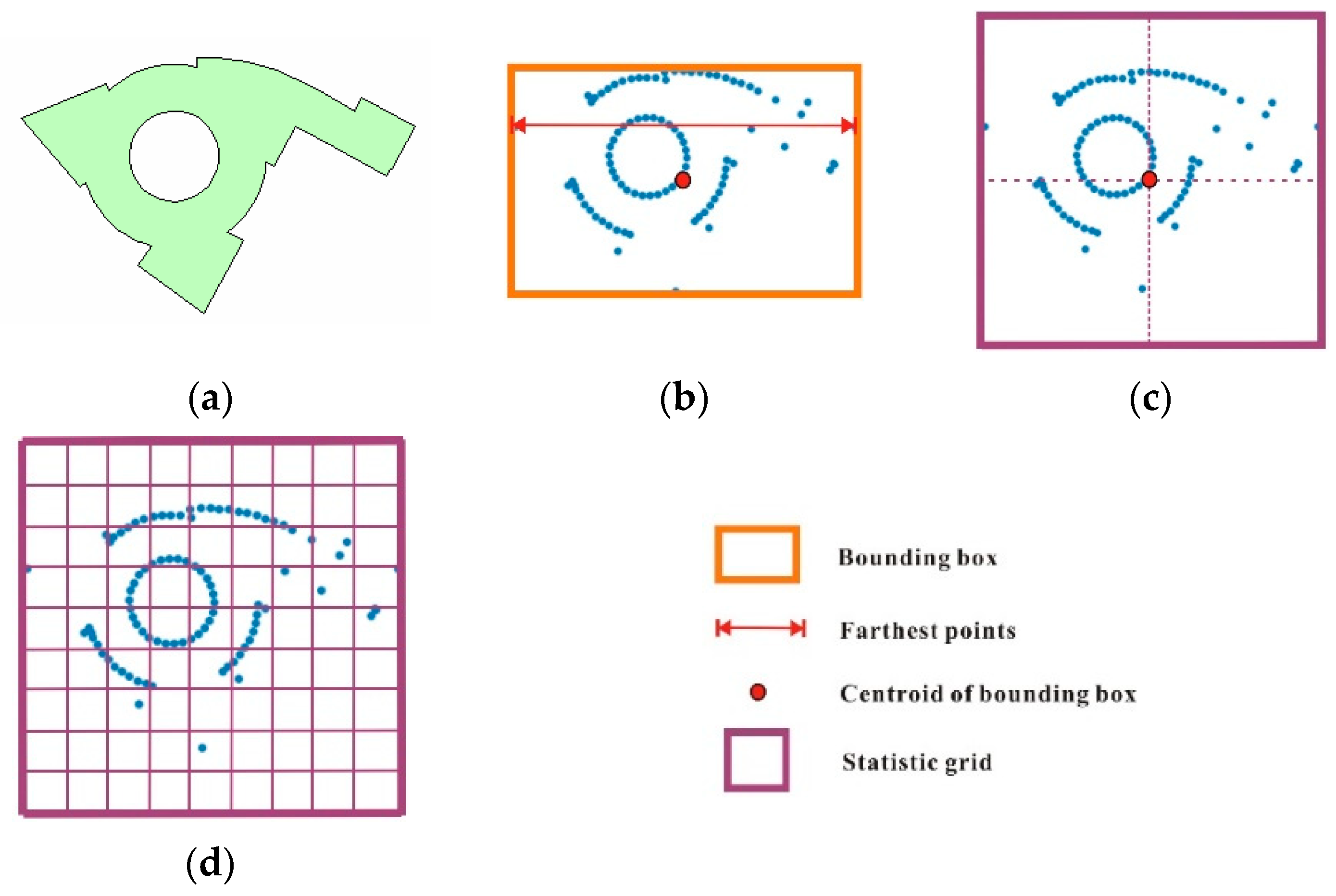
2.1.2. Derivation of Grid Context Information

Shape is represented by a set of vertices and interpolation points. Belongie et al. introduced a local shape descriptor named the shape context [16]. The shape context, at a point, captures the distribution of adjacent points the describing relative position of other shape points. Although the existing shape context descriptor considers the relative positions of interpolation points, crucial information on the regional morphological features, such as the elongation and curvature, is not preserved. As the interpolation points are mapped into the cell of a statistic grid with similar context information, the cells are regarded as proxies of the sampling points to extract context information efficiently. Meanwhile, the arrangement of cells in the statistic grid represents the relative positions of the sampling points of the contour. The arrangement is reflected by the relative direction and distance between a cell and neighboring cells. To enhance the shape discrimination by incorporating multiscale statistic features, a grid context descriptor is introduced to encode the context information representing local relative positions and morphological features of interpolation points.

The grid context, which records the coarse arrangement of the rest of the shape with respect to the cell, refers to an efficient representation of the relative positions of the interpolation points of the contour. The arrangement of the interpolation points of the contour captures local information in detail. However, the grid context information of adjacent cells is so small that partial context information is redundant (Figure 5). Therefore, a grid context feature descriptor is proposed to encode the local distribution of contour points.

The first step in obtaining the context information of cells is identifying the range of the grid context. To trade-off between the efficiency of context feature extraction and the completeness of context information, a certain range was determined for a sliding template with a resolution of 5 on the statistical grid. In the second step, a sequence of context features of each cell was obtained by using the template to traverse the statistical grid and record value of the grid corresponding to the template. Finally, the shape context description of each sample cell was generated. However, a sequence of sparse context features cannot reflect the global structure of the shape. In addition, it is difficult to compare sparse grid context information directly. Therefore, contextual information must be condensed to generate a discriminative representation for comparison.

Based on the idea of convolution in image processing, a sparse matrix reflecting context information can be compressed into a dense form. The convolution kernel weights reflect the potential relative orientation and distance of each element in the rectangular template to the center cell of the convolution kernel. Thus, the design of the convolution kernel determines the degree of the contributions of adjacent cells to the grid context. These features store important context information, which is easier to process and compare. To ensure that the grid context blend feature of statistic grids with different resolutions maintains the consistency of corresponding detail information, the convolution kernel dimensions should be adjusted according to the size of the statistic grid. The size of the convolution kernel used in this study was defined as 5 × 5.

$$w_i=\{\begin{array}{c}\frac{I{d}_i\left(x\right)}{{{\displaystyle \sum }}_{i=1}^{N}I{d}_i\left(x\right)}, if d\left({cell}_i,{cell}_{center}\right)\ne 0\\ 0\hspace{1em}\hspace{1em}, if d\left({cell}_i,{cell}_{center}\right)=0\end{array},$$

(3)

$$I{d}_i\left(x\right)=\frac{1}{d{\left({cell}_i,{cell}_{center}\right)}^2},$$

(4)

$$d\left({cell}_i,{cell}_{center}\right)=max\left\{\left|x_i-x_{center}\right|,\left|y_i-y_{center}\right|\right\},$$

(5)

where $d_i$ is the distance between the i-th cell and centre cell of the kernel and $w_i$ is the generalized weight value of the i-th cell in a convolution kernel. N is the total number of cells in a kernel. To preserve context information in the convolution calculation and remove the influence of the central cell, the value of the central cell of the kernel is set to 0 (Figure 6a). To avoid the shrinking of the statistical grid after the convolution calculation, two rows of grid cells with a statistical value of 0 in the upper and lower ends of the statistical grid were padded. Subsequently, two columns of grid cells with a statistical value of 0 were padded on the left and right.

In contrast to traditional convolution filters, such as Sobel and Canny operators, the IDW convolution kernel is designed to enrich the edge characteristics rather than to simplify the edge information. Based on the corresponding color bar (Figure 6e), the richness of the edge feature can be observed after the convolution. A bright color represents strengthened information about vertices of the shape. After the convolution, the sparse and redundant grid context information was condensed into texture information, representing a discriminative visual pattern. Therefore, we can use more efficient texture characteristics analysis methods to compare shape features.

2.2. Calculation of the Similarity

Julesz et al. proposed that humans use texture fields as a vision discriminator [22]. To obtain shape similarity calculation results that are consistent with human perception, texture information was used to distinguish the differences between the statistic grid of polygons in this section. Based on the shape representation results of multiscale grids, a texture descriptor was introduced to construct the feature tensor in Section 2.2.1. Subsequently, the correlation coefficients between any two feature tensors were calculated to measure the shape similarity of the two polygons in Section 2.2.2.

2.2.1. Extraction of Multiscale Texture Features

The texture information reflected by the condensed grid context information can be used to discriminate the different shapes. Researchers have proposed statistic-, spectral-, and structure-based approaches to measure the differences between the texture features of images and extract texture information. Because structure-based methods are susceptible to statistical grid rotation and scaling, we chose the grey level co-occurrence matrix (GLCM), a statistic-based method, to extract texture features with rotation invariance and low computational complexity.

The GLCM is defined as the co-occurrence distribution matrix of a pair of pixel values at a given offset, which is the pixel distance d in a specific direction $\theta$. Generally, the direction $\theta$ is set to 0°, 45°, 90°, and 135°. Because the application of a large pixel distance to a fine texture would yield a GLCM that does not capture detailed texture information, the pixel distance d is usually set to 1.

The number of grey levels is an important factor in GLCM computation because the computational complexity of the GLCM method is highly sensitive to the number of grey levels [23]. Although more levels yield more accurate extracted texture information, the resulting high sparsity of the GLCM would increase the computational costs. However, a decrease in the grey level to reduce the sparsity will lead to the loss of spatial dependence information. In this paper, to keep balance between accuracy and efficiency, the number of grey levels n was set to 10 after a set of tests.

Although Haralick et al. introduced 13 statistics to extract texture features from the GLCM to discriminate different texture patterns [24], Ulaby et al. reported that only four features (contrast, inverse difference moment, correlation, and sum of squares) are independent of each other in the remote sensing data [25]. Based on this statistical separability analysis, Gadkari selected the angle second moment (ASM) and entropy features as the two best texture features for the image classification experiment [26]. Because the sum of squares strongly correlates with the angle second moment, we finally selected five statistics (contrast, inverse difference moment, correlation, angle second moment, and entropy) to determine the texture features.

The contrast (CON) reflects the sharpness of the texture and measures the number of local variations. The inverse difference moment (IDM) was used to measure local variations and the uniformity of the texture. The correlation (COR) measures the similarity of the GLCM elements in a row or column. The COR value reflects the intensity of the local greyscale correlation in a particular direction. The ASM is a measurement of the uniformity of the grey level of the texture. The entropy (ENT) measures the disorder or complexity of the texture.

Although it is easy to intuitively describe the texture with the statistic-based method, the extracted information still suffers from the limitation that it does not contain structure information regarding the gradient orientation of the pixels [27]. Therefore, the texture features calculated at the global scale do not have sufficient shape recognition capabilities. Because the direction of the farthest points of the polygon is parallel to the side of the statistical grid, the structural information significantly changes with an increase in the size of the sampling subregions in the diagonal direction. To enrich the structural information, rectangular sampling subregions are set up in the diagonal direction. Thus, multiscale texture feature tensors can reflect texture structure information for four directions from the outside to the inside. In addition, multi-resolution sampling subregions are constructed to provide local and global texture features to improve the recognition capability of the multiscale texture feature.

To maintain both local and global texture details in the three statistical grids with different resolutions, the sampling subregions were designed for different sizes [28]. Subregions sampled at multiple scales can enhance the recognition performance, but the amount of redundant information also increases based on the high similarity of texture features of adjacent scales. To balance information and reduce the amount of redundant data, we set the sampling sizes for the three statistical grids with different resolutions to four equidifferent scales of texture sampling frames.

The multiscale texture feature tensor was then constructed for the condensed grid context information generated by the four sampling subregions in each diagonal direction (A, B, C, and D) (Figure 7a). The four sampling subregions at equidifferent scales (Figure 7b). The texture features of the GLCM in each direction were calculated based on the sampling subregions of the statistic grid selected above (Figure 7c). Finally, based on the statistical grids of the three resolutions, a multiscale texture feature tensor with five dimensionalities (3 grid resolutions × 4 diagonal directions × 4 sample regions × 4 texture directions × 5 texture descriptors) was constructed.

2.2.2. Calculation of the Shape Similarity

As an effective index reflecting the consistency of the trends of dependent variables with varying independent variables, the Pearson correlation coefficient was employed to measure the similarity between two series of texture feature tensors. To eliminate repetitive comparisons of feature tensors from sampling subregions with the same size, four texture feature matrices (4 × 5) of the different texture directions were superposed and combined into an extended feature matrix (16 × 5). The comparison of the feature tensors can be divided into three stages. In the first stage, the correlation coefficient between the corresponding texture descriptor of two extended feature matrices is calculated. In the second stage, the texture information of the sampling subregions with four different sizes is compared. In the third stage, the texture information of the three statistical grids is compared. Based on the structure of the multiscale texture tensor, the average correlation coefficient of the texture features is calculated in the bottom-up order. The equation for the calculation of the similarity for the comparison of the two texture feature tensors S and Q is as follows:

$$Similarity\left(S,Q\right)=\frac{1}{\mathrm{M}}\times {{\displaystyle \sum }}_{k=1}^3\left(\frac{1}{4}\times {{\displaystyle \sum }}_{j=1}^4\left(\frac{1}{5}\times {{\displaystyle \sum }}_{i=1}^{5}Corr\left({tensor}_{S_k}^{i,j},{tensor}_{Q_k}^{i,j}\right)\right)\right),$$

(6)

where $S_k$ and $Q_k$ represent the grid context information of the statistical grid at the k-th resolution of the two shapes. In the characteristic tensor, ${tensor}_{S_k}^{i,j}$ is the i-th texture feature at the j-th sampling scale. The parameter M is set to 3.

As mentioned in Section 2.1.1, the external contour features of the compared polygons can be aligned based on the polygon rotation determined by the main direction of the external contour. However, for the holed polygons, the alignment of the internal contour is as important as the alignment of the external contour. For example, in two-holed polygons with the same external contour but dissimilar internal contour, the inner contour is not in the corresponding position (Figure 8), although the main directions of the two polygons are rotated. Therefore, the calculated shape similarity is incorrect. To eliminate the inconsistency regarding the feature position, we adjusted the statistical grid with a 90° clockwise rotation around the center of the statistical grid. Subsequently, we performed and recorded symmetrical transformations of the rotated statistic grids. To obtain eight statistical grids, the corresponding eight texture feature tensors can be generated. The eight feature tensors of the obtained sample pattern and that of the reference pattern were calculated to determine the similarity. The maximum value among the eight calculation results was used as the similarity between the two polygons.

3. Experimental Results

In this section, we first evaluate the sensitivity of the proposed method to the gradual evolution of a polygon contour. Subsequently, we validate the performance of the proposed calculation of the shape similarity for holed and non-holed polygons to illustrate the advantages of the proposed method. Lastly, we compare our method with two common methods using standard building footprint datasets.

3.1. Test of the Sensitivity to Contour Variation

To test the sensitivity of the shape similarity measurement model to the change of the polygon contour, Victoria Nyanza (polygon A) in southern Africa and the Nidaros Cathedral (polygon B) in Norway were used as example data. Polygon A derived from the Natural Earth vector dataset is a holed polygon with 15 holes, while polygon B derived from the OSM building footprint dataset is a non-holed polygon. To obtain a set of generalized polygons with different levels of details, the Wang–Müller algorithm was employed to simplify the contours by eliminating insignificant bends [29]. In this study, four tolerances were used to determine the diameter of a circle that approximates a significant bend (Figure 9).

The sensitivity of the quantification of minute variations between polygon contours is a crucial effectiveness criterion for the shape similarity measurement method. From the perspective of human vision, basic morphology features are sufficient to identify different types of shapes. Thus, generalized polygons are generally regarded to be similar shapes, while subtle differences between generalized polygons are ignored (Figure 9). However, in practical applications, such as the retrieval of global building footprints, the identification of subtle differences in contours is the key to drawing conclusions. The algorithm must be sensitive such that the calculated similarity shows a consistent trend with the change of the contour. As the generalized polygons are derived from the original polygon, the basic morphology features of simplified polygons are maintained. The differences between the similarities caused by the contour variation of the shapes should be within a reasonable range. Therefore, the sensitivity must be verified from both tendency consistency and rationality aspects.

To identify the sensitivity of the proposed method, the shape similarity between generalized polygons was calculated and the consistency between the tendency of the similarity variation and incensement of tolerance was determined. The shape similarity between the generalized polygons of polygons A and B was calculated, as shown in

Table 1. Sensitivity test result for polygon A.

Shape Similarity		Original Polygon	Tolerance
			3 m	10 m	20 m	35 m
Original polygon		1.00	0.90	0.82	0.75	0.72
3 m		0.90	1.00	0.85	0.77	0.76
10 m		0.82	0.85	1.00	0.77	0.78
20 m		0.75	0.77	0.77	1.00	0.91
35 m		0.72	0.76	0.78	0.91	1.00

and

Table 2. Sensitivity test result for polygon B.

Shape Similarity		Original Polygon	Tolerance
			5 km	10 km	15 km	20 km
Original polygon		1.00	0.90	0.86	0.80	0.78
5 km		0.90	1.00	0.86	0.79	0.77
10 km		0.86	0.86	1.00	0.82	0.80
15 km		0.80	0.79	0.82	1.00	0.86
20 km		0.78	0.77	0.80	0.86	1.00

. The similarities between the original polygon and generalized polygons decrease with increasing tolerance. Compared with the original polygon, the simpler generalized polygon preserves less contour detail. With increasing differences in the contour details, the shape similarity notably decreases. This illustrates that the proposed method is consistent.

In addition to the consistency, the similarity rationality is also a critical factor of the sensitivity validation. The shape similarity between two generalized polygons with similar tolerances is higher than that of generalized polygons with larger tolerances, as shown in Table 1 and Table 2. This illustrates that the shape similarity measurement method is independent of the degree of contour simplification. In addition, the calculated shape similarity only depends on the difference between the two polygon outlines. Thus, the differences between the similarities are within a reasonable range. To sum up the above-mentioned results, the similarity measurement method is sensitive to the variation of the contour, which means that subtle shape differences can be captured.

3.2. Similar Polygon Retrieval Test

To validate the performance of the proposed method, a holed polygon A and non-holed polygon B were chosen from two real scenarios in Munich, Germany (Figure 10 and Figure 11). The proposed method was then applied to determine footprints with similar shapes and sizes. Scenario A is the Max-Planck-Institut für Physik in the Studentenstadt Freimann. Scenario B is Hasenbergl-Lerchenau Ost in Feldmoching-Hasenbergl, which is a borough in the northern part of Munich. The building footprints of these scenarios were derived from the OSM dataset. Scenarios A and B contain 131 and 1183 building footprints, respectively (Figure 11).

The identification of polygons with similar shapes plays an important role in GIS applications. For example, it can be applied in the spatial analysis of mining building patterns. Thus, an accurate and complete similar shape cognition result is the basis for further spatial analysis. To validate the accuracy and completeness of the cognition result and test the performance of our method, we used the evaluation indexes ‘precision’ and ‘recall’. In this study, the precision was regarded to be the ratio of the number of similar polygons corresponding to human cognition to the number of retrieved polygons. The recall was regarded to be the ratio of the number of similar polygons corresponding to human cognition to the number of all relevant polygons of a scenario.

3.3. Comparison with the Turning Function and Fourier Descriptor Methods

Because the evaluation of the shape similarity of polygons is relatively subjective, the calculated shape similarity should conform to human cognition. Thus, researchers generally determine if a method is available according to the correctness of human cognition. Ai et al. employed 20 reference and 6 template building footprints to validate the advantages and disadvantages of the Fourier descriptor (F-model) and turning function (T-model) [30]. Both the Turning function [31] and Fourier descriptor [1] are widely used in GIS to calculate the shape similarity of polygons. Therefore, we used the same building footprints to compare the method proposed in this paper with the TF and Fourier methods.

Based on the template and reference polygons used in the previous study, as shown in the experimental data above, the similarity between each reference and template building footprint was calculated using the contour diffusion method (C-model). The same form of matrix was obtained for the shape similarity, as shown in

Table 3. Shape similarity between the template and reference building footprints and human recognition result.

Reference Building Footprints	Template Building Footprints						Recognition Correct?
	0.76	0.46	0.31	0.40	0.55	0.40	Yes
	0.47	0.78	0.43	0.58	0.65	0.62	Yes
	0.79	0.33	0.38	0.36	0.53	0.37	Yes
	0.25	0.44	0.70	0.76	0.60	0.28	Yes
	0.41	0.90	0.43	0.54	0.63	0.65	Yes
	0.57	0.54	0.65	0.87	0.74	0.44	Yes
	0.52	0.54	0.66	0.89	0.71	0.42	Yes
	0.37	0.47	0.76	0.66	0.46	0.35	Yes
	0.54	0.56	0.65	0.88	0.74	0.44	Yes
	0.41	0.78	0.41	0.54	0.64	0.61	Yes
	0.79	0.42	0.30	0.42	0.53	0.45	Yes
	0.63	0.58	0.46	0.68	0.88	0.50	Yes
	0.86	0.42	0.43	0.53	0.68	0.50	Yes
	0.44	0.66	0.35	0.29	0.54	0.67	Yes
	0.75	0.52	0.42	0.40	0.53	0.47	Yes
	0.75	0.36	0.31	0.40	0.50	0.43	Yes
	0.47	0.51	0.65	0.81	0.67	0.39	Yes
	0.64	0.33	0.36	0.28	0.47	0.41	Yes
	0.52	0.75	0.38	0.48	0.63	0.60	Yes
	0.50	0.57	0.46	0.56	0.74	0.56	Yes

. Among the 20 reference building footprints, all elements are correctly recognized as being similar to templates that are consistent with human cognition. Thus, the recognition correctness of the contour diffusion method is 100%. Compared with the correctness of the TF method (80%) and Fourier method (85%), the contour diffusion method agrees more with human cognition.

4. Discussion

In this section, we discuss optimal parameter selection for the contour diffusion method and the limitations of this shape similarity measurement approach. The proposed similarity measurement method might be affected by the following factors.

4.1. Optimal Parameter Selection for the Contour Diffusion Method

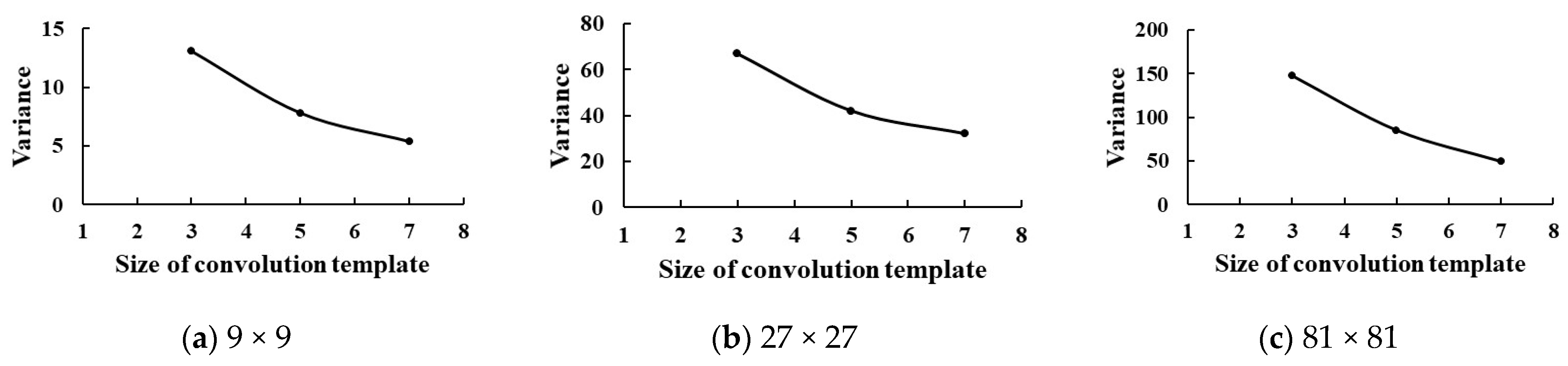
4.1.1. Size of the Convolution Template

Based on the convolution operation, the grid context information of the contour can be condensed from a statistic grid with a different size. However, a too-small convolution template causes the loss of context information. A too-large convolution template causes redundancy. To identify the optimal convolution template size for different statistic grid sizes, we first built three sizes of convolution kernels for the three statistical grids with different resolutions (Figure 12).

Because the weight elements of the kernel are determined by the inverse distance weight approach, the size affects the analysis range of the context information and the shape feature depicted in the corresponding statistic grid. To identify the effects of different convolutional kernels on the shape features expressed by statistical grids, each convolution kernel was used to convolute three statistic grids with different sizes. To quantify the salience of the shape features, the variance was chosen as the evaluation index. The variance of each convolution result was calculated and recorded (Figure 13).

An extremely large convolution kernel size would cover most cells of a 9 × 9 statistic grid, leading to a weakened shape feature (without identification) (Figure 14c). In contrast, an ultra-small kernel size causes the context information of an 81 × 81 statistic grid to merely reflect the micro-range of the contour, disregarding the structural information of the shape (Figure 14g). The variance of statistic grids with different resolutions decreases with increasing kernel size. A high variance indicates that the cell value of the convolution result fluctuates greatly around the average. The shape features represented by the convolution results are still notable. A low variance implies that the dispersion degree of the cell value of the convolution result is small. The shape features represented by the convolution results are not notable. To consider both an appropriate range of the context and shape feature significance, IDW5 was chosen as the convolution kernel.

4.1.2. Interpolation Points

Because the number of interpolation points influences the condensed grid context feature obtained after the convolution operation, we performed a sensitivity analysis of the interpolation points for the diffusion matrix at different scales. Because the Shannon entropy is a basic metric associated with any random variable, which can be interpreted as the average level of ‘information’ and ‘uncertainty’ included in the variable [32], we calculated the Shannon entropy of the matrix elements of the condensed grid context feature and used the different interpolation points and their corresponding information entropy as two variables to draw a line graph. The results show that the Shannon entropy enters a weak fluctuation state with increasing numbers of interpolation points when the matrix of the three scales obtained by different templates increases to a certain number. We assume that the number of interpolation points that will reach a steady state is the number of optimal interpolation points of the current scale (Figure 15).

Figure 15 shows that the entropy change of small-scale statistic grids is stable when the number of interpolation points is about 1500. The entropy changes of a middle-scale statistic grid stops fluctuating when the number of interpolation points is about 5000. Because the entropy value of large-scale statistic grids does not stabilize due to large fluctuations, we selected the lowest slope point of 10,000 as a stable tendency. Therefore, we used 1500, 5000, and 10,000 as the optimal number of interpolation points for the three scales, respectively.

4.2. Limitation of the Similarity Cross-Comparison

Based on the experimental result demonstrated in Section 3.1, the proposed method is sensitive to the variation of a contour of man-made and natural objects. The performance test in Section 3.2 validated the accuracy and completeness of the search results. However, there is still one limitation; that is, the shape similarity calculated by the proposed method cannot be used for the similarity cross-comparison. This means that although polygons A and B have a shape similarity similar to that of polygon C, polygons A and B cannot be considered to be similar polygons, as shown in

Table 4. Shape similarity between the template and reference building footprints and human recognition result.

Shape Similarity		Polygon A	Polygon B	Polygon C
Polygon A		1	0.51	0.50
Polygon B		0.51	1	0.43
Polygon C		0.50	0.43	1

. Therefore, to identify similar polygons for each polygon, all polygons must be compared with each other. This limitation leads to a certain degree of redundancy in the calculation.

Although the proposed method can be used to identify most of the building footprints with similar shapes, the precision is not satisfactory. This is due to the polygon size, which is also an important factor in the retrieval of building footprints by human intuition. For example, scenario A contains many rectangular building footprints, which have a high shape similarity with sample polygon A. However, because of their different sizes, they still cannot be retrieved as similar building footprints by the human eye.

5. Conclusions

In this paper, a contour diffusion method based on the multiscale feature is proposed to combine external and internal contour features. To obtain an intuitive result, we propose a way to represent the shape feature in combination with the multiscale statistic feature and grid context information based on the Gestalt psychology theory on human hierarchical cognition [33].

The grid context information provides a wealth of texture information. As an important visual cognition clue, the texture feature analysis method leads to a shape similarity calculation result that agrees more with human cognition. The grid context descriptor can be used to convey the contour features to the grid by convolution. The similarity calculation equation compares the feature tensor between sample and reference polygons.

The results show that the method based on the multiscale feature is an effective similarity measuring tool for polygons in the geographic domain. It has three advantages over existing shape similarity measurement approaches. First, we consider both contour and region feature when measuring the shape similarity. Secondly, the use of texture descriptors to express shape features agrees more with human cognitive habits. Finally, the accuracy of the proposed method is superior to that of the turning function and Fourier descriptor, which are two popular techniques used for the measurement of the shape similarity. In this study, we consider only holed polygons and non-holed polygons, and in the future multi-polygons should be tested to enhance the universality of this shape measurement approach. Meanwhile, in addition to accuracy, the efficiency should also be regarded as a critical index for judging the performance of shape similarity measurement approach in future research. In shape retrieval and pattern matching applications, online real-time calculations can be achieved.

References

1. Xu, Y.; Xie, Z.; Chen, Z.; Wu, L. Shape similarity measurement model for holed polygons based on position graphs and Fourier descriptors. Int. J. Geogr. Inf. Sci. 2017, 31, 253–279. [Google Scholar] [CrossRef]
2. Yan, X.; Ai, T.; Yang, M.; Yin, H. A graph convolutional neural network for classification of building patterns using spatial vector data. ISPRS J. Photogramm. Remote Sens. 2019, 150, 259–273. [Google Scholar] [CrossRef]
3. Chen, Z.; Zhu, R.; Xie, Z.; Wu, L. Hierarchical model for the similarity measurement of a complex holed-region entity scene. ISPRS J. Photogramm. Remote Sens. 2017, 6, 388. [Google Scholar] [CrossRef] [Green Version]
4. Wang, X.; Burghardt, D. A typification method for linear building groups based on stroke simplification. Geocarto Int. 2019, 1–20. [Google Scholar] [CrossRef]
5. Kurnianggoro, L.; Wahyono; Jo, K.H. A survey of 2D shape representation: Methods, evaluations, and future research directions. Neurocomputing 2018, 300, 1–16. [Google Scholar] [CrossRef]
6. Yan, X.; Ai, T.; Yang, M.; Tong, X. Graph convolutional autoencoder model for the shape coding and cognition of buildings in maps. Int. J. Geogr. Inf. Sci. 2021, 35, 490–512. [Google Scholar] [CrossRef]
7. Clementini, E.; di Felice, P. A global framework for qualitative shape description. Geoinformatics 1997, 1, 11–27. [Google Scholar] [CrossRef]
8. Freeman, H.; Saghri, A. Generalized chain codes for planar curves. In Proceedings of the 4th International Joint Conference on Pattern Recognition, Kyoto, Japan, 7–10 November 1978; pp. 701–703. [Google Scholar]
9. Arkin, E.M.; Chew, L.P.; Huttenlocher, D.P.; Kedem, K.; Mitchell, J.S.B. An efficiently computable metric for comparing polygonal shapes. IEEE Trans. Pattern Anal. Mach. Intell. 1990, 13, 209–216. [Google Scholar] [CrossRef] [Green Version]
10. Elghazal, A.; Basir, O.; Belkasim, S. Farthest point distance: A new shape signature for Fourier descriptors. Signal. Proc. Image Commun. 2009, 24, 572–586. [Google Scholar] [CrossRef]
11. Huang, M.; Lin, J.; Chen, N.; An, W.; Zhu, W. Reversed sketch: A scalable and comparable shape representation. Pattern Recognit. 2018, 80, 168–182. [Google Scholar] [CrossRef]
12. Yasseen, Z.; Verroust-Blondet, A.; Nasri, A. Shape matching by part alignment using extended chordal axis transform. Pattern Recognit. 2016, 57, 115–135. [Google Scholar] [CrossRef]
13. Schmidhuber, J. Deep learning in neural networks: An overview. Neural Netw. 2015, 61, 85–117. [Google Scholar] [CrossRef] [PubMed] [Green Version]
14. Teague, M.R. Image analysis via the general theory of moments. J. Opt. Soc. Am. 1980, 70, 920–930. [Google Scholar] [CrossRef]
15. Lu, G.; Sajjanhar, A. Region-based shape representation and similarity measure suitable for content-based image retrieval. Multimed. Syst. 1999, 7, 165–174. [Google Scholar] [CrossRef]
16. Belongie, S.; Malik, J.; Puzicha, J. Shape matching and object recognition using shape contexts. IEEE Trans. Pattern Anal. Mach. Intell. 2002, 24, 509–522. Available online: https://ieeexplore.ieee.org/document/993558 (accessed on 14 February 2021). [CrossRef] [Green Version]
17. Žunić, J.; Hirota, K.; Rosin, P.L. A Hu moment invariant as a shape circularity measure. Pattern Recognit. 2010, 43, 47–57. [Google Scholar] [CrossRef]
18. Fu, Z.; Fan, L.; Yu, Z.; Zhou, K. A moment-based shape similarity measurement for areal entities in geographical vector data. ISPRS J. Photogramm. Remote Sens. 2018, 7, 208. [Google Scholar] [CrossRef] [Green Version]
19. Xu, Y.; Xie, Z.; Chen, Z.; Xie, M. Measuring the similarity between multipolygons using convex hulls and position graphs. Int. J. Geogr. Inf. Sci. 2020, 1–22. [Google Scholar] [CrossRef]
20. Wagemans, J.; Elder, J.H.; Kubovy, M.; Palmer, S.E.; Peterson, M.A.; Singh, M.; von der Heydt, R. A century of Gestalt psychology in visual perception: I. Perceptual grouping and figure-ground organization. Psychol. Bull. 2012, 138, 1172. [Google Scholar] [CrossRef] [Green Version]
21. Shapiro, L.G.; Stockman, G.C. Computer Vision; Prentice Hall: Hoboken, NJ, USA, 2001. [Google Scholar]
22. Julesz, B.; Gilbert, E.N.; Victor, J.D. Visual discrimination of textures with identical third-order statistics. Biol. Cybern. 1978, 37, 137–140. [Google Scholar] [CrossRef]
23. Clausi, D.A. An analysis of co-occurrence texture statistics as a function of grey level quantization. Can. J. Remote Sens. 2002, 28, 45–62. [Google Scholar] [CrossRef]
24. Haralick, R.M.; Shanmugam, K.; Dinstein, I.H. Textural features for image classification. IEEE Trans. Syst. Man Cybern. 1973, 6, 610–621. [Google Scholar] [CrossRef] [Green Version]
25. Ulaby, F.T.; Kouyate, F.; Brisco, B.; Williams, T.L. Textural information in SAR images. IEEE Trans. Geosci. Remote Sens. 1986, 24, 235–245. [Google Scholar] [CrossRef]
26. Gadkari, D. Image Quality Analysis Using GLCM. Master’s Thesis, University of Central Florida, Orlando, FL, USA, 2004. [Google Scholar]
27. Fu, Z.; Qin, Q.; Luo, B.; Wu, C.; Sun, H. A local feature descriptor based on combination of structure and texture information for multispectral image matching. IEEE Geosci. Remote Sens. Lett. 2018, 16, 100–104. [Google Scholar] [CrossRef]
28. LaMar, E.; Hamann, B.; Joy, K.I. Multiresolution Techniques for Interactive Texture-Based Volume Visualization; IEEE: San Francisco, CA, USA, 1999. [Google Scholar]
29. Wang, Z.; Müller, J.C. Line generalization based on analysis of shape characteristics. Cartogr. Geogr. Inf. Syst. 1998, 25, 3–15. [Google Scholar] [CrossRef]
30. Ai, T.; Cheng, X.; Liu, P.; Yang, M. A shape analysis and template matching of building features by the Fourier transform method. Comput. Environ. Urban. Syst. 2013, 41, 219–233. [Google Scholar] [CrossRef]
31. Fan, H.; Zipf, A.; Fu, Q.; Neis, P. Quality assessment for building footprints data on OpenStreetMap. Int. J. Geogr. Inf. Sci. 2014, 28, 700–719. [Google Scholar] [CrossRef]
32. Shannon, C.E. A mathematical theory of communication. ACM SIGMOBILE Mob. Comput. Commun. Rev. 1948, 5, 3–55. [Google Scholar] [CrossRef]
33. Jackson, I. Gestalt—A learning theory for graphic design education. Int. J. Art Des. Educ. 2008, 27, 63–69. [Google Scholar] [CrossRef]
Figure 1. Workflow of the shape similarity measurement.
Ijgi 10 00279 g001
Figure 2. Orientation standardization. (a) Original polygon, (b) Vertices of the polygon before rotation, and (c) Vertices of the polygon after rotation.
Ijgi 10 00279 g002
Figure 3. Generation of the statistic grid. (a) Rotated polygon, (b) Farthest points of the polygon vertices, (c) Centroid of the bounding box, and (d) 9 × 9 low-resolution statistic grid.
Ijgi 10 00279 g003
Figure 4. Extraction of the multiscale statistic feature. (a) Interpolation points, (b) Statistics for points covered by each cell, (c) 9 × 9 visualization statistical grid, (d) 27 × 27 visualization statistical grid, (e) 81 × 81 visualization statistical grid.
Ijgi 10 00279 g004
Figure 5. Representation of the grid context. (a) 27 × 27 visualization statistical grid, (b) Two adjacent cells marked in the statistical grid, (c) Redundant context information of adjacent cells.
Ijgi 10 00279 g005
Figure 6. Construction of contextual information using convolution. (a) Convolution kernel, (b) Extended statistic grid, (c) Condensed context information, (d) Visualization of the statistic grid, and (e) Visualization of condensed context information.
Ijgi 10 00279 g006
Figure 7. Extraction of the multiscale texture feature at middle resolution. (a) Four diagonal directions, (b) Four sampling subregions, (c) Four texture directions (0°, 45°, 90°, and 135°), and five texture descriptors (Asm, Con, Ent, IDM, and Corr).
Ijgi 10 00279 g007
Figure 8. Tensor alignment. (a) Two holed polygons, (b) Generation of eight corresponding texture feature tensors after rotation and symmetry, and (c) Aligned texture feature tensors.
Ijgi 10 00279 g008
Figure 9. Original polygons of the test entities. (a,b) are remote sensing images of two experimental objects.
Ijgi 10 00279 g009
Figure 10. Sample polygons for the test. (a) a holed polygon of scenario A. (b) a non-holed polygon of scenario B.
Ijgi 10 00279 g010
Figure 11. Shape similarity between sample polygons and other building footprints. (a) all the holed polygons in scenario A are found. (b) similar polygons in scenario B are found.
Ijgi 10 00279 g011aIjgi 10 00279 g011b
Figure 12. Three sizes of convolution kernels. (ac) the sum number of weights of IDW is 1.
Ijgi 10 00279 g012
Figure 13. Decrease of the variance with increasing kernel size. (ac) downtrend of variance is similar for different scale.
Ijgi 10 00279 g013
Figure 14. Condensed grid context feature for convolution templates with different sizes. (ai) IDW5 is the tradeoff between the richness of shape feature and the range of grid context information.
Ijgi 10 00279 g014
Figure 15. Entropy of the contour diffusion fluctuating with the increase in the number of interpolation points. (ac) When the number of interpolation points reaches the critical value, the entropy tends to be stable.
Ijgi 10 00279 g015