Spatial Distribution and Morphological Identification of Regional Urban Settlements Based on Road Intersections

Abstract

To measure and present urban size urban spatial forms, in solving problems in the rapid urbanization of China, urban territorial scope identification is essential. Although current commonly used methods can quantitatively identify urban territorial scopes to a certain extent, the results are displayed using a continuous and closed curve with medium- and low-resolution images. This makes the acquisition and interpretation of data challenging. In this paper, by extracting discretely distributed urban settlements, road intersections in OpenStreetMap (OSM), electronic maps, and urban expansion curve based on fractal thoughts have been used to present urban territorial scope and spatial form. Guangzhou, Chengdu, Nanjing, and Shijiazhuang cities were chosen as the identification targets. The results showed that the distance threshold corresponding to the principal curvature point of the urban expansion curve plays a vital role in the extraction of urban settlements. Moreover, from the analysis, the optimal distance thresholds of urban settlements in Guangzhou, Chengdu, Nanjing, and Shijiazhuang were 132 m, 204 m, 157 m, and 124 m, respectively, and the corresponding areas of urban territorial scopes were 1099.36 km², 1076.78 km², 803.07 km², and 353.62 km², respectively. These metrics are consistent with those for the built-up areas.

1. Introduction

Urbanization is inevitable the economic development of any country. According to data released by the National Bureau of Statistics of China, the urbanization rate in China reached 59.58% by the end of 2018 [1]. Urbanization not only facilitates socio-economic development, but it also accelerates the exposure of urban problems. The development of urban and rural areas can be unbalanced. Take for instance, in some areas in China, the rate of land urbanization has exceeded that of population urbanization, and resources have been consumed excessively. Moreover, degradation of the ecological environment and other problems are non-negligible in the context of urbanization. As a result, the sustainable development of cities is impeded significantly [2,3]. To solve these problems and to realize a scientific and sustainable urban development, many scholars have put forward new ideas: eco-city [4] and smart city [5]. To realize these ideas, the present situation of urban development needs to be understood, the size of cities also needs to be scientifically measured, planning and arrangements should be adjusted, and the blind expansion of cities should be regulated [6].

One of the prerequisites for measuring the urban size is the clear definition of urban boundaries and urban territorial scopes. Different definitions of urban boundaries directly affect the inferences from statistical analysis of urban activities. In urban geography, there are three key concepts for cities: city proper, urban agglomerations and metropolitan areas [7,8]. Urban agglomerations are sometimes replaced with urbanized areas [8,9]. Different urban concepts correspond to different urban boundaries and urban territorial scopes. When the territorial scope is effectively defined and the urban size is objectively determined, urban spatial information can be correctly extracted, and conclusions drawn from the spatial information can truly reflect urban characteristics [9].

The urban boundary and urban territorial scope, that is, the actual spatial scope of a city, are comprehensive concepts revolving around a variety of factors. Some of these factors include economy, society, population distribution, and geomorphological characteristics [10]. Many other related concepts such as central city area, main city area, built-up area, land for urban construction, downtown and administrative region of a city, etc. can be found in existing research works and applications [11,12]. Amongst these, the central city area, main city area, downtown, administrative region of a city, and land for urban construction are defined in terms of management functions as fixed areas. This is assuming that planning and policies remain unchanged and dynamic urban temporal and spatial changes are not reflected as a result [10,12]. The concept closest to the urban territorial scope is the built-up area. The built-up area is an official statistical index adopted in the China Urban Construction Statistical Yearbook that considers both temporal and spatial characteristics of built-up areas in cities [12], These characteristics are mainly obtained from local departments’ reports. The smallest statistical unit is the town. Although the built-up boundaries of cities may vary due to being in the form of data collected without the support of spatial scopes, they are still the official standard for national urban planning [12].

Scholars from various backgrounds have defined the urban boundary and urban territorial scope using different viewpoints. In a traditional sense, the urban boundaries mainly refer to the boundaries of administrative divisions or those defined subjectively by demographic data [13,14,15]. For example, the boundaries of administrative divisions are closely related to the urban planning scope that cannot truly reflect the actual development scope of the city [16,17]. At the same time, the data showing the boundaries of administrative divisions are mostly from the surveying department. The data often difficult to obtain due to their long cycle and poor shareability [14,15,18]. The statistical inferences drawn from urban and rural population are often dynamic [15,19]. As a result, the accuracy and timeliness of the analysis based on demographic data may also be limited [14,15]. To reflect the real urban boundaries and urban territorial scopes objectively and quantitatively as much as possible, multi-source remote sensing data and quantitative methods are widely used for urban boundary identification. To extract the urban boundaries, some scholars determined the optimal light threshold using Defense Meteorological Satellite Program (DMSP). Visible Infrared Imaging Radiometer Suite (VIIRS) night light data through spatial clustering, remote sensing interpretation, mutation detection and comparison of statistical data [20,21,22,23,24]. Other scholars also conducted research on urban boundary identification using alternative methods.

For example, Yao et al. [25] extracted and optimized the urban boundaries using vector data of small-scale residential areas based on triangulated irregular network (TIN). Tan and Chen [26] used remote sensing data to extract the urban boundaries based on spatial fusion algorithm and geographic information system (GIS). Lin et al. [17] explored the urban boundaries using electronic map points of interest based on kernel density estimation. However, the above methods all have their limitations. Zhang et al. proposed a semi-automatic method for the extraction of urban boundaries by using high-resolution images and geographical information data to combine urban landscape with morphological characteristics [27,28]. This method also integrates geographical knowledge with a series of normalization rules [27,28]. Gong et al. used satellite images with a resolution of 10 m, OSM, nighttime light, interest points, and Tencent social big data to generate the essential urban land use categories (EULUC), to depict the urban territorial scope [29]. The above methods are also defective in one way or another. The inherent excessive luminescence, or more specifically, the inherited blurring, in defense meteorological satellite program (DMSP)sensors and data management magnifies the apparent area of urban areas by 150–500%. Such a ratio becomes larger when it comes to smaller cities [24], with poor accuracy of products. Although this can be mitigated by visible infrared imaging radiometer (VIIRS)data to some extent, spatial details are still insufficient, and the determination of the optimal threshold still relies on subjective experience [24]. For the TIN method, spatial neighborhood fusion algorithm, and kernel density analysis are employed. Consequently, the selection of side length, threshold, and bandwidth is based on subjective experience. Therefore, the TIN method cannot be applied generically [18]. For the semi-automatic extraction method with high-resolution images, the results of urban boundaries need to be interpreted and revised manually in line with certain rules that are subjective and difficult to be repeatedly proved [27,28]. The data sources of EULUC in China are so vast that the processing is complicated. Since data were obtained in the early stage using inconsistent sampling standards. Due to the subjectivity of sample collection [29], it was challenging, in the process, to erase the accumulative errors and other errors resulting from multi-source data, leading to significant differences in accuracy of different cities.

In terms of the extraction of urban boundaries and urban territorial scopes, foreign scholars often identify the urban morphological boundaries and urban territorial scopes from a novel perspective, spatial self-organization [30,31,32,33,34,35,36]. There are four widely used methods, namely, the city clustering algorithm (CCA) proposed by Hernán et al. [37] and Rozenfeld et al. [38], the automatic identification method of urban settlement boundaries put forward by Chaudhry and Mackaness [39], the fractal-based method presented by Tannier et al. [18,40], and the approach to derive ”natural cities” by clustering street nodes/blocks, individual social media users’ locations or buildings locations developed by Bin Jiang and Tao Jia [14,35,41,42]. Bin Jiang and Tao Jia’s method (i.e., the fourth method) can be treated as a revised or an improved CCA. The first method is based on CCA, so it is necessary to set the buffer radius value (i.e., cluster resolution) in advance, and the prediction relies on subjective experience. For the second method, vector data at different scales which are not readily available are required. It is also difficult to guarantee the accuracy and timeliness of available vector data. For the third method, fractal geometry which is widely used in urban geography research is adopted, and several empirical studies and theoretical analyses have shown that urban morphology possesses fractal properties [34,43,44,45,46,47,48]. Even though the subjectivity in the research can be overcome from a fractal perspective [18,19], interpreting building vector data through the means of remote sensing images is a complicated process, and it is difficult to ensure its accuracy. For the fourth method, using road intersections to generate natural cities is mainly based on CCA. This requires the buffer radius value to be set in advance. Using social media users’ locations and buildings’ locations is based on the Head/Tail Breaks and the TIN method. Even though this avoids the subjective experience, it cannot accurately describe urban boundaries and lacks spatial details. Hence, it is more suitable for exploring the city distribution laws in a large space of a whole nation or even the world [27]. Particularly, there is currently no concept or definition of the urban boundary and urban territorial scope that is universally acknowledged [49]. Moreover, the results of the methods above are closely related to the selected data sources [27].

In the existing works on the urban boundary and urban territorial scope identification, almost all the results associated with urban boundary extraction can be expressed as a continuous closed curve between urban and rural areas. Since the effective influence scope of the geographic spatial interaction is directly restricted to the geographic bordering, the urban territorial scope can be determined. Because the urban territorial scope is continuously distributed in a certain space, an irrationality due to the lack of strict scientific verification exists [19,26]. It is very difficult or even impossible to draw a boundary with strict scientific significance between urban and rural areas [10,26]. The reason is that the city itself is a product of a certain historical stage, and the concept of the city is constantly changing under different historical conditions. More importantly, it is a gradual and interlaced process of transformation from the city to the countryside. Apparently, there is no obvious sign of the disappearance of the city and the emergence of the countryside [10]. The urban territorial scope is presented by a large and discretely distributed urban settlement composed of different geographical units in a certain space by effective spatial interactions, and such interactions are formed through geographic bordering and non-bordering [26].

To solve the above-mentioned problems, in this paper, the focus has been shifted from the identification of traditional and continuously closed urban boundaries and of the urban territorial scope to the identification of discretely distributed urban settlements in the space, with the aim of measuring the sizes of cities. From the research ideas of Jiang et al. [14] and Tannier et al. [18], open data including the OSM and electronic maps [50,51] with higher accuracy and wide applications in urban areas have been easily accessed and used. Intersections of urban vector road networks were extracted to substitute vector building data to avoid the subjective experience. The urban expansion curve based on fractal geometry was adopted to explore the distribution of regional urban settlements, and to identify the regional scopes and spatial distribution forms of cities. As a result, the staggered and discrete distribution of cities and rural areas in the space are displayed to provide new ideas for tackling the core of urbanization problems in China, that is, how to determine the urban territorial scope.

2. Materials and Methods

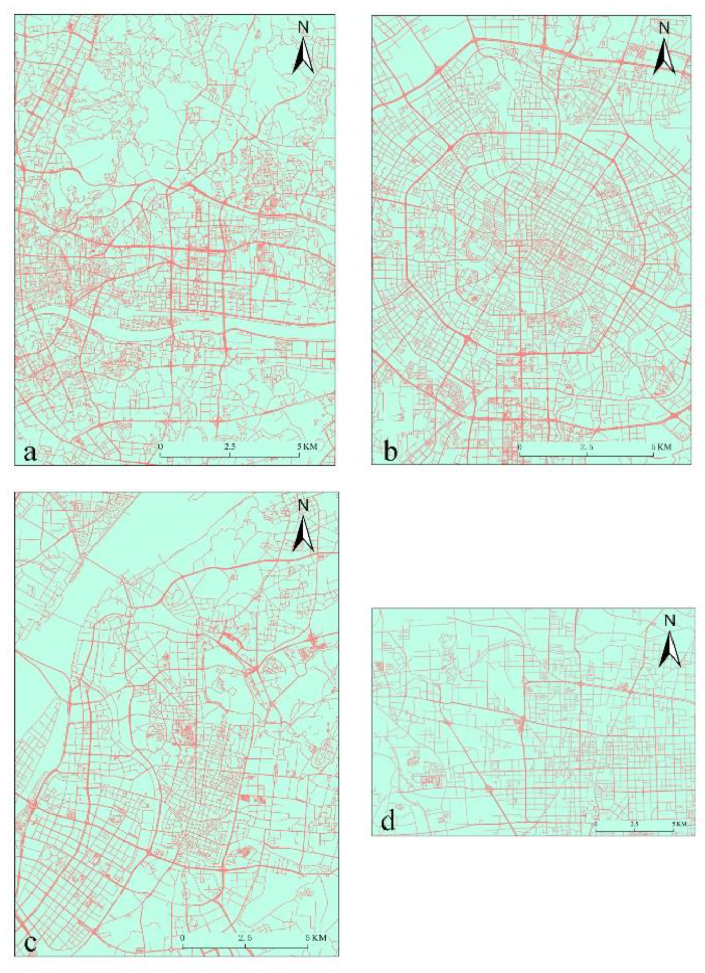
2.1. Research Regions and Data Sources

China has a large territorial area and with variances in her natural geographical environments. As a result, the selection of representative cities for exploring the spatial distribution of regional urban settlements is quite challenging. In this paper, the representative cities were selected based on the following criteria: (1) The cities are evenly distributed all over China. (2) The cities are characterized by large total economic output and a significant economic growth rate, which typify China’s urban development. (3) The cities are part of China’s traditional economic circles or large urban agglomerations, such as the Yangtze River Delta Economic Circle, the Pearl River Delta Economic Circle, and the Bohai Economic Circle. (4) Among the top 10% for the ranking of their urban built-up areas. Using these criteria, four cities (i.e., Guangzhou, Chengdu, Nanjing, and Shijiazhuang) were selected as the representative cities. The four representative cities are in the east, south, west and north of China, respectively. They all have a large urban size and possess representative urban spatial forms. Among them, Guangzhou (the central city of the Pearl River Delta Economic Zone) which is a traditional first-tier city [52] has its built-up area ranked as 3rd in China according to the China Urban Construction Statistical Yearbook 2018. Chengdu which is the first major city in the western region has a built-up area ranked as 6th in China. Nanjing (an important central city in the eastern Yangtze River Delta) which is an emerging quasi-first-tier city [52] has a built-up area ranked as 8th in China. Shijiazhuang (the first major city in the Beijing-Tianjin-Hebei region, except for Beijing and Tianjin) is a second-tier city [52], and its built-up area is ranked as 33rd in China. The method adopted in this paper is not restricted by territorial scopes [18]. The regional spatial scopes of the four cities were bounded by their administrative boundaries (including only municipal districts and excluding counties under city administration and county-level cities). All the administrative regions of Guangzhou (11 districts) and Nanjing (11 districts) were included. The territorial scopes of Shijiazhuang (eight districts, 11 counties, and three county-level cities) and Chengdu (11 districts, four counties, and five county-level cities) were too large compared with those of the other two cities. Moreover, the distance between remote counties or county-level cities and the downtown area was over 100 km. Due to the long distance between the territorial scope and the main city area, these counties or county-level cities are more like neighboring cities. Therefore, the regional scopes of counties and county-level cities of the two cities were removed, and only that of the main city area was selected, in an attempt to conform to the continuity of selected areas in Guangzhou and Nanjing [27,28]. The research spatial scope is between 500 km², and 4500 km², (see Figure 1).

The areas of human activities are connected by roads, and where there are roads, there are human footprints [14]. Road intersections are formed with connected and intersecting roads, and the region between adjacent intersections is the area of main human activities, ultimately forming urban regions. The smallest urban settlement also contains at least one road intersection. The denser the road intersections, the more frequent the city activities [14,15]. The road intersection data can be used to display the formation and evolution of urban settlements [14,19]. With the rapid development of Internet technologies, a vast number of data resources have been produced, and the effective use and mining of big network data has led to new research ideas [14,17]. OSM and electronic maps are the shared and innovative applications of map data [14,15,50,51,53,54,55]. Today, OSM data covers most of the cities in China, while electronic maps cover a larger area, including all urban areas in China. Road intersection data are an integral part of OSM and electronic maps, and they help limit the constraints of data on urban geography research [14,19]. In this paper, the street network data of the target city were extracted from OSM first [14,15], and then the single-layer road network data of the target city at a zoom level of 16, were obtained using electronic map application programming interface (API). With the combination of the two kinds of data, a complete urban road network was generated (see Figure 2). Finally, road intersections were extracted using GIS-based topological relationship among elements.

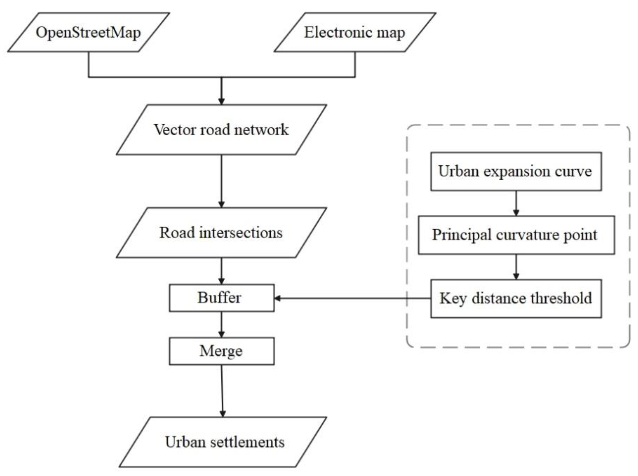
2.2. Research Methods

The method adopted in this paper mainly consists of three steps: (1) data preprocessing; (2) calculation of critical threshold; (3) extraction of urban settlements. The extraction of urban settlements is carried out as detailed in Figure 3. Firstly, the vector road network was obtained through OSM and electronic maps, and then the vector road network within the urban administrative region was figured out by using ArcGIS (ESRI, Redlands, CA, USA). This resulted in the creation of the set of road intersections. Secondly, the free software applications named Morphlim (https://sourcessup.renater.fr/morphlim/, accessed on 1 November 2020) [18,40] and ArcGIS were used to generate the urban expansion curve and to work out the principal curvature point and the key distance threshold. Finally, ArcGIS was used, with the key distance threshold as the buffer radius (to buffer and merge based on the set of road intersections) to obtain urban settlements.

2.2.1. Urban Expansion Curve

Tannier et al. [18] argued that the spatial organization structure within the city is like the fractal structure of Fourier Dusts, in which the actual city and street can be compared to black squares divided by white lines of a certain width. The number of white lines increases with the decrease in their respective widths. There is a strict hierarchical rule between the size and the number of white lines, and such a fractal feature can be measured by the Minkowski expansion method [56,57]. In other words, with the increase in the expansion buffer distance, the originally separated road intersections merge, and the urban settlements are gradually formed (see Figure 4). With further expansion, the number of urban settlements declines. Ultimately, all map spots merge, and the expansion terminates. The urban expansion curve is shown in Figure 5a, in which the horizontal axis indicates the expansion buffer distance, and the vertical axis indicates the number of urban settlements. According to fractal theory, the expansion buffer distance and the number of urban settlements conform to the power function law:

$$\mathrm{N}=\mathrm{a}{.r}^D$$

(1)

where N refers to the number of urban settlements, a is a constant, r refers to the expansion buffer distance, and D is the fractal dimension. If the logarithms of both sides of Equation (1) are taken simultaneously, the linear relation with D as the slope will be obtained (see Figure 5b)

$$\log \left(\mathrm{N}\right)=\mathrm{D}.log\left(\mathrm{r}\right)+log\left(\mathrm{a}\right)$$

(2)

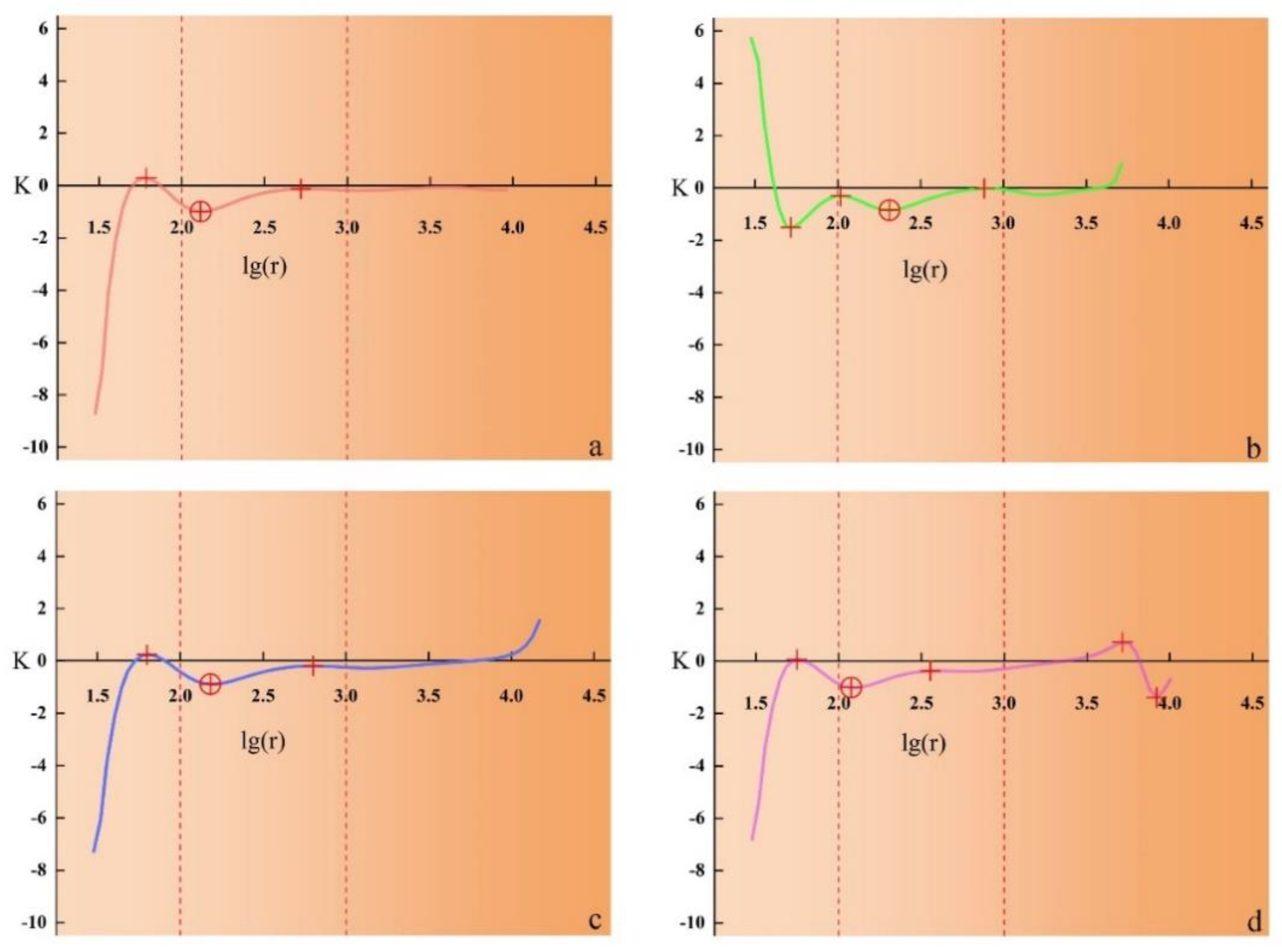
2.2.2. Principal Curvature Point of the Urban Expansion Curve

The density of urban entities is higher than that of rural entities, and the change rule of the number of settlements is very different between the two under the same distance threshold [26]. In this paper, the morphology of urban agglomerations was identified using expansion buffer distance. This approach is very adequate and robust because the need to introduce a predefined distance threshold is not required. In the urban expansion curve, the point deviating from the linear form farthest is the point of maximum curvature. This point can be used as the scaling range to classify the urban fractal features. Urban fractal features are represented by the curve before the point of maximum curvature. The self-similarity of the city may be strict fractal [18,40], but the fractal dimension is not constant [58,59], so the fractal is likely to be multiple, but the fractal dimension is not constant [18,59,60]. Besides, the curve after the point of maximum curvature represents the rural fractal features, and there is no longer self-similarity or its self-similarity changes largely.

Finding the principal curvature point is the key to identifying the urban territorial scope. The distance threshold artificially set is always a discrete data point. It is impossible to find the point deviating from the straight line most significantly in the expansion curve, which means that the key distance threshold cannot be determined. In this paper, the idea is to fit the urban expansion curve through a polynomial, calculate its curvature, and find the point with the largest absolute value among the extreme points of curvature. These extreme points of curvature are the principal curvature point, and the corresponding expansion buffer distance is the key distance threshold [18,61]. To determine the extreme points of curvature in the urban expansion curve, the discrete X-Y point pairs (expansion buffer distance, number of urban settlements) need to be fitted to a continuous function curve first. During the fitting process, it is necessary to not only ensure that the function can fully represent the original curve, but the problem of overfitting must be taken into cognizance. Estimating polynomial fitting based on the Bayesian information criterion (BIC) can effectively avoid the problem of overfitting to find the function of the optimal fitting curve. With the increase in the order of polynomial, the BIC value declines. The order corresponding to the first point where the BIC value tends to be gentle after a sharp decline is selected as the optimal polynomial function. The adjusted correlation coefficient (R²) between the true curve and the estimated curve must be >0.9 [18,62]. On this basis, the curvature of the expansion curve can be calculated using the following equation:

$$\mathrm{K}=\frac{y^{″}}{{(1+{y^{\prime }}^2)}^{3/2}}$$

(3)

where K refers to the curvature of the urban expansion curve, y′ is the first derivative of the polynomial of the fitting curve, which measures the decrease rate of the number of road intersections with the increase in the expansion buffer distance, and y″ is the second derivative of the polynomial of the fitting curve, which measures the decrease in acceleration. The changes in the curvature of a curve can be expressed as the ratio of velocity to acceleration. For a straight line, y′ is a constant, and y″ is 0.

3. Results

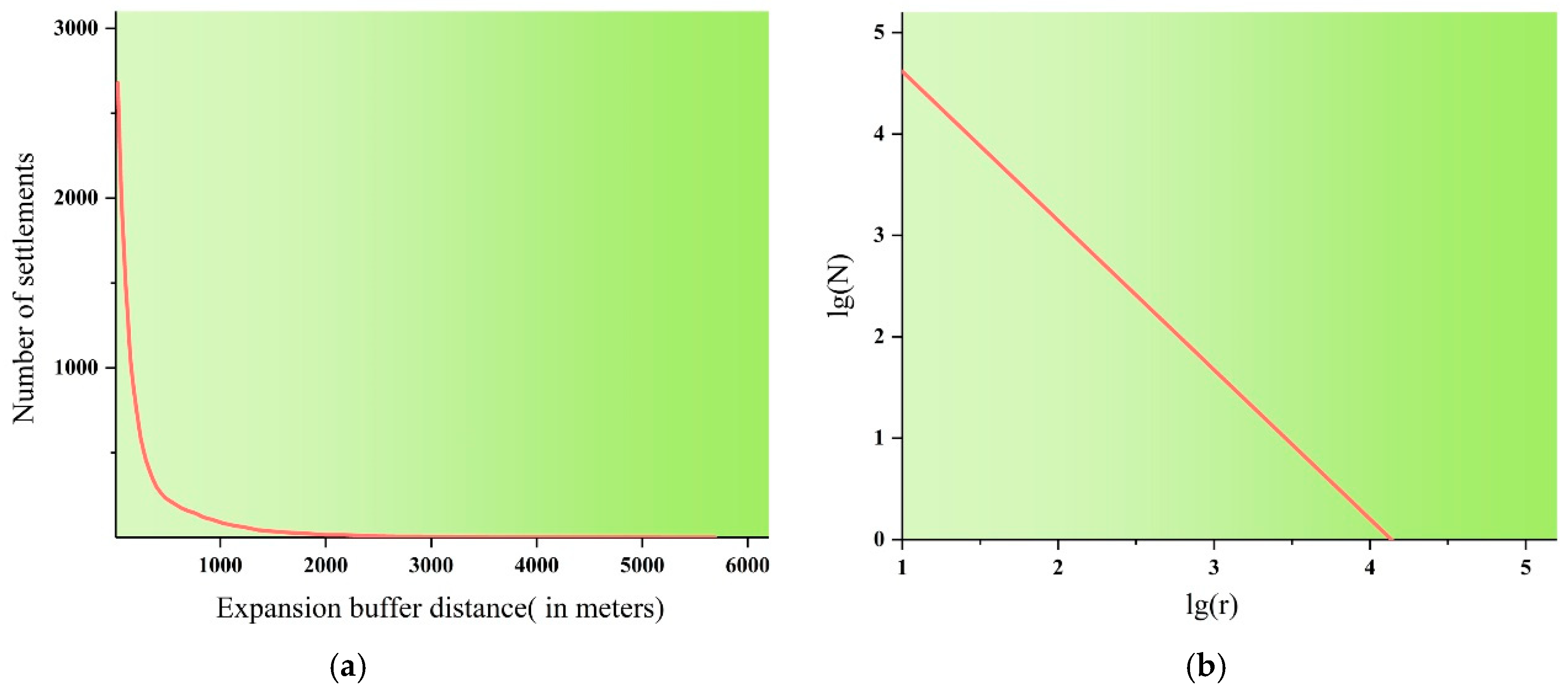
3.1. Urban Expansion Curve

If a city is fractal, the number of its urban settlements is related to the distance threshold, which conforms to a strictly linear relation [63,64]. The true morphology of the city is not a fractal structure strictly following the rules, rather it has random pre-fractal and self-similarity on a limited level [59,65]. The fractal dimension is constant over a limited range, but it changes over a continuous range [66,67]. The power-law relationship between the measurement scale and the corresponding measure is valid only within a certain scale range, thus forming the so-called scaling range [59]. It is assumed that the point deviating from the straight line farthest in the expansion curve is a key distance threshold and corresponds to an urban agglomeration [18] that can separate two spatial forms, namely urban and rural areas. The corresponding principal curvature point can serve as a key point to divide the two spatial form subsets: the urban and rural areas.

The urban expansion curve was constructed under different expansion buffer distances (30 m as the initial expansion buffer distance, and a continuous increase at an equal ratio of 1.1) using the road intersection data set of Guangzhou, Chengdu, Nanjing, and Shijiazhuang, until the map spots merged into a whole. The relationship (based on partial data) between the number of urban settlements and different expansion buffer distances in Guangzhou is shown in

Table 1. Urban expansion of Guangzhou.

Expansion Buffer Distance r/m	Number of Urban Settlements/n	Lg(r)	Lg(N)
30.00	9269	1.48	3.90
33.00	9075	1.52	3.89
36.30	8848	1.56	3.88
39.92	8629	1.60	3.87
43.92	8399	1.64	3.86
48.32	8148	1.68	3.85
53.16	7918	1.73	3.84
58.48	7633	1.77	3.82
64.32	7358	1.81	3.80
70.76	7067	1.85	3.79
77.84	6801	1.89	3.77
85.62	6463	1.93	3.75
94.18	6190	1.97	3.73
103.60	5887	2.02	3.71
113.96	5551	2.06	3.69
125.36	5210	2.10	3.66
137.90	4904	2.14	3.64
151.70	4574	2.18	3.61
166.88	4242	2.22	3.58
183.56	3952	2.26	3.55
202.00	3643	2.31	3.51
222.20	3337	2.35	3.46
244.40	3027	2.39	3.42
268.80	2737	2.43	3.37
295.60	2457	2.47	3.32
325.20	2193	2.51	3.26

. It is obvious that with the increase in the distance threshold, the number of urban settlements generally showed a decreasing trend. With the increase in the distance from 30 to 325.2 m, the number of urban settlements declined from 9269 to 2193, and the urban settlement scale constantly expanded. The selection of an appropriate expansion buffer distance directly affects the identification result of urban settlements. To visually display the change characteristics and differences in the number of urban settlements under different expansion buffer distances in Guangzhou, Chengdu, Nanjing and Shijiazhuang, the expansion buffer distance, and the number of urban settlements in each region were plotted using logarithmic scale mapping as shown in Figure 6. From Figure 6, the changes in the number of urban settlements in the four cities all conformed to the power-law rule, and the shapes of their expansion curves had similarities and differences. The number of initial settlements was the largest in Guangzhou, followed by Chengdu, Nanjing and Shijiazhuang. With the increase in the expansion buffer distance, the number of settlements showed a constantly decreasing trend.

There were three stages in the settlement expansion in the four cities, and the extreme point of curvature could be found in each stage. The expansion buffer distance threshold corresponding to this point could be used to divide the two spatial form subsets: the urban and rural areas. In the first stage, the expansion curve was relatively mild, the number of urban settlements was more than 1000, and the expansion velocity was comparatively slow when the threshold was below 100 m. The expansion buffer distance threshold in Chengdu was the smallest, followed by Shijiazhuang, Guangzhou and Nanjing. In the second stage, the expansion curve was relatively steep, the number of urban settlements was more than 100, and the expansion velocity significantly increased when the threshold was between 100 and 1000 m. The expansion buffer distance threshold from small to large ranked inconsistently compared to the first stage. In the third stage, the expansion curve was steep, and urban settlements gradually merged into a whole when the threshold was above 1000 m. The polynomial fitting times of the four urban expansion curves are shown in

Table 2. Polynomial fitting times and goodness of fit.

City	Polynomial Fitting Times	R2
Guangzhou	8	0.99933
Chengdu	8	0.99904
Nanjing	8	0.99844
Shijiazhuang	8	0.99843

, and the goodness of fit R² was above 0.998 for all cases.

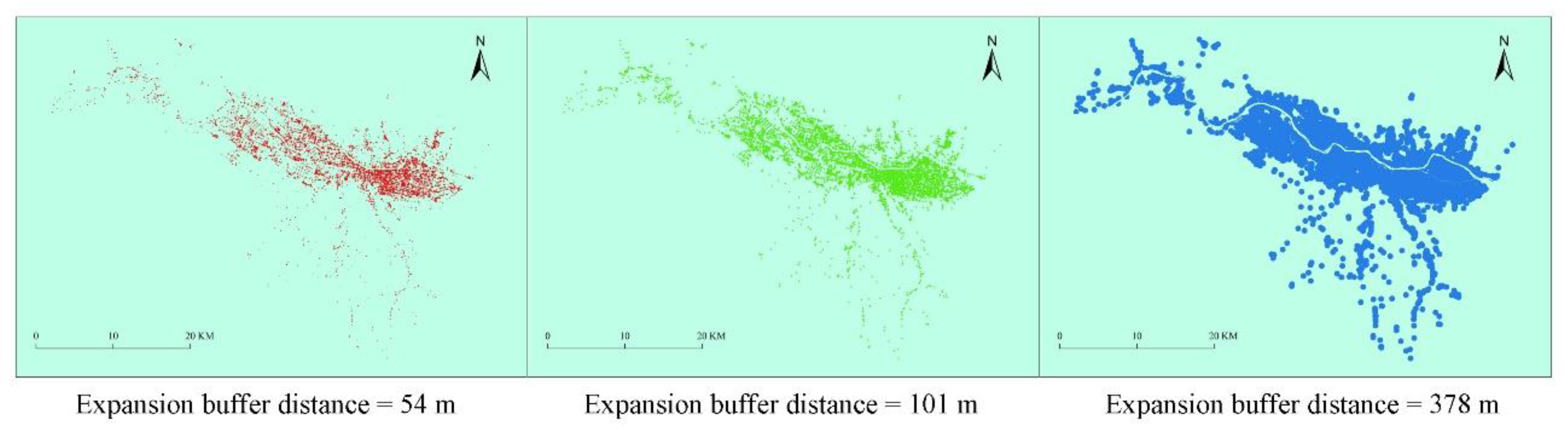
3.2. Identification Results of Urban Settlements

Finding the principal curvature point of the curve is the premise for the urban settlement identification when the urban expansion curve is being considered. Tannier et al. [18,40] opined that for urban boundary identification based on the regional building vector data, the extreme point of curvature with the largest absolute value is the principal curvature point, and the corresponding expansion buffer distance is the key distance threshold [18,61]. As a result, the final identification results can be obtained. Compared with previous studies, there are two distinctions in this paper: (1) This study was based on road intersection data. (2) To reflect on the entire expansion process of urban settlements, no distance interval was defined, and all the data were retained objectively and comprehensively.

The changes in the curvature of the urban expansion curves of Guangzhou, Chengdu, Nanjing and Shijiazhuang are shown in Figure 7. From Figure 7, the curvature changes of the four cities had different shapes and they all had multiple extreme points. If the point with the largest absolute value of curvature was directly selected as the principal curvature point (

Table 3. Curvature extremum of expansion curve.

Guangzhou		Chengdu		Nanjing		Shijiazhuang
Curvature K	Distance Threshold r/m	Curvature K	Distance Threshold r/m	Curvature K	Distance Threshold r/m	Curvature K	Distance Threshold r/m
0.29	60	−1.51	53	0.24	64	0.07	57
−0.99	132	−0.31	104	−0.89	157	−1.01	124
		−0.85	204
−0.12	563	−0.02	821	−0.19	633	−0.37	399
						0.73	5232
						−1.39	8307

), the distance threshold corresponding to the principal curvature point was 132 m, 53 m, 157 m and 8307 m, respectively, and the urban settlement area was 1099.36 km², 190.94 km², 803.07 km² and 5013.36 km², respectively, in Guangzhou, Chengdu, Nanjing, and Shijiazhuang. Compared with the statistical data of the urban built-up area in China Urban Construction Statistical Yearbook 2018, the estimation error rate of the urban area was −15.44%, −79.50%, −1.75% and 1521.82%, respectively, for the four cities. According to

Table 4. Urban settlement area.

City	Distance Threshold r/m	Urban Settlement Area/km2	Built-Up Area/km2	Area Error Rate/%
Guangzhou	60	387.17	1300.01	−70.22
	132	1099.36		−15.44
	563	3776.28		190.48
Chengdu	53	190.94	931.58	−79.50
	104	514.23		−44.80
	204	1076.78		15.59
	821	2738.46		193.96
Nanjing	64	228.19	817.39	−72.08
	157	803.07		−1.75
	633	2880.69		252.43
Shijiazhuang	57	116.56	309.12	−62.29
	124	353.62		14.40
	399	1181.42		282.19
	5232	3917.91		1167.44
	8307	5013.36		1521.82

, the estimated areas of Chengdu and Shijiazhuang were seriously abnormal. In the same vein, the distance thresholds of road intersection were 53 m and 8307 m, respectively, in Chengdu and Shijiazhuang. Note that these results are not consistent with the reality of urban road planning in China. The actual urban size cannot be effectively and accurately reflected simply using the point with the largest absolute value of curvature as the principal curvature point. According to Figure 7, Table 3 and Table 4, when the curvature K value was −0.99, −0.85, −0.89, and −1.01, and the corresponding distance threshold was 132 m, 204 m, 157 m and 124 m, respectively, in Guangzhou, Chengdu, Nanjing and Shijiazhuang, the estimation error rate of urban settlement area was the lowest in Guangzhou and Nanjing. Specifically, the area error rate was −1.75% in Nanjing and −15.44% in Guangzhou, and their estimated areas are slightly smaller than the built-up areas. The area error rate was 14.40% and 15.59% in Shijiazhuang and Chengdu, respectively, and their estimated areas are larger than the built-up areas. Compared with the statistical data of built-up areas, the absolute value of the error rate of the estimated area was within 20% in the four cities. Further analysis also revealed that the distance thresholds corresponding to the above-mentioned curvature points were about 120 m to 200 m. These were all at the curvature extremum with the largest absolute value in the urban expansion curve in the second stage, rather than that in all stages. In this paper, the distance thresholds corresponding to the principal curvature points selected were not found at a few meters or more than 1000 m. This can be attributed to the distance between road intersections. In major cities in China, there are almost no road intersections a few meters apart, or very few ones more than 1000 m apart.

The distribution range of urban settlements in the four cities can be obtained using the key distance threshold (see Figure 8). Guangzhou, located in southern China, is the key city in the Pearl River Delta. The overall urban morphology is mass-shaped, and it shows a fan-shaped expansion pattern. The urban settlements radiate outward from the center of the Pearl River Delta (i.e., the center of Guangzhou) (see Figure 8a). The urbanization rate of surrounding cities is relatively high [68,69]. Due to the centralization and topography of the Pearl River Delta, the urban development leans toward the southwest, and the road intersections in the urban area are dispersed unevenly. There are many large parks and green spaces in the urban area, but the density of road intersections is low. As result, the estimated area error rate is negative. Chengdu, located in southwestern China, is the key city in the Sichuan-Chongqing region. The overall urban morphology is mass-shaped, and the urban settlements display a concentric-circular outward-expansion pattern with old urban districts as the center (see Figure 8b). The urbanization rate of surrounding cities is lower [68,69]. Due to its western development strategy, the urban development leans to the northwest, south, east, and northeast, and the road intersections in the urban area are dispersed unevenly. There are many arable lands interspersed between road intersections in the urban area, so the estimated area error rate is positive. Located in eastern China, Nanjing is the key city in the Yangtze River Delta. The overall urban morphology is band-shaped, and the city develops along both banks of the Yangtze River. The urban settlements on the north bank are loosely distributed in strips and groups, while those on the south bank are densely distributed in strips and clumps (see Figure 8c). The urbanization rate of surrounding cities is higher [68,69]. The road intersections in the urban area are evenly dispersed, and the estimated area error rate is the lowest. Located in northern China, Shijiazhuang is the key city in the Beijing-Tianjin-Hebei region. The overall urban morphology is mass-shaped, and it shows a fan-shaped expansion pattern. A few urban settlements are distributed in the west of Shijiazhuang, while many urban settlements are distributed evenly in the north, east and south (see Figure 8d). The urbanization rate of surrounding cities is lower [68,69]. Due to the Beijing-Tianjin-Hebei integration strategy, the urban development leans to the east, northeast and southeast, and the road intersections in the urban area are dispersed unevenly. There are many arable lands interspersed between road intersections in the urban area, so the estimated area error rate is positive.

In recent years, Chengdu (i.e., the key city of the western development strategy) and Shijiazhuang (i.e., the key city of the Beijing-Tianjin-Hebei integration strategy) have had significant urban development and enhanced urban expansion [70,71]. Under the guidance of government planning (based on the unchanged old urban districts) new urban districts are vigorously developed as functional zones within the administrative boundary of the entire city, but across the district administrative boundary. The distance between the new and old urban districts is relatively large, forming an axis. With advances in the planning and design ideas of the new urban districts, the density of road intersections will be far lower than that in old urban districts, and the corresponding key distance threshold will rise under the impact of new urban districts. This is one of the reasons for having a larger estimated area of urban settlements in comparison to the actual built-up area (i.e., the error rate is positive) in Chengdu and Shijiazhuang.

4. Discussion

Investigating the urban territorial scope is a challenge for both urban geographers and planners [37]. So, if no discussion is made on effective urban territorial scope, the research result will not truly reflect the laws of the development and evolution of the city. At present, nighttime light data and medium- and low-resolution images are used in most cases to identify urban boundaries and the urban territorial scope. However, they rely on spectral features (subject to resolution) and lack spatial details [27,28,72,73]. To a certain extent, using high-resolution images can aid in overcoming these problems by providing more vivid and accurate shape and structural characteristics, to facilitate the extraction of urban boundaries [27].

Zhang et al. used high-resolution images to extract the boundaries of provincial capitals in China in 2000, 2005, 2010, and 2015. However, in terms of practical operation, the identification result cannot be proved repeatedly. This is because it was obtained through automatic identification by computers and manual interpretation and correction [27,28]. In 2010, the administrative region of Beijing only comprised 12 districts such as the Dongcheng District, Xicheng District, and Haidian District (excluding the Pinggu District, Miyun District, Huairou County, and Yanqing County) [27,28]. By magnifying the results of the identification of Beijing’s urban territorial scope in 2010, it can be inferred that a lot of residential areas, streets, and built-up areas were excluded from the urban boundary and the urban territorial scope [27]. The area of the urban territorial scope of Beijing in 2010 was identified as 950–1000 km² [28], which was far smaller than that of its built-up area—1231.30 km², as recorded in China Urban Construction Statistical Yearbook 2011 (note that no data of Beijing can be found in China Urban Construction Statistical Yearbook 2010).

In the urban boundary of Beijing in 2006 (obtained by Tan and Chen by using Landsat remote-sensing images based on the neighborhood dilation quantization method), when the search radius was 45 m, the area of the largest urban settlement cluster was 811.07 km² [26]. The identification results of the area of urban territorial scopes of Guangzhou, Chengdu, Nanjing, and Shijiazhuang in 2015 were 700–720 km², 600–650 km², 450–500 km², and 200–220 km², respectively [28]. In China Urban Construction Statistical Yearbook 2015, the areas of the built-up areas in the four cities were 1237.25 km², 615.71 km², 755.27 km², and 278.05 km², respectively. The areas of the urban territorial scopes of the four cities except Chengdu are all far smaller than the statistics. Chengdu’s area is relatively close to the reported statistics. For the two spatial patterns, cities and rural areas were staggered and discretely distributed at urban boundaries [10,26]. Hence, the identification result of the urban territorial scope was presented as several continuous and closed curves (including enclaves). As a result, the probability of excluding areas from the city area was inevitably increased, leading to smaller areas of identification. Since the definition of an urban boundary is more like the largest urban settlement cluster in the space, it cannot fully and clearly, display the distribution of the whole urban territorial scope in the space [26].

Therefore, it is more scientific to describe urban boundaries based on urban land use classification or fractal thoughts, that is, the urban territorial scope is viewed as discretely distributed urban land or urban settlements [18,29,40]. Data of EULUC-China-2018 (from http://data.ess.tsinghua.edu.cn/, accessed on 1 November 2020) was downloaded, and then ArcGIS was used to work out the data of Guangzhou, Chengdu, Nanjing, and Shijiazhuang, for comparisons with the results of this paper. It can be found that the discrete distribution patterns of the two results in the administrative space of the four cities are almost the same and that their areas of urban territorial scope in the results of EULUC-China are larger (see Figure 9a, Figure 10a–c). The areas of the urban territorial scopes of Guangzhou, Chengdu, Nanjing, and Shijiazhuang in the EULUC-China results are 1985.67 km², 1200.51 km², 1554.74 km², and 776.25 km², respectively. Compared with the data in China Urban Construction Statistical Yearbook 2018 (1300.01 km², 931.58 km², 817.39 km², and 309.12 km², respectively), the error rates of area estimation are 52.74%, 28.87%, 90.21%, and 151.12%, respectively. The areas of the four cities except Chengdu show anomalies.

The b, c, d, e, and f areas of Chengdu in Figure 9a were magnified, and the largest block in the EULUC-Chengdu result of each area was selected. The types of the land for the selected blocks were residential area (5.25 km²), airport facility area (20.97 km²), residential area (5.23 km²), residential area (9.15 km²), and airport facility area (7.20 km²). It can be found that there were several types of land for the selected blocks and that the identification of block boundaries was inaccurate, leading to severely enlarged areas of these blocks. The classification of blocks in the EULUC-China result was also based on the road network of OSM [29]. In an area far away from the city center, the distribution of road intersections became sparse, and, because of the timeliness of OSM data, the distance between road intersections became longer. Therefore, the closer the block is to the urban fringe, the larger its area will be. Moreover, some blocks belonging to other types of land were included, leading to inaccurate identification of block boundaries. Consequently, the identification result of the area of urban territorial scope became enlarged severely.

Urban settlement identification is realized usually through satellite and GIS. Moreover, predefined morphological thresholds are adopted most of the time [14,26,74]. After categorizing basic spatial units, the criterion of contiguity, which usually involves the distance threshold, is applied to group similar units. However, since the two forms of spatial organization, namely the urban area and the rural area, coexist and mix at the boundaries of the cities, showing an irregular pattern, it is difficult to select a single distance threshold [39]. Besides, while analyzing the urban fringe, the selection of the distance threshold becomes a key issue. Therefore, no consensus has been reached currently on the selection of the criterion of contiguity that involves the distance threshold [75]. Urban geographic phenomena have a scale-free property, and the urban morphology and the urban system are fractal. In this paper, with the aid of fractal geometry, predefined distance thresholds were avoided in detecting and measuring cross-scale spatial discontinuity. Instead, multi-scale changes in the established urban morphology were detected and measured to identify urban settlement distribution. Hence, the problem of identifying urban territorial scopes and morphology is adequately addressed. In this paper, based on the fractal urban expansion curve method, the distribution of urban settlements within the administrative regions of Guangzhou, Chengdu, Nanjing, and Shijiazhuang could be quickly identified in an efficient way by using urban road intersection data.

The distance thresholds corresponding to the principal curvature points of Guangzhou, Chengdu, Nanjing, and Shijiazhuang were all below 210 m, and were in the second stage of the urban expansion curve (from 100 to 1000 m). This means that the four cities have fractal features when the distance threshold is comparatively low, indicating comparatively low distance thresholds for the two spatial patterns (i.e., the urban area, and the rural area) within the identification areas. This shares many similarities with the Sierpinski Carpet fractal structure. It is also different from the fractal structure of the spatial organizations in European cities, which is like the Fourier Dusts fractal structure (i.e., the principal curvature point appears at the maximum absolute value of the global curvature extremum) [18,40]. The density of road nodes in the administrative region is generally lower than that of buildings. Therefore, the road intersections of each city will merge in the first stage of the urban expansion curve when the expansion buffer distance is comparatively small. An extremum will appear when the number of nodes sharply goes down and the number of urban settlements increases accordingly. Sometimes, the curvature value in this stage will reach the climax, but it can only reflect the area densely covered by roads in the city. In other words, it cannot truly display urban settlement distribution within the region. In the third stage of the urban expansion curve (above 1000 m), since the number of urban settlements is already very small, an extremum is easy to arise as the expansion buffer distance increases and the urban settlements gradually merge. However, the distance threshold corresponding to the extremum for the time being greatly exceeds the real value as expected. As a result, it cannot be used as a key distance threshold to distinguish between the two spatial forms (i.e., the urban area and the rural area). It also cannot be used to effectively identify the distribution range of urban settlements within the region.

Although the four typical cities are large, the central and core areas are their major development regions, and the fringe areas often receive less attention. This leads to dramatic urban-rural gap in general [76] and a relatively high principal curvature value (between 0.99 and 1.01). Though cities in southern and eastern China are highly urbanized [68,77], it is difficult for them to expand because of huge gaps between urban and rural areas [76], and comparatively low population density. On the contrary, despite a low level of urbanization of the cities in western and northern China, they are prone to expansion because of the relatively small urban-rural gap and high population density. This is different from the research results of Tannier et al. [18,40] in their studies on European cities. For example, in addition to comparatively huge distance thresholds, the three representative cities of Belgium (Namur, Liège, and Charleroi) are highly urbanized, small in the urban-rural gap and high in population density, and they are prone to expansion. As for the three representative cities of France (Besancon, Belfor, and Montbe’liard), they are small in distance threshold and low in urbanization, and have comparatively large urban-rural gaps and low population density, so urban expansion becomes difficult.

Discrepancies to some degree occurred during the estimation of the accurate areas of the four typical cities in China mentioned above. As the central city in eastern China, Nanjing is free of topographical influence due its location on a plain. With the Yangtze River going through the urban area, the urbanization rate of its surrounding cities is higher. Within Nanjing, each district is relatively balanced in development, and the distribution of road intersections along the Yangtze River, is comparatively even. This makes its estimated area to be the most accurate, with an error rate of only −1.75%. Guangzhou is a traditional first-tier city. Due to the influence of urban planning strategies and topography, Guangzhou has shifted its development focus to the center of the Pearl River Delta, resulting in less impact on the key distance threshold. There are many reticular water systems and water areas within the urban area, which reduce the density of road intersections, as well as some large parks and green spaces near those water areas or mountains, so the road intersection density is further reduced accordingly. Though the areas with large parks and green spaces have no urban settlement of certain scale, they have been the urban built-up area. With respect to the fringes of cities, because of the influence of data timeliness and the lack of road intersections, large suburban villages within the city scope were not accurately identified [78]. As a result, the estimated area was smaller than the built-up area in Guangzhou, and the error rate of the estimated area was as high as −15.44%. Besides, Chengdu, an emerging quasi-first-tier city, and Shijiazhuang, a second-tier city, are fast in both economic development and urban expansion. They are also prone to road construction problems. Moreover, during the rapid expansion of the city, a certain number of arable lands have been merged into the city, resulting in the formation of urban settlements in such areas that are not urban built-up areas. Be that as it may, new urban areas rapidly emerge because of the influence of urban planning strategies. Due to the long distance between the new and old urban areas, the key distance threshold is affected to a large extent, ultimately leading to a larger estimated area than the built-up area of the city. Hence, the error rate of the estimated area for the two cities was relatively high, with Chengdu having a rate of 15.29% and Shijiazhuang having a rate of 14.40%.

Conventional methods for urban settlement identification are mostly based on census data [79,80]. Due to the arbitrary designation of the domain of a city in law and administrative measures, not all the people living in the cities are captured by the conventional methods. Holmes and Lee defined a city as a single unit bounded by a 6×6-mile grid and the urban size is measured by the population of settlement within the boundaries of the grid [81]. By clustering the population settlement locations with a predefined distance threshold (for instance 3000 m), Rozenfeld et al. [38] adopted CCA to spot the boundaries of the city. Although these studies seem to have abandoned subjective census data, they relied on population settlement locations. Hence, they designated or defined as urban settlements by census data. In recent years, there has been increasing research on urban boundary identification based on urban building vector data and remote sensing image data, obtaining certain achievements [27,28,29,38,82,83]. For first-tier large cities like Guangzhou, Chengdu, and Nanjing, it is extremely time-consuming to obtain such data. Even if such data was available and successfully interpreted, it is also difficult to ensure the accuracy of attributes and locations. It is well known that human activities are restricted by streets. Without street nodes, there would be no settlement and the resultant formation of a city. Therefore, with improved coverage, the timeliness and accuracy of OSM data and electronic map data, as well as data that can be updated and shared at any time, identification of the urban territorial scope based on road intersections to extract urban settlements may be an effective method. It will not only avoid the subjectivity in basic data, but it will also facilitate the acquisition of the data and improve the quality of the data.

Even though this study can offer a new perspective for the designation of urban territorial scope and the planning of urban system in a region (to further explore the fractal features of cities, use the geographical space and environment more effectively, and to tackle relative urban problems), it is insufficient in some areas. Unlike remote sensing images, the road vector data adopted in this paper fails to reflect the process of urban settlement expansion in the time-domain. The quality of data was affected by the timeliness of road networks in OSM and electronic maps. In other words, the closer the proximity was to city fringes, the worse the identification and updating of road networks became, and some road intersections were missed. Besides, this study only focused on the single urban administrative areas. However, the development of cities has long gone beyond administrative boundaries, to study the sensitivity issue with respect to the cutoff distance thresholds. In the future, it is envisaged that studies will be carried out to explore the urban settlement distribution at a larger spatial scale beyond the administrative areas, such as the Yangtze River Delta, the Pearl River Delta, and even the whole nation. The integration of road networks of OSM and electronic maps with the automatic recognition of high-definition road networks may also become obtainable, to make up the road networks in urban fringes. Moreover, whether the value of the distance threshold has dependence on factors related to topographical water system factors or the spatial form of the city proper requires further investigations.

5. Conclusions

From the perspective of self-organization and based on fractal theory, the following major contributions have been made in this paper (using the adjacency urban expansion curve of road intersections to identify the urban settlement distribution in urban administrative areas):

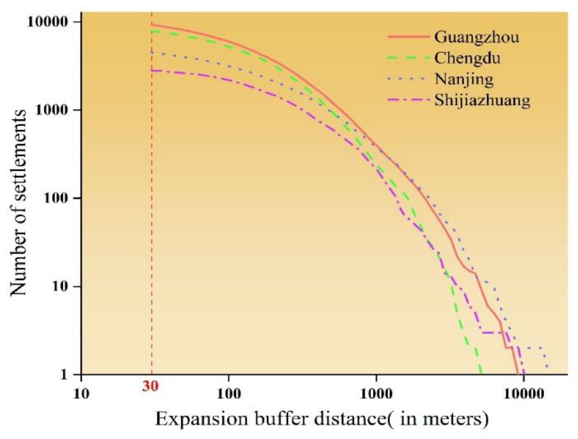
• The research method in this paper is based on road intersection vector data. That is, as the expansion buffer distance increases, the number of urban settlement decreases. Therefore, with the help of fractal geometry, discretely distributed urban settlements and the urban territorial scope of the cities can be obtained through detecting and measuring the multi-scale changes of urban road intersections. This is to find the key distance threshold corresponding to the principal curvature point in the urban expansion curve.
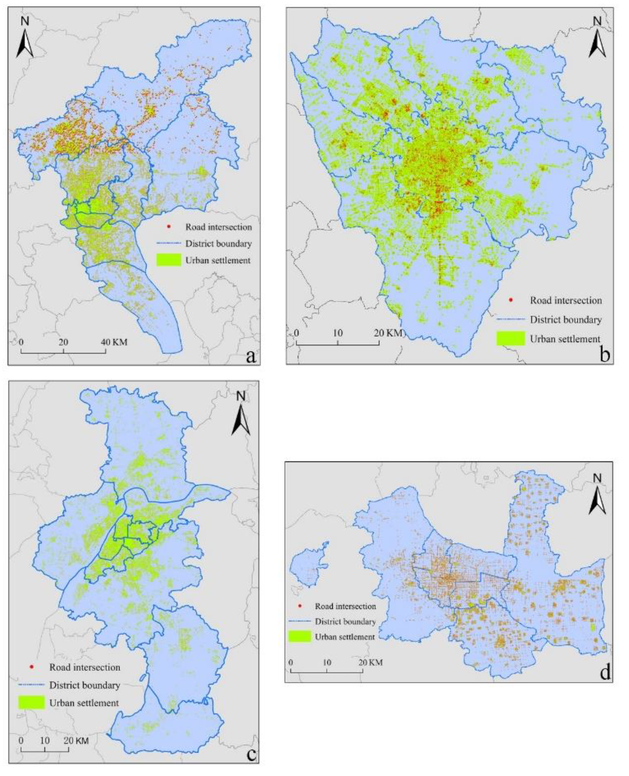
• Among the four representative cities selected for the research, the optimal distance thresholds for the urban settlement distribution in Guangzhou, Chengdu, Nanjing and Shijiazhuang were 132 m, 204 m, 157 m, and 124 m, respectively. This shows that the four cities have fractal features when there is a comparatively low distance threshold (in similarity with the Sierpinski Carpet fractal structure). The areas of urban settlement of the cities corresponding to their optimal distance thresholds were 1099.36 km², 1076.78 km², 803.07 km² and 353.62 km², respectively. These areas are consistent with actual urban built-up areas. This indicates that the method of using road intersections as the data source and using the fractal features of the urban expansion curve to identify urban territorial scope is reasonable and effective.
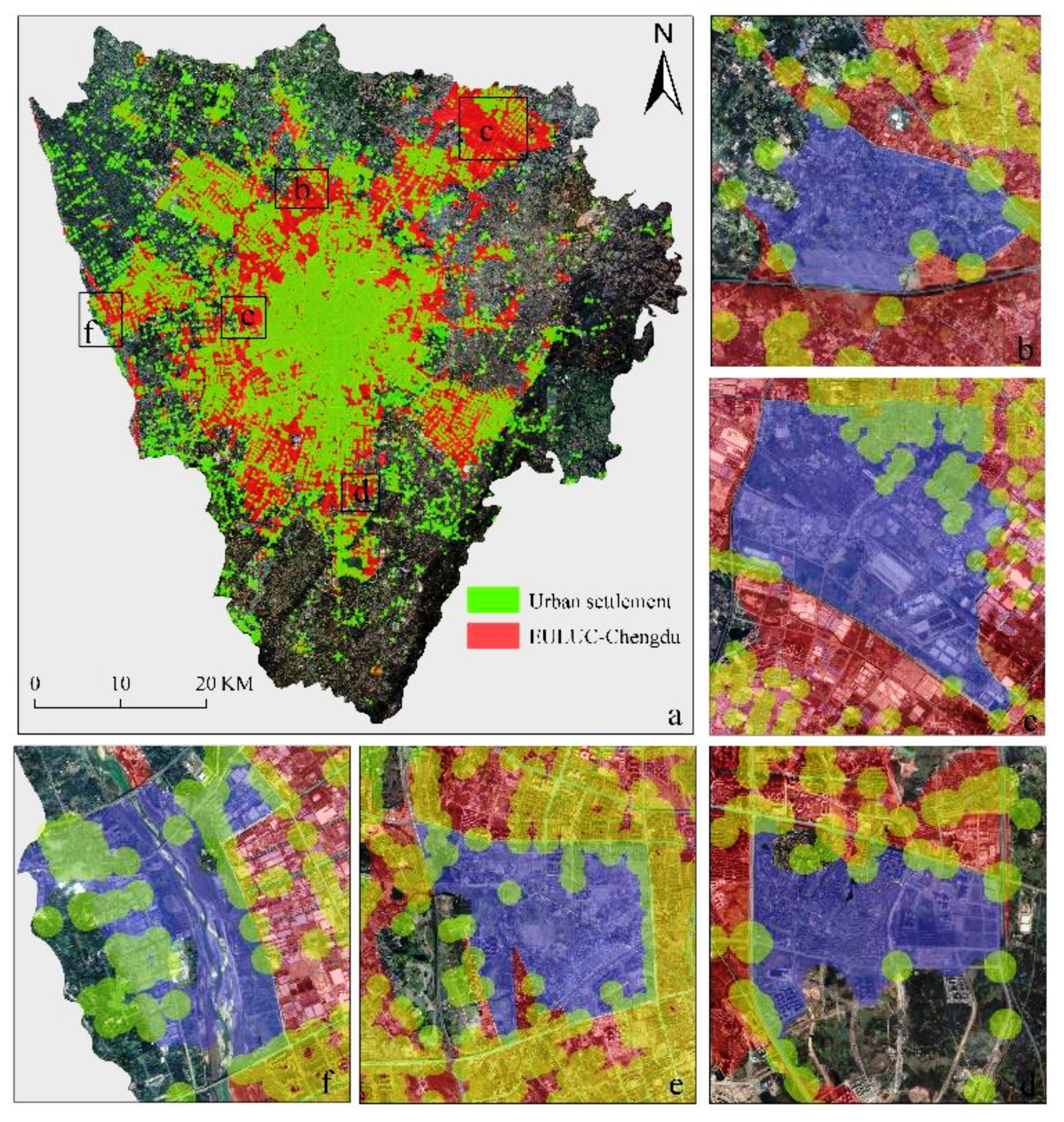
• In this paper, road intersections have been used to extract discretely distributed urban settlements and to identify the urban territorial scope. Because of the influence of large parks, green spaces, or arable land on the fringes of the cities, as well as suburban villages, there is a gap between the obtained area of urban settlement and the actual urban built-up area. Nonetheless, the method in this paper is simple and feasible, and the data adopted are easy to acquire. The results of identification are discrete urban settlements, which are closer, providing free data sources for this study.

References

1. Kuang, W. 70 years of urban expansion across China: Trajectory, pattern, and national policies. Sci. Bull. 2020, 65, 1970–1974. [Google Scholar] [CrossRef]
2. Yue, H.; He, C.; Huang, Q.; Yin, D.; Bryan, B. Stronger policy required to substantially reduce deaths from PM2.5 pollution in China. Nat. Commun. 2020, 11, 1462–1473. [Google Scholar] [CrossRef] [PubMed] [Green Version]
3. Kuang, W. Mapping global impervious surface area and green space within urban environments. Sci. China Earth Sci. 2019, 62, 1591–1606. [Google Scholar] [CrossRef]
4. Kenworthy, J. The Eco-city: Ten Key Transport and Planning Dimensions for Sustainable City Development. Environ. Urban. 2006, 18, 67–85. [Google Scholar] [CrossRef]
5. Li, D.; Liu, L. Context-aware smart city geospatial web service composition. Geomat. Inf. Science Wuhan Univ. 2016, 41, 853–860. [Google Scholar] [CrossRef]
6. He, Q.; Tan, R.; Gao, Y.; Zhang, M.; Xie, P.; Liu, Y. Modeling urban growth boundary based on the evaluation of the extension potential: A case study of Wuhan city in China. Habitat Int. 2018, 72, 57–65. [Google Scholar] [CrossRef]
7. Chaline, C.; Bourne, L.; Simmons, J. Systems of Cities: Readings on Structure, Growth and Policy. Geogr. J. 1979, 145, 489. [Google Scholar] [CrossRef]
8. Chen, Y. Distinguishing three spatial concepts of cities by using the idea from system science. Urban Stud. 2008, 15, 81–84. [Google Scholar]
9. Chen, Y. Fractal Urban Systems: Scaling Symmetry Spatial Complexity; Science Press: Beijing, China, 2008. [Google Scholar]
10. Zhou, Y. Urban Geography; The Commercial Press: Beijing, China, 1995. [Google Scholar]
11. Xu, W. Encyclopedia of China; China Encyclopedia Press: Beijing, China, 2002. [Google Scholar]
12. Standard for Basic Terms of Urban Planning; China Construction Industry Press: Beijing, China, 1999.
13. Levy, M. Gibrat’s Law for (All) Cities. Am. Econ. Rev. 2009, 99, 1672–1675. [Google Scholar] [CrossRef]
14. Jiang, B.; Jia, T. Zipf’s Law for All the Natural Cities in the United States: A Geospatial Perspective. Int. J. Geogr. Inf. Sci. 2010, 25, 1269–1281. [Google Scholar] [CrossRef]
15. Jia, T.; Jiang, B. Measuring Urban Sprawl Based on Massive Street Nodes and the Novel Concept of Natural Cities. 2010. Available online: https://arxiv.org/abs/1010.0541 (accessed on 1 November 2020).
16. Chen, Y. What is the urbanization level of China? City Plan. Rev. 2003, 27, 12–17. [Google Scholar] [CrossRef]
17. Lin, Y.; Hu, X.; Lin, M.; Qiu, R.; Lin, J.; Li, B. Spatial Paradigms in Road Networks and Their Delimitation of Urban Boundaries Based on KDE. ISPRS Int. J. Geo Inf. 2020, 9, 204. [Google Scholar] [CrossRef] [Green Version]
18. Tannier, C.; Thomas, I.; Vuidel, G.; Frankhauser, P. A Fractal Approach to Identifying Urban Boundaries. Geogr. Anal. 2011, 43, 211–227. [Google Scholar] [CrossRef]
19. Chen, Y.; Wang, Y.; Li, X. Fractal dimensions derived from spatial allometric scaling of urban form. Chaos Solitons Fractals 2019, 126, 122–134. [Google Scholar] [CrossRef] [Green Version]
20. Jing, W.; Yang, Y.; Yue, X.; Zhao, X. Mapping urban areas with integration of DMSP/OLS nighttime light and MODIS data using machine learning techniques. Remote Sens. 2015, 7, 12419–12439. [Google Scholar] [CrossRef] [Green Version]
21. Su, Y.X.; Chen, X.; Wang, C.; Zhang, H.; Liao, J.; Ye, Y.; Wang, C. A new method for extracting built-up urban areas using DMSP-OLS nighttime stable lights: A case study in the Pearl River Delta, southern China. GISci. Remote Sens. 2015, 52, 218–238. [Google Scholar] [CrossRef]
22. Zou, J.; Chen, Y.; Ding, G.; Xuan, W. A clustered threshold method for extracting urban built-up area using the DMSP/OLS nighttime light images. Geomat. Inf. Sci. Wuhan Univ. 2016, 41, 196–201. [Google Scholar] [CrossRef]
23. Imhoff, M.L.; Lawrence, W.; Stutzer, D.; Elvidge, C.D. A technique for using composite DMSP/OLS “City Lights” satellite data to map urban area. Remote Sens. Environ. 1997, 61, 361–370. [Google Scholar] [CrossRef]
24. Gibson, J.; Olivia, S.; Boe-Gibson, G. Night Lights in Economics: Sources and Uses. J. Econ. Surv. 2020, 34, 955–980. [Google Scholar] [CrossRef]
25. Yao, J.; Wang, H.; Hu, B. Urban Built-up Area Extraction Based on Vector Data. Bull. Surv. Mapp. 2016, 84–87. [Google Scholar] [CrossRef]
26. Tan, X.; Chen, Y. Urban boundary identification based on neighborhood dilation. Prog. Geogr. 2015, 34, 1259–1265. [Google Scholar] [CrossRef]
27. Zhang, H.; Ning, X.; Shao, Z.; Wang, H. Spatiotemporal Pattern Analysis of China’s Cities Based on High-Resolution Imagery from 2000 to 2015. ISPRS Int. J. Geo Inf. 2019, 8, 241. [Google Scholar] [CrossRef] [Green Version]
28. Wang, H.; Ning, X.; Zhang, H.; Liu, Y. Urban Boundary Extraction and Urban Sprawl Measurement Using High-Resolution Remote Sensing Images: A Case Study of China’s Provincial Capital. ISPRS—Int. Arch. Photogramm. Remote Sens. Spat. Inf. Sci. 2018, XLII-3, 1713–1719. [Google Scholar] [CrossRef] [Green Version]
29. Gong, P.; Chen, B.; Li, X.; Liu, H. Mapping Essential Urban Land Use Categories in China (EULUC-China): Preliminary results for 2018. Sci. Bull. 2020, 65, 182–187. [Google Scholar] [CrossRef] [Green Version]
30. Allen, P. Cities and Regions as Self-Organizing Systems: Models of Complexity; Gordon and Breach: New York, NY, USA, 1997. [Google Scholar]
31. Portugali, J. Self-Organizing Cities. Futures 1997, 29, 353–380. [Google Scholar] [CrossRef]
32. Haken, H.; Portugali, J. A synergetic approach to the self-organization of cities and settlements. Environ. Plan. B Plan. Des. 1995, 22, 35–46. [Google Scholar] [CrossRef]
33. Portugali, J. Self-Organization and the City; Springer: New York, NY, USA, 1999. [Google Scholar]
34. Benguigui, L.; Czamanski, D.; Marinov, M.; Portugali, Y. When and Where Is a City Fractal. Environ. Plan. B Plan. Des. 2000, 27, 507–519. [Google Scholar] [CrossRef] [Green Version]
35. Jiang, B.; Yin, J. Ht-Index for Quantifying the Fractal or Scaling Structure of Geographic Features. Ann. Assoc. Am. Geogr. 2013, 104, 530–540. [Google Scholar] [CrossRef]
36. Jiang, B.; Yin, J.; Liu, Q. Zipf’s Law for All the Natural Cities around the World. Int. J. Geogr. Inf. Sci. 2015, 29, 498–522. [Google Scholar] [CrossRef]
37. Hernán, D.R.; Diego, R.; José, S.A.; Michael, B.H.; Eugene, S.; Hernán, A.M. Laws of population growth. Proc. Natl. Acad. Sci. USA 2008, 105, 18702–18707. [Google Scholar] [CrossRef] [Green Version]
38. Rozenfeld, H.; Rybski, D.; Gabaix, X.; Makse, H.A. The Area and Population of Cities: New Insights from a Different Perspective on Cities. Am. Econ. Rev. 2010, 101, 2205–2225. [Google Scholar] [CrossRef] [Green Version]
39. Chaudhry, O.; Mackaness, W. Automatic Identification of Urban Settlement Boundaries for Multiple Representation Databases. Comput. Environ. Urban Syst. 2008, 32, 95–109. [Google Scholar] [CrossRef]
40. Tannier, C.; Thomas, I. Defining and Characterizing Urban Boundaries: A Fractal Analysis of Theoretical Cities and Belgian Cities. Comput. Environ. Urban Syst. 2013, 41, 234–248. [Google Scholar] [CrossRef]
41. Jiang, B.; Miao, Y. The Evolution of Natural Cities from the Perspective of Location-Based Social Media. Prof. Geogr. 2014, 67, 295–306. [Google Scholar] [CrossRef] [Green Version]
42. Jiang, B. Natural Cities Generated from All Building Locations in America. Data 2019, 4, 59. [Google Scholar] [CrossRef] [Green Version]
43. Whitehand, J.W.R.; Batty, M.; Longley, P. Fractal Cities: A Geometry of Form and Function. Geogr. J. 1996, 162, 113–114. [Google Scholar] [CrossRef]
44. Chen, Y.; Huang, L. Modeling growth curve of fractal dimension of urban form of Beijing. Phys. A Stat. Mech. Appl. 2019, 523, 1038–1056. [Google Scholar] [CrossRef] [Green Version]
45. Frankhauser, P. La Fractalite des Structures Urbaines. FLUX Cah. Sci. Int. Réseaux Territ. 1994, 29, 54–58. [Google Scholar]
46. Makse, H.; Andrade, J., Jr.; Batty, M.; Havlin, S.; Stanley, H.E. Modeling Urban Growth Patterns with Correlated Percolation. Phys. Rev. E 1998, 58, 7054–7062. [Google Scholar] [CrossRef] [Green Version]
47. Makse, H.; Havlin, S.; Stanley, H. Modelling urban growth patterns. Nature 1995, 377, 608–612. [Google Scholar] [CrossRef]
48. Thomas, I.; Frankhauser, P.; Frénay, B.; Verleysen, M. Clustering patterns of urban built-up areas with curves of fractal scaling behavior. Environ. Plan. B Plan. Des. 2010, 37, 942–954. [Google Scholar] [CrossRef]
49. Schneider, A.; Friedl, M.; Potere, D. A new map of global urban extent from MODIS data. Environ. Res. Lett 2009, 4, 44003–44011. [Google Scholar] [CrossRef] [Green Version]
50. Ahmadpoor, N.; Smith, A.; Heath, T. Rethinking legibility in the era of digital mobile maps: An empirical study. J. Urban Des. 2020, 7, 1–23. [Google Scholar] [CrossRef]
51. Jokar Arsanjani, J.; Mooney, P.; Zipf, A.; Helbich, M. OpenStreetMap in GIScience: Experiences, Research, Applications; Springer: Cham, Switzerland, 2015. [Google Scholar] [CrossRef]
52. Huang, X. The Official List of New First Tier Cities in 2019: What’s Your City Rank? Available online: https://www.yicai.com/news/100200192.html (accessed on 1 November 2020).
53. Haklay, M.; Weber, P. OpenStreetMap: User-Generated Street Maps. IEEE Pervasive Comput. 2008, 7, 12–18. [Google Scholar] [CrossRef] [Green Version]
54. Bennett, J. OpenStreetMap Be Your Own Cartographer; Packt Pub: Birmingham, UK, 2010. [Google Scholar]
55. Goodchild, M. Citizens as Sensors: The World of Volunteered Geography. GeoJournal 2007, 69, 211–221. [Google Scholar] [CrossRef] [Green Version]
56. Minkowski, H. Volumen und Oberfläche. Math. Ann. 1903, 57, 447–495. [Google Scholar] [CrossRef] [Green Version]
57. Bouligand, G. Sur la notion d’ordre de mesure d’un ensemble plan. Bull. Sci. Math. 1929, 2, 185–192. [Google Scholar]
58. Goodchild, M. Fractals and the Accuracy of Geographical Measures. J. Int. Assoc. Math. Geol. 1980, 12, 85–98. [Google Scholar] [CrossRef]
59. Chen, Y. Approaches to estimating fractal dimension and identifying fractals of urban form. Prog. Geogr. 2017, 36, 240. [Google Scholar] [CrossRef] [Green Version]
60. Chen, Y. Monofractal, multifractals, and self-affine fractals in urban studies. Prog. Geogr. 2019, 38, 38–49. [Google Scholar] [CrossRef] [Green Version]
61. Lowe, D. Organization of Smooth Image Curves at Multiple Scales. Int. J. Comput. Vis. 1989, 3, 119–130. [Google Scholar] [CrossRef]
62. Schwarz, G. Estimating the Dimension of a Model. Ann. Statist. 1978, 6, 461–464. [Google Scholar] [CrossRef]
63. Chen, Y.; Wang, J. Multifractal Characterization of Urban Form and Growth: The Case of Beijing. Environ. Plan. B Plan. Des. 2013, 40, 884–904. [Google Scholar] [CrossRef]
64. Bettencourt, L.; Lobo, J.; Helbing, D.; Kuhnert, C.; West, G.B. Growth, Innovation, Scaling, and the Pace of Life in Cities. Proc. Natl. Acad. Sci. USA 2007, 104, 7301–7306. [Google Scholar] [CrossRef] [Green Version]
65. Addison, P. Fractals and Chaos: An Illustrated Course; Institute of Physics: Bristol, UK, 1997. [Google Scholar] [CrossRef]
66. Lam, N.; Quattrochi, D. On the Issues of Scale, Resolution, and Fractal Analysis in the Mapping Sciences. Prof. Geogr. 1992, 44, 88–98. [Google Scholar] [CrossRef]
67. Tannier, C.; Pumain, D. Fractals in Urban Geography: A Theoretical Outline and an Empirical Example. Cybergeo 2005, 307, 22–40. [Google Scholar] [CrossRef]
68. Xun, L.; Fan, Y. Problems and development trend of Urbanization. Urban Rural Dev. 2019, 17, 16–21. [Google Scholar]
69. Zong, J.; Lin, Z. 70 Years of Retrospect and Reflection on China’s Urbanization. Econ. Probl. 2019, 9, 1–9. [Google Scholar]
70. Lu, D. Function orientation and coordinating development of subregions within the Jing-Jin-Ji Urban Agglomeration. Prog. Geogr. 2015, 3, 265–270. [Google Scholar]
71. Ren, B.; Zhang, Q. Achievements Experiences and Transition of Economic Development in the Western Region in 20 Years of Development of Western China. J. Shaanxi Norm. Univ. 2019, 4, 46–62. [Google Scholar]
72. Deuskar, C.; Baker, J.; Mason, D. East Asia’s Changing Urban Landscape: Measuring a Decade of Spatial Growth; World Bank Publications: Washington, DC, USA, 2015. [Google Scholar] [CrossRef]
73. World Bank; China Development Research Center of the State Council. China’s Urbanization and Land: A Framework for Reform; World Bank Publications: Washington, DC, USA, 2014. [Google Scholar] [CrossRef]
74. Donnay, J.; Barnsley, M.; Longley, P. Remote Sensing and Urban Analysis; Taylor and Francis: London, UK, 2001. [Google Scholar]
75. Thomas, I.; Frankhauser, P.; Keersmaecker, M. Fractal Dimension versus Density of the Built-up Surfaces in the Periphery of Brussels. Pap. Reg. Sci. 2007, 86, 287–308. [Google Scholar] [CrossRef]
76. Yue, X. Construction of New-Type Urbanization Evaluation System Based on Urban and Rural Coordinated Development. J. Beijing Univ. Posts Telecommun. 2019, 21, 80–90. [Google Scholar]
77. Cai, J.; Zheng, M.; Liu, Y. Measurement and International Comparison of China’s Real Urbanization Level. China Rev. Political Econ. 2019, 10, 95–128. [Google Scholar]
78. Gao, Y.; Shahab, S.; Ahmadpoor, N. Morphology of Urban Villages in China: A Case Study of Dayuan Village in Guangzhou. Urban Sci. 2020, 4, 23. [Google Scholar] [CrossRef]
79. Eeckhout, J. Gibrat’s Law for (All) Cities. Am. Econ. Rev. 2004, 94, 1429–1451. [Google Scholar] [CrossRef] [Green Version]
80. Chen, Y. Scaling Analysis of the Cascade Structure of the Hierarchy of Cities, in Geospatial Analysis and Modelling of Urban Structure and Dynamics; Springer: Berlin, Germany, 2010. [Google Scholar] [CrossRef]
81. Holmes, T.; Lee, S. Cities as Six-by-Six-Mile Squares. Zip’s Law; The University of Chicago: Chicago, IL, USA, 2009. [Google Scholar]
82. Wang, H.; Ning, X.; Zhang, H.; Liu, Y. Urban Expansion Analysis of China’s Prefecture Level City from 2000 to 2016 using High-Precision Urban Boundary. IGARSS 2019—2019 IEEE Int. Geosci. Remote Sens. Symp. 2019, 7514–7517. [Google Scholar] [CrossRef]
83. Zhou, Y.; Tu, M.; Wang, S.; Liu, W. A Novel Approach for Identifying Urban Built-Up Area Boundaries Using High-Resolution Remote-Sensing Data Based on the Scale Effect. ISPRS Int. Geo Inf. 2018, 7, 135. [Google Scholar] [CrossRef] [Green Version]
Figure 1. The study area of Shijiazhuang (a), Nanjing (b), Guangzhou (c), and Chengdu (d).
Ijgi 10 00201 g001
Figure 2. Urban road networks of Guangzhou (a), Chengdu (b), Nanjing (c), and Shijiazhuang (d).
Ijgi 10 00201 g002
Figure 3. Process of the extraction of urban settlements.
Ijgi 10 00201 g003
Figure 4. Schematic diagram of changes in the number of urban settlements.
Ijgi 10 00201 g004
Figure 5. Urban expansion curve (a) and double logarithmic curve (b).
Ijgi 10 00201 g005
Figure 6. Urban expansion curves.
Ijgi 10 00201 g006
Figure 7. Changes in curvature of urban expansion curves of Guangzhou (a), Chengdu (b), Nanjing (c) and Shijiazhuang (d).
Ijgi 10 00201 g007
Figure 8. Urban settlements of Guangzhou (a), Chengdu (b), Nanjing (c), and Shijiazhuang (d).
Ijgi 10 00201 g008
Figure 9. Comparison example for urban territorial scope of Chengdu (a). (bf) are part of the Chengdu.
Ijgi 10 00201 g009
Figure 10. Comparison examples for urban territorial scope of Guangzhou (a), Nanjing (b) and Shijiazhuang (c).
Ijgi 10 00201 g010