Abstract
High-quality digital road maps are essential prerequisites of location-based services and smart city applications. The massive and accessible GPS trajectory data generated by mobile GPS devices provide a new means through which to generate maps. However, due to the low sampling rate and multi-level disparity problems, automatically generating road maps is challenging and the generated maps cannot yet meet commercial requirements. In this paper, we present a GPS trajectory data-based road tracking algorithm, including an active contour-based road centerline refinement algorithm as the necessary post-processing. First, the low-frequency trajectory data were transferred into a density estimation map representing the roads through a kernel density estimator, for a seeding algorithm to automatically generate the initial points of the road-tracking algorithm. Then, we present a template-matching-based road-direction extraction algorithm for the road trackers to conduct simple correction, based on local density information. Last, we present an active contour-based road centerline refinement algorithm, considering both the geometric information of roads and density information. The generated road map was quantitatively evaluated using maps offered by the OpenStreetMap. Compared to other methods, our approach could produce a higher quality map with fewer zig-zag roads, and therefore more accurately represents reality.
1. Introduction
With the development of location-based services, digital road maps are increasingly needed, making road network extraction (RNE) an active research topic. Especially in dense metropolitan cities, people frequently access navigation, route planning, and real-time traffic services, increasing the need for accurate and up-to-date digital road maps. Compared to the time-consuming and labor-intensive conventional map survey, various RNE methods were developed based on remote sensing (RS) images [1,2], GPS trajectory [3,4], and light detection and ranging (LiDAR) point-cloud data [5], since the 1970s. These semi-automatic and automatic algorithms not only lower the cost but also shorten the time of producing and updating road maps. However, due to the inherent drawbacks of the input data, automatically generating high-quality road maps remains challenging [1,3].
Among the existing methods, extracting road networks from RS images is rather mature, and various methods were developed, such as classification-based [6], mathematic morphology [7], road tracking [8,9,10], and active contour [11]. However, these methods are susceptible to the occlusion and shadow in RS images, therefore discontinuous road segments are easy to appear. At present, semi-automatic methods, which require human input, generally perform better than automatic methods.
Road extraction from GPS trajectory data started in 1990; since then, it underwent two stages—map augmentation and map generation. Map augmentation requires an existing map as prior information; conversely, map generation constructs a road map with a topological structure from an empty map. Based on the widely deployed GPS sensors, algorithms can use the collective mobility pattern behind trajectory data to extract semantic information, such as turning restrictions and obtaining GPS trajectory data [12], which is much cheaper compared to RS images or LiDAR data. Given the volume of GPS trajectory data, most of these methods are automatic.
Existing GPS trajectory-based methods can be roughly categorized as follows—clustering-based [13,14,15], kernel density estimation (KDE) [16,17,18], and incremental track insertion [19,20]. These methods face challenges caused by (1) high GPS noise, (2) low frequency, and (3) multi-level disparity problems, which are ubiquitous among easily accessed GPS trajectory data. However, high-quality trajectory data are hard to obtain and covers fewer roads.
To overcome these issues, some methods adopt an intersection-first approach in constructing road maps [14,18]. As intersections are defined as the convergence of three or more road branches, they possess many features that can be detected with a designed algorithm. Detected intersections can serve as valuable information for identifying the road segments connecting them. There has been a recent surge in road intersection detection methods [18,21], which provide a better foundation for this approach. However, few GPS trajectory data-based methods can fully use known intersections, whereas RS-images-based road tracking is mostly driven by points like intersection-centers falling within the region of the road surface.
Therefore, we propose a GPS trajectory data-based road-tracking algorithm, including an active contour-based road centerline refinement algorithm, to extract smoothed and interconnected road centerlines from low-frequency trajectories. By adopting an automatic seeding technique, this map generation method is automatic and thus capable of handling massive trajectory data. The major contributions of our method include.
(1) We enrich the intersection-first approach in extracting road network from GPS trajectory data, making road tracking an available tool to process low-frequency trajectories, which can make better use of known intersections.
(2) We propose a template-matching-based seeding algorithm to automatically provide starting points for the road-tracking algorithm, using the density information of GPS points. To overcome the disparity problem between the heat zone of intersection region and road branches, a circular sampling approach is introduced.
(3) We propose a template-matching-based road direction extraction algorithm to perform correction when tracking road centerlines, which adapts the road-tracking algorithm to GPS trajectory data. To avoid the high GPS noise problem, the real-time correction is simple but robust.
(4) We propose an active contour-based road centerline refinement algorithm to conduct further correction of extracted road centerlines. We include road orientation restrictions in the active contour model to make better use of intersections. The extended post-processing stage makes use of geometric properties of roads, providing a general solution to zig-zag roads.
Our paper is organized as follows. Section 2 reviews the related work on extracting road networks from GPS trajectory data and RS images. Section 3 describes the proposed method for tracking road centerlines. Section 4 presents a set of experimental results and analyses. Finally, Section 5 discusses the conclusions.
2. Related Work
Since the input data are heterogenous, road network extraction methods based on GPS trajectory data are very different from methods based on RS images. Typically, the output road map is represented by a simple graph , where is a set of nodes representing the terminal points of roads, and is a set of edges denoting roads.
First, we introduce the GPS trajectory data-based method. As its input, GPS trajectory data consist of positions of a group of mobile targets across a span of time, sometimes including speed and heading direction. Existing GPS trajectory-based methods can be roughly divided into three categories—(1) clustering-based, (2) KDE, and (3) incremental track insertion.
Clustering-based methods first extract the basic node or edge elements of a road map using a clustering algorithm such as K-means. Then, the road map is constructed by connecting these extracted elements. Edelkamp and Schrödl [13] first extracted a set of seed points spread along the road centerlines, by employing the K-means algorithm to cluster the input GPS points. Then, the adjacent extracted points are connected, based on the connectivity of the trajectories. Karagiorgou [14] first extracted road intersections by employing an agglomerate clustering algorithm to the turn-points, which were defined as where the heading direction changed dramatically. Chen [15] first extracted road segments by employing a graph-based clustering algorithm to a sampling set of input points; then, the intersections were detected by training a support vector machine (SVM) classifier based on their proposed traj-SIFT feature. In conclusion, clustering-based methods generally use the trajectory motion information and therefore suffer more loss from low frequencies.
KDE methods begin with transforming GPS points into a density map through a kernel density estimator, with Gaussian kernel. In most cases, this process occurs in conjunction with discretizing the plane space into the grid of pixels; therefore, image-processing algorithms can be applied to that density map regarding it as a gray-scale image. Biagioni and Eriksson [16] applied an image thinning algorithm on a binarized density map to produce a set of road skeletons using various binary thresholds. These skeletons are merged into a gray-scale skeleton, where an edge’s confidence of being an actual road is represented by its gray scale. Wang [17] proposed a Morse-theory-based road centerlines extraction method, which can capture both heavily- and sparsely-sampled roads with respect to local density. Both methods can produce road maps with different levels of coverage by tuning the parameters and adopting a post-processing approach to better remove the spurious roads. In conclusion, KDE methods are robust to low frequency, but tend to generate zig-zag roads and spurious roads, which requires an effective map refinement algorithm as post-processing.
Incremental track insertion methods construct road maps by incrementally inserting trajectories into an existing map with the help of a map-matching algorithm. Cao and Krumm [18] first grouped similar input trajectories by simulating the physical attraction between them, then incrementally inserted every trajectory by checking whether its node should merge with an existing graph node. Ahmed and Wenk [19] employed Fréchet distance, allowing a trajectory to be partially matched to the map. Different from the first two categories, incremental track insertion methods support online updating, but require high-quality input trajectory data.
Two of the main challenges in extracting road networks from GPS trajectory data are the low frequency and the multi-level disparity of trajectory data; both are ubiquitous among the feasible trajectory data. First, low sampling rate (average sampling interval over 20 s) greatly increases the uncertainty of trajectory data, posing a serious limitation to clustering-based and incremental track insertion methods. Second, the disparity impacts different levels of the extracted road network. At the road level, the staying points of trajectories lead to abnormal local heat zone and distorted road segments. At the network level, the sheer traffic volume difference between different roads makes algorithm tend to mistake roads being travelled by very few trajectories as spurious roads. Finding a global threshold to separate false clusters or roads from correct ones is infeasible.
To address these challenges, researchers are increasingly focusing on the intersection-first approach. Following this approach, road network extraction is divided into two steps—road intersection detection and intersection-based map construction. The difficulty in each step is reduced by adopting a divide-and-conquer strategy. Karagiorgou [14] first proposed a turn-points clustering-based road intersection detection method; Deng [21] introduced a local statistic in clustering-based detection; Zhang [18] proposed a KDE-based detection method, considering the intersection’s heat zone feature. The goal of intersection detection is to achieve both good coverage and precision, under the low-frequency input data.
However, in map construction, most of the existing GPS trajectory-data-based methods only use the intersection’s position; information such as orientations of its connected roads are neglected. Therefore, we combined suitable RS images-based road network extraction methods with this intersection-first approach to more effectively use the known intersections. Here, we focused on briefly introducing the road tracking and active contour methods; both accept a set of seed points as the input, and present roads with a similar parameter model.
Road tracking methods trace the road centerlines by repeating two key steps—prediction and correction. Until a stopping criterion is satisfied, the road tracker traces a single road starting from an initial seed point, which is provided manually or by an automatic seeding algorithm. At the prediction step, an algorithm predicts the next point most likely on the road centerline given the current state of the road tracker. At the correction step, the prediction is corrected by considering its nearby image information, then the state of the road tracker is also updated. Vosselman [8] applied Kalman filter to model the tracking process as a linear dynamic system, and a least squares profile matching was chosen to provide measurement input to the Kalman filter at the correction step. Movaghati [10] combined the extended Kalman filter (EKF) with a particle filter (PF) to find potential new road branches after the road tracker reached its stopping criterion. Road tracking methods are generally sensitive to initial seed points, and face challenge in overcoming intersections, abrupt changes in road direction, and obstructions during the tracing process.
Last, we introduce the active contour method—it defines an energy function on a deformable line, which recursively fits a deformable line to a contour or centerline of a road in the direction of minimal energy, starting from an initialization position. This model was first proposed by Kass [22]; also known as snake, its energy function consists of both internal and image forces. Internal force (elasticity and stiffness) models the geometric features of a road, whereas image force (intensity gradient) represents certain features of interest in the image. Fua and Leclerc [23] proposed the ribbon snakes model to include a width parameter in the image force. By tuning the ratio between internal force and image force, active contour methods can avoid the overfitting problem when extracting roads from an image, which often yields zig-zag roads. As a result, it can also be used as a geometric refinement algorithm for road networks, given background image information.
In conclusion, Figure 1 outlines the rough categories of GPS trajectory-data-based and RS-images-based road network extraction methods. Road tracking methods can also benefit from adopting the intersection-first approach—if intersections and their connected road branches can be detected with high precision and high coverage, the difficulty of road tracking would be significantly reduced. However, due to GPS noise and multi-level disparity problems, the RS images-based methods cannot be directly applied to the density estimation map of GPS points.
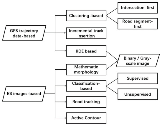
Figure 1.
Road network extraction methods based on two main types of data. RS—remote sensing; KDE—kernel density estimation.
Our method falls into the intersection-first approach category. Based on previous road intersection detection works, we present a combination of KDE and road tracking methods to overcome low-frequency and multi-level disparity of GPS trajectory data in road network extraction. First, we propose a density-based seeding algorithm and a road direction extraction algorithm, both based on template matching, to adapt road tracking to the density estimation map. We adopt a simple real-time correction in this tracking process to avoid tackling drastic GPS noise with limited local information. Then, we apply an active contour-based refinement algorithm to the extracted road network to recursively redo the correction, considering both the geometric information of an entire road and the density information. We emphasize that the impact of disparity is many-fold; by adopting a divide-and-conquer strategy, this problem can be easier solved at the local level.
3. Tracking Road Centerlines from Low-Frequency Trajectory Data
Our road network extraction method starts with a set of known intersection positions, which can be automatically provided by previous road intersection detection works [18,21] or can be input manually. The proposed method consists of three key steps for extracting road centerlines from low-frequency GPS trajectories—(1) generating seed points that exclusively define one end of a road; (2) tracking road centerlines with simple correction; and (3) refining road centerlines based on the active contour model. The workflow of our road centerline tracking method is shown in Figure 2.

Figure 2.
Workflow for extracting road centerlines from GPS trajectories.
3.1. Automatic Seeding Based on Kernel Density Estimation Map
Seed points are the prerequisite of road-tracking algorithms. In our method, a seed point is defined as , where is the start point of road and is the orientation of road at that point (anti-clockwise, equals 0 when heading toward Earth’s true east). Every seed point is derived from an existing intersection, and exclusively defines one end of a road.
Given a known intersection’s center positio , the possibility of having a road branch with orientation is quantitively evaluated by matching the corresponding slice image with a set of ideal road template images. Least squares correlation matching is applied, along with a circular sampling approach, tackling the disparity problem of GPS trajectories. Based on the minimum-matching-distance criterion, multiple seed points can be drawn, and then be examined by the seeding algorithm. Here we use a point-based intersection model, which can cover a majority of intersections with cross-shape, T-shape, and Y-shape.
3.1.1. Density Estimation
Based on the well-known KDE algorithm [24], the sparsely sampled GPS points can be transformed into a consecutive density function on a rectangular domain , which is the area of interest for road network extraction.
Since using a consecutive density function is calculation-intensive, a common practice is discretizing into a grid with a cell-length , and then only computing at the grid center points. Therefore, the density estimation result can be viewed as a gray-scale image , where stands for the density at grid .
Let be the collection of all GPS points. First, a 2D histogram is produced by counting the number of GPS points falling within each grid. Then, the density image is computed as:
where is the popular Gaussian kernel and has a bandwidth parameter . Following a previous work [16], we used .
Notice that . It is faster to compute Equation (1) in two rounds of 1D convolution. Last, we discard the marginal information of , keeping as the central information. These improvements support using a smaller grid cell-length and conducting faster template-matching-based algorithms.
3.1.2. Template Matching
The previous section demonstrated a method to generate global density image from input GPS points. However, due to the GPS noise and the disparity problem [16], automatic seeding requires focusing on the local density image (slice image) to apply pre-processing, such as median filters and image binarization.
Given a position , Figure 3 shows how a slice image with orientation is generated. Let denote the slice image after rotation, for the convenience of matching with a set of fixed road template images. Its pixel value stands for the density at the recalculated grid center , which is computed as:
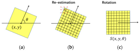
Figure 3.
Generated slice image with arbitrary orientation—(a) the square local area; (b) re-estimating density value on every pixel using the nearby points; and (c) rotating the skewed slice image.
Then, density value is re-estimated using Equation (1) and the nearby GPS points:
where is the Gaussian kernel function. is the image size satisfying m, which means the slice image covers an area of 80 80 m.
Next, we prepare a set of template images based on an ideal road model. A previous work [25] showed that a Gaussian mixture model (GMM) can model the spread of GPS points within a road, reflecting the number of lanes and their corresponding traffic volume in reality. Here, we use single Gaussian model as a simplification, as shown in Figure 4. Therefore, in a road template image, density of one pixel is solely determined by the distance between the pixel center and road centerline.

Figure 4.
Model the spread of GPS points as single Gaussian distribution.
Let denote a road template image with size pixels, its pixel value can be computed as:
where is the orientation of road, and is the bias parameter. The bandwidth was determined by to make the template image cover the entire density descending course. By shifting pixels’ width perpendicular to its road orientation, we obtain . The sizes of the slice image and template image were set to the same value throughout our method.
If the slice image was close enough to a template image, one road was detected in that slice image. When the slice image deviated from the road centerline, the road could still be detected from a broader template set . Since a traffic volume difference might exist between different roads, we could not directly compare pixel value with . Therefore, we applied median filter and binarization to both images as pre-processing, before the matching. Figure 5 shows that the median filter could effectively remove the GPS noise, then the traffic volume was normalized by binarization.
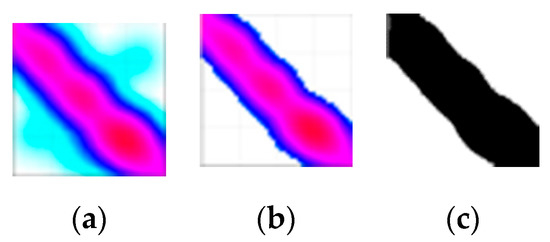
Figure 5.
Pre-processing before matching—(a) the original slice image; (b) after applying the median filter; and (c) after binarization.
Last, the matching should be based on a distance measure between two images. We chose the squared distance for calculation convenience. Given an image , let denote the image after the above pre-processing. The matching distance between two images was defined as:
The smaller the matching distance, the more similar were the two images.
3.1.3. Seeding Based on Template Matching and Circular Sampling
After these preparations, we can now quantitively evaluate the possibility of a road connected to an intersection from arbitrary directions. The search was performed by circular sampling to avoid different road branches, overlapping within the intersection region.
As shown in Figure 6, we categorized the slice image into three classes—(1) road segment, (2) near intersection, and (3) highly noisy area. Experiments showed that the template-matching algorithm worked for road segments and highly noisy areas, but suffered a significant drop in accuracy for the areas near intersections. Detailed experimental results are provided in Section 4.
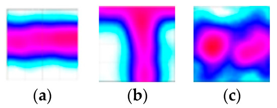
Figure 6.
Three types of slice image—(a) road segment; (b) near intersection; and (c) highly noisy area.
Therefore, we proposed a circular sampling-based seeding algorithm, as shown in Figure 7, to avoid the drawback of the near-intersection areas. Given an intersection’s center position , we used the slice image to detect whether there exists a road branch with orientation . By matching with a set of template images, a matching distance function with the orientation variable was defined as:
where represents how far a deviation we accept from the road centerline; here, we set . Radius was set to 60 m through a series of experiments. Intuitively, smaller represents a higher chance of having a road branch with orientation .

Figure 7.
Detecting road branches based on template matching and circular sampling.
Figure 8 shows that each road branch corresponds to a local minimum of . As a result, by finding all local minimum points of , the corresponding seed points were generated. Since the number of intersections was limited, we adopted a simple enumerating solution in finding these local minimum points. We only computed on a discretized set an angle that satisfied would be selected by our seeding algorithm.

Figure 8.
Matching distance function reflects the possibility of having a road branch with orientation .
However, as shown in Figure 9, the fluctuation of caused by GPS noise led to many false seed points. By applying Gaussian smoothing on , this problem could only be mitigated; therefore, we proposed density-based connectivity to verify the generated seed points. Given two planar points , let denote the connectivity between these points.
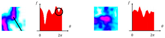
Figure 9.
Fluctuation in matching distance function results in false road branches.
The proposed connectivity ranged from 0 to 1. Assuming is the intersection’s center position, when refers to a false road branch, the density value drops quickly along , which results in low connectivity. Figure 10 shows that true road branches tend to have larger integral area under curve , therefore, a connectivity threshold can effectively separate the false road branches from the true ones.

Figure 10.
Linearly sampled density value along a road branch’s orientation.
Figure 10 also shows that, in most cases, the start point has a much higher density value for traffic from different road branches overlapping at the intersection, which results in a lower in general. Therefore, when verifying a seed point by computing density-based connectivity, the segment falling within the intersection region should be truncated, as follows:
where and is a predefined connectivity threshold. We set through a series of experiments. The other two parameters m and m were set through visualization, as shown in Figure 11. Seed points that satisfied Equation (8) were considered true, and were fed to the road-tracking algorithm in the next step.
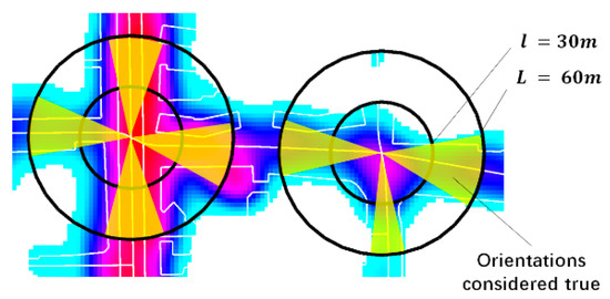
Figure 11.
Seed points with drastic density change from inner circle to outer circle are considered false.
3.2. Tracking Road Centerlines Based on Kernel Density Estimation Map
After the seeding algorithm generated a set of seed points from the density map, the tracking algorithm set up multiple road trackers to incrementally generate estimation curves of road centerlines. Each tracker corresponded to a single seed point . The estimation curves were further refined in the next post-processing course.
Here, we used a simple graph to model the output road network, with known intersections as its initial vertex set . For every road tracker, the prediction and correction two-step process was repeated—at the prediction step, the algorithm calculated the position of a new vertex based on the current state of the road tracker (using a predefined road model), and the successive positions formed the edges of the graph . At the correction step, the algorithm measured the local density map around the newest position to refine the prediction and update the current state of the road tracker. As such, new edges were incrementally added to the shared graph , until a stopping criterion was satisfied. Figure 12 shows the flow chart of our road-tracking algorithm.

Figure 12.
Flow chart of the road-tracking algorithm.
3.2.1. Road Model
We first introduced a road model that was used by previous methods [10], which models one road as a series of states . Here, attribute represented the orientation of the road at position , represented the curvature of road at , and formed a polyline representing the road centerline. Figure 13 shows that this definition of road state contained the necessary information to predict the most likely next point on the road centerline, along with other crucial road attributes.

Figure 13.
Road model.
Previous methods also modeled the tracking process as a stochastic process [8,10]. As a result, the prediction step could be written in an equation form:
where is the tracking step length parameter and represents the random variation in the road state between successive positions. The next step was measuring the local density map to support the correction step, which is referred to as another equation called the measurement equation:
where represents the measurement noise. Assuming that both Equations (9) and (10) were linear and both and were Gaussian noise, the classical correction based on the Kalman filter could be derived [8].
However, since precisely modeling and was infeasible for GPS trajectory data under complex urban environments, we adopted a simple correction in the tracking process by replacing and with a zero matrix. The underlying assumption was that roads have a fixed curvature except for a few turn-points.
3.2.2. Road Orientation Extraction Based on Template Matching
To support the correction step, we measured two attributes from the local density map of the predicted state , based on the template matching previously introduced in Section 3.1.2. Attribute represented the road orientation at the predicted point , and represented the grid deviation from the road centerline at a predicted point.
Since the tracking process required excessive measurements, we introduced another matching mode requiring far less computation. Recall that in Section 3.1.3, generating a slice image by redoing the density estimation placed a heavy computation burden on the seeding algorithm. Therefore, in this section, we only computed a slice image with fixed , and let denote the enlarged template image set, based on discretized orientations:
Using the same minimum-matching-distance criterion, the measurement result was obtained as:
where belonged to the pre-generated set . Here, we used ° and , which could satisfy the simple correction needed.
Figure 14 demonstrates the difference between the two matching modes. By allowing the slice image to have an arbitrary orientation, the algorithm could use more local density information, but the computation cost was not equivalent to the gain.
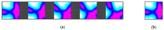
Figure 14.
Difference between two template-matching modes—(a) slice images with variable orientation allow for using more image information; and (b) fixed slice image is less computationally intensive.
3.2.3. Road Tracking Algorithm
In this section, we combined the road model and the measuring algorithm to present our road-tracking algorithm. Starting with the density map and a set of seed points, this algorithm incrementally built a road network with a topological structure. The tracking algorithm consisted of the following five steps:
(1) Initialization: For every seed point , create a road tracker with an initial state , and let distinguished seed positions be the initial vertex set of road network .
(2) Prediction: For every road tracker, based on the current state and Equation (9), compute the predicted state .
(3) Measurement: Based on the predicted state and Equation (12), obtain measurement result and from density map .
(4) Correction: Based on the measurement result and the following equation, compute the corrected state :
where is the grid cell length and is the tracking step length.
(5) Stopping Criterion: Based on the current state and corrected state examine two stopping criteria with their positions and . First, examine the absorbing criterion using the extracted road network and the tracking step length:
If Equation (14) is satisfied, then is absorbed by the closer vertex or of the road network, and a new edge from to the absorb-vertex is added to the road network. Then, the corresponding road tracker stops. Otherwise, examine the density-connectivity criterion using Equation (7).
where is the same connectivity threshold in Equation (8). If Equation (15) is satisfied, it is likely that the newly extracted road segment crossed a road edge or ran into a dead end (zero density area). The corresponding road tracker stopped and the new edge was nullified in this situation. Otherwise, a new vertex and edge were added to the road network, and the road tracker continued tracking with the newest state , by repeating steps (2) to (5).
The tracking step length played a key role in our road-tracking algorithm. Intuitively, when the step length was too large, the road tracker could not handle the dramatic change in road orientation well. Conversely, when the step length was too small, the road tracker would be trapped or distorted by the local heat zone of the density maps, such as the intersection regions. Here, we chose m through a series of experiments.
As shown in Figure 15, after the input of ground-truth intersections, our road-tracking algorithm could generate continuous road centerlines interconnected to form a network, and achieved good coverage of existing roads (travelled by at least three trajectories). This provided a solid foundation for post-processing, to further enhance the quality of the road network.

Figure 15.
The result of road tracking using the Shenzhen taxi trajectory data—(a) comparison with the complete map available online (extracted roads are marked with thick lines, thin lines stand for roads from OpenStreetMap, which are well overlapped with the color map offered by BaiduMap, and the Chinese labels stand for street name); and (b) coverage on roads travelled by at least three trajectories (green line means covered).
In conclusion, the proposed template-matching-based road-orientation-extraction algorithm adapted the road-tracking algorithm for the GPS trajectory data. Although the correction step was simple, it considered 80 80 m area of local density information and was robust enough. A road-intersection-detection algorithm with high recall could help the road-tracking algorithm to avoid tackling the challenging intersection regions in advance.
3.3. Road Centerline Refinement Based on Active Contour
Due to the high GPS noise, most existing KDE-based road-network-extraction methods produced a number of zig-zag roads in the extraction result, as shown in Figure 16. The proposed road tracking algorithm faced the same problem—due to the discretized output of the measurement algorithm, the extracted road centerlines often have fluctuating orientations on consecutive points, resulting in zig-zag roads, especially when the tracking step length is small.

Figure 16.
Orientation restrictions cause non-straight road to also be the optimization result (assuming that the image force equals to zero).
Developing a density-aware road-centerline-refinement algorithm provided a general solution to this problem. We chose an active contour model for it defined an energy function on a deformable line, including a pair of structural internal force and external image force; therefore, it could balance between generating straight roads and over-fitting zig-zag roads. The refinement algorithm took a road centerline from a road-tracking algorithm as its input; based on a predefined energy function, the geometric refinement of the road centerline was done by minimizing its energy, yielding a smoothed road.
3.3.1. Active Contour Model
In this section, we introduce the definition of the original active contour model by Kass [22], along with the minimization procedure, through variational calculus. Let denote a deformable line in plane space, its energy function is defined as:
where represents the internal energy, which controls the shape of curve with its first-order term and second-order term; represents the image energy when is placed on a background image. Parameter is also known as the elasticity parameter, where setting a larger results in an optimal curve closer to the shortest path; and parameter is also known as the stiffness parameter, where setting a smaller allows the optimal curve to have a more drastic change in direction.
Based on Equation (16), the optimal curve was defined and obtained by minimizing the total energy. Kass proposed a numerical method using the Euler–Lagrange differential equation. If curve extremized the functional , then the following equation was satisfied:
Turning Equation (16) into discrete form yields an easier solution method, especially when and were not constant. Following Kass’ approach, two independent Euler–Lagrange equations could be drawn from Equation (17), and could be written in matrix form as:
where and represent the coordinates of nodes in the curve. is a sparse coefficient matrix composed of and at these nodes. = and = are the derivatives of the image force.
Solving from Equation (18) yields the optimal curve, which could be achieved by recursively computing the following equations, starting from the initial curve :
where is a step parameter and is an identity matrix. The inverse matrix of could be computed by decomposition. When the total energy change was less than a threshold, the curve converged to a local minima.
3.3.2. Geometric Refinement of the Extracted Road Centerlines
Based on the active contour model, the geometric refinement of a road centerline could be defined as minimizing its energy, yielding a smoothed road. The refinement algorithm took its input from the road-tracking algorithm.
To solve the optimal road centerlines, first, we computed the coefficient matrix . In our case, curve was unclosed and had two fixed ends, resulting in the boundary conditions and . As and were fixed, we could only optimize the remaining points; therefore, was an pentadiagonal banded matrix:
where by Kass’ approach [22].
Following the common assumption made by road-tracking methods that road centerlines generally have low curvatures, we could assume that and were constant, except for a few turn-points. If is a turn-point, then is set to 0, and the th row of equals . The adaptive selection of turn-points is discussed later.
Next, we introduced orientation restrictions and to consider road orientations at both ends, as shown in Figure 16. We included orientation restrictions in a matrix form into Equation (18). Here was satisfied, as we want orientation restrictions to only directly affect the first points of a road from two ends.
To determine , since orientation restrictions were independent from image information (we could assume that the image force equaled to zero), the following equation held true for the optimization result:
Focusing on one side of the road, one could make a reasonable assumption that also held true, where was defined by prolonging the road in the opposite orientation. Based on these assumptions, and could now be solved using the first two rows of coefficient matrix :
where was computed by using the road orientation and tracking step length. By similarly computing and , yielded the complete restriction matrix .
Previous works demonstrated that road centerlines could be viewed as mountain ridges of the density field [17]; therefore, we define the image force as a negative density value . However, due to the disparity problem, the image force varied largely from curve to curve, making it infeasible to apply a set of global parameters. Therefore, the image force must be normalized at the local level. Combining the orientation restrictions, Equation (18) was rewritten as:
where is the normalization factor, which was computed using the density value along the curve . The new equation could still be solved by Kass’ approach (see Equation (19)).
Last, we identified four tuning strategies through a series of experiments:
(1) Set a rather small ; therefore, the image force plays a priority role in refining road centerlines;
(2) Set a rather large ; here, we use ;
(3) Set a rather large step parameter ; here, we use ;
(4) Allow the curve to have multiple adaptively selected turn-points, where is satisfied.
We briefly introduced these strategies. Since the input curve from the road-tracking algorithm was close enough to the real road centerline, a large step parameter could produce a robust iteration course. The impact of disparity was multi-level; local heat zones existed in the road due to the stay-points in the trajectories. Figure 17 shows that these heat zones might distort an active contour, as the image force dragged its points into a density peak. Setting a larger could mitigate this problem; however, it produced a new problem—if and were constant, the active contour could not accurately fit a road with drastic changes in orientation (Figure 18a).
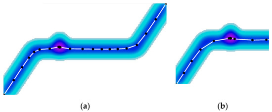
Figure 17.
Geometric refinement result—(a) smooth in general; and (b) distorted by local heat zone.
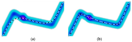
Figure 18.
Fitting a road with drastic changes in orientation—(a) considering no turn-points; and (b) allowing adaptive selection of turn-points.
A previous work [11] showed that introducing turn-points could solve this problem (Figure 18b). At a turn-point, was set to 0, allowing the optimal curve to drastically change in orientation. Turn-points could be adaptively selected by checking whether the orientation change in the initial curve was larger than a given threshold (e.g., ). Experiments showed that the adaptive turn-points could considerably improve the geometric refinement of road centerlines, which significantly reduced the zig-zag roads in the extracted road network.
4. Experimental Results
4.1. Datasets and Evaluation of the Extracted Road Network
Real trajectory data of taxis in the Shenzhen city [12] were used to verify the effectiveness of our road network extraction method using low-frequency GPS trajectory data. The Shenzhen dataset contained over 75 million GPS points from 14,716 taxis, with an average sample rate of 26.1 s [26], collected in one day, which represented feasible but low-quality GPS trajectory data. In our experiments, only a subset covering an area of 2.0 2.0 km was used for quantitative evaluation (Figure 19). The ground-truth map was provided by OpenStreetMap (OSM) [27], and we only kept roads that were travelled by at least three trajectories. The partial Shenzhen taxi trajectory data and manually processed OpenStreetMap can be found in supplementary material.
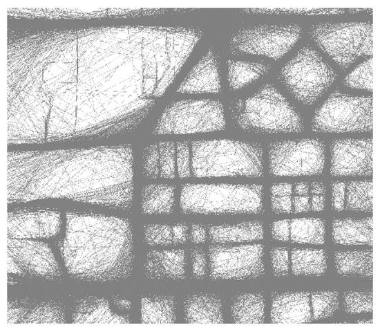
Figure 19.
Raw GPS trajectories collected by taxis in Shenzhen (partial).
To compare the extracted road network with ground-truth data, we adopted a graph-sampling-based distance measure proposed by Biagioni and Erikson [3]. This measure considered both the geometric and topological similarity of maps. The sample points on the extracted road network were called marbles, and the sample points on the ground-truth road network were called holes. If a marble was close enough to a hole (judging from a predefined distance threshold), a matched marble and a matched hole were yielded. Based on this intuition, two metrics could be computed by counting the matched marbles and holes: (1) and (2) . Combing these two metrics, the F-score could be computed as:
where and .
The F-score represents the proximity of the extracted road network to the ground-truth map, under a specific distance threshold. Changing the distance threshold could reflect different standards for evaluating a generated road network, from satisfying commercial requirements to visualization needs. In our experiments, a set of distance thresholds was used.
4.2. Evaluating Extracted Road Network
4.2.1. Parameter Tuning
Our method consisted of three steps—automatic seeding, road tracking, and road centerline refinement. The tracking algorithm was sensitive to the generated seed points, therefore automatic seeding is a key step, which involves two critical parameters—the circular sampling radius and the density-connectivity threshold .
The parameter tuning was based on the ground-truth intersections offered by OpenStreetMap. The generated seed points were evaluated by computing the error of road orientation using known road branches of the ground-truth intersections. Using a fixed degree threshold °, Table 1 shows the precision and recall of the generated seed points (before density connectivity check), using different circular sampling radius

Table 1.
Comparison of generated seed points before connectivity check.
It could be seen that as sampling radius increased, the number of generated seed points increased, however, the recall first increased and then decreased. Both precision and recall reached its maximum value when was 60 m. Based on this parameter setting and a loosened degree threshold of 15°, Table 2 shows the precision and recall after the density-connectivity check, using different threshold
Table 2.
Comparison of the generated seed points after connectivity check.
The density-connectivity check tried to remove the false seed points without misclassifying the true ones. About 5.2% of the generated seed points could not match with any ground-truth seed points, even when the degree threshold was greatly loosened. In this case, a connectivity threshold of 0.1 was able to remove half of the false seed points, while preventing the recall from decreasing too much.
The proposed road-tracking algorithm involved one key parameter, the tracking step length . Since the road centerlines would be further refined in post-processing, here, we focus on the recall and complexity of the road network generated by road tracking. We use ground-truth seed points as input to exclude road tracking’s sensitivity to seed points. The distance threshold in evaluation of the road network was set to , causing every extracted road be counted in the recall.
As shown in Table 3, given the correct seed points, the proposed road-tracking algorithm showed the robustness for covering the existing roads. Either too small or too large led to redundant vertexes and edges, resulting in more spurious roads. Lastly, Table 4 lists the parameter settings for full experiments.
Table 3.
Comparison of the extracted road network before the road centerline refinement.
Table 4.
Parameter settings for experiments.
4.2.2. Evaluation of the Extracted Road Network
Since previous intersection detection methods [18,21] lacked a positioning error evaluation of the detection result, the first part of our experiments was based on the ground-truth intersections. The simulation result using intersections with different coverages and noise levels is discussed in the next section.
Table 5 shows that our method achieved both relatively high precision and high recall when extracting road networks, if the input intersection was high quality. In the recent road intersection detection method proposed by Deng [21], a high precision (94.52%) was achieved using low-frequency trajectory data in Wuhan, but the recall (55.65%) was rather low. Intuitively, a recall-focus intersection detection method could better meet our method’s needs to cover more roads in the extraction result.
Table 5.
Comparison of the extracted road networks.
Table 5 also shows that the quality of automatically generated road network was still inadequate for commercial applications such as navigation and automated driving, a more realistic usage could be identifying changes and missing roads in the existing map, at a daily level (noticed that the Shenzhen dataset we used was collected on one day).
Figure 20a shows that our method could generate smooth road centerlines from the noisy and unevenly distributed density map. Figure 20b demonstrates the performance of geometric refinement, which shows that the refined roads achieved a balance between straight road and zig-zag roads, connecting the local peaks of the density field. However, the refined road was still susceptible to the heat zone of intersection region near its two ends.

Figure 20.
Effectiveness of active contour-based road centerline refinement—(a) the smoothed road centerlines; and (b) comparison of tracked roads and refined roads.
In conclusion, quantitative evaluation and visual inspection demonstrated our method’s effectiveness as a semi-automatic method, the automatic one would continuously benefit from the development of the road-intersection-detection method. However, the position of intersections was not refined by our method. There were also a small proportion of spurious roads in the extracted road network, derived from the false seed points, which required a more in-depth research on an active contour-based road network refinement.
4.3. Analysis
4.3.1. Analysis of Template Matching
To verify the template-matching algorithm, we randomly sampled 176 slice images of a road with ground-truth orientation offered by OpenStreetMap, and then manually labeled them as road segments (total of 111 slices), near intersection (total of 40 slices), or highly noisy area (total of 25 slices). Figure 21 shows that based on the minimum-matching-distance criterion, our orientation extraction algorithm worked for the dominant road segment area; therefore, it could satisfy the need for simple correction of the road-tracking algorithm. Figure 21 also shows that adopting a circular sampling approach in the automatic seeding algorithm was crucial to preventing the areas near intersections from undermining the matching distance function.

Figure 21.
Experimenting road orientation extraction algorithm for three types of slice images.
4.3.2. Analysis of Automatic Seeding
First, we verified the effectiveness of density connectivity check using ground-truth intersections as input. Figure 22a shows the statistical result of matching the generated seed points with ground-truth road branches, from which we observed a proportion of obvious false seed points having an unacceptable orientation error (60°). Figure 22b shows that after the density connectivity check, these obvious false seed points were removed, increasing the precision of the generated seed points at a small cost of recall.
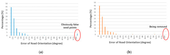
Figure 22.
Error when determining the road orientation of seed points—(a) before and (b) after density connectivity check.
Table 6 lists the detail precision, recall, and the F-score of the generated seed points (after density connectivity check), using different degree thresholds. As shown in Table 6, our seeding algorithm could balance precision and recall.
Table 6.
Evaluation of generated seed points.
Next, we analyzed the sensitivity to input intersection positions under the fixed degree threshold of 7.5°. Since the previous road-intersection-detection methods lacked the fundamental positioning error model, we modeled the positioning error as 2D Gaussian distribution, and introduced circular error probable (CEP) to represent the noise level. When the CEP was meters, 50% of the positioning error were within meters. Figure 23 shows that the highly noisy intersection input eventually lowered the performance of the seeding algorithm, posing a moderate requirement on the precision of the road intersection detection method.

Figure 23.
Evaluation of the generated seed points under different noise levels. CEP—circular error probable.
4.3.3. Input Sensitivity Analysis
Last, we tested the stability of our road network extraction method using simulation intersections with different coverages and noise levels (CEP). We modeled three types of input intersection—(1) ground-truth, (2) precision-focused, and (3) recall-focused. Simulation intersections were generated by randomly picking from ground-truth intersections and then adding 2D Gaussian noise to the center position; the detail CEP and recalls of different inputs are listed in Table 7.
Table 7.
Three types of input intersections.
The ground-truth input represents the manually selected input, provided by human operators or OpenStreetMap. The precision-focused input represents previous precision-focused road intersection detection methods; here, the recall was determined from the recent work by Deng [21]. The recall-focused input represents ideal methods that could better meet our method’s need.
As shown in Figure 24, using the precision-focused input, our method could more accurately generate parts of the road network. However, it would eventually miss about 20% of the existing roads. Using recall-focused input, this automatic approach could cover over 90% of the existing roads in the extraction result, regardless of the moderate intersection position error. Its ability to cover existing roads was very close to the semi-automatic approach. Finally, if the vertex of extracted road network could also be refined, which was what our method lacked, the map quality could be further improved.
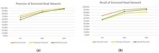
Figure 24.
Comparison between three types of input intersections—(a) precision; and (b) recall.
5. Conclusions
In this paper, a low-frequency GPS trajectory data-based road network extraction method was proposed. The feasibility of GPS trajectory data provided a new means to automatically generating road maps. However, the prevalence of low sampling rate and multi-level disparity complicated the achievement of both high precision and high coverage in the generated map. Among various road-network-extraction methods, the intersection-first approach used the valuable information from road intersections in a divide-and-conquer manner, and it could be further benefited from the development of intersection-detection methods. Therefore, we followed this approach to propose a combined method that applied a road-tracking algorithm on the density map estimated by the KDE algorithm, where information of road intersections was represented as automatically generated seed points.
We found that the divide-and-conquer strategy was the key to tackling the multi-level disparity problem. By ruling out the near intersection region in advance, the template matching-based road-orientation-extraction algorithm performed better in general. The road-tracking algorithm could trace a road connecting two known intersections with more robustness. We pointed out that a recall-focus road-intersection-detection method could better suffice the need of road network extraction in this approach. By adopting an active contour-based road-centerline-refinement algorithm, our method yielded smoothed road centerlines than the traditional KDE-based methods. Compared to the previous GPS-trajectory-data-based road-network extraction methods, our method achieved a good balance between precision and recall using low-frequency trajectories. Moreover, the proposed road centerline refinement algorithm could serve as a general solution to zig-zag roads, considering both road structure and image information.
However, our method lacks the ability to refine the position of road intersections and to handle complicated intersection structures (e.g., highways and roundabouts). There also exists a small proportion of spurious roads due to false seed points, which requires an in-depth road-network-refinement method. Therefore, our future work will focus on applying the active contour for optimizing the position of a known intersection, and developing its ability to extract the precise boundary of city blocks from a density map, which is helpful in identifying the dead-end roads.
Supplementary Materials
The following are available online at https://www.mdpi.com/2220-9964/10/3/122/s1, the partial Shenzhen taxi trajectory data and OpenStreetMap we used in experiment is added in the supplementary file.
Author Contributions
Conceptualization, Banqiao Chen, Chibiao Ding, and Wenjuan Ren; Methodology, Banqiao Chen, and Chibiao Ding; Software, Banqiao Chen; Validation, Banqiao Chen; Formal Analysis, Banqiao Chen; Investigation, Banqiao Chen; Resources, Guangluan Xu; Data Curation, Banqiao Chen; Writing—Original Draft Preparation, Banqiao Chen; Writing—Review and Editing, Chibiao Ding and Wenjuan Ren; Visualization, Banqiao Chen; Supervision, Chibiao Ding; and Project Administration, Guangluan Xu; All authors have read and agreed to the published version of the manuscript.
Funding
This research received no external funding.
Institutional Review Board Statement
Not applicable.
Informed Consent Statement
Not applicable.
Data Availability Statement
The data presented in this study are openly available at https://www.cs.rutgers.edu/~dz220/data.html (accessed on 22 October 2018).
Acknowledgments
We would like to thank Assistant Desheng Zhang at Rutgers University for releasing the Shenzhen trajectory dataset. We express our thanks to the editors and anonymous reviewers for their valuable comments.
Conflicts of Interest
The authors declare no conflict of interest.
References
- Lian, R.; Wang, W.; Mustafa, N.; Huang, L. Road Extraction Methods in High-Resolution Remote Sensing Images: A Comprehensive Review. IEEE J. Sel. Top. Appl. Earth Obs. Remote Sens. 2020, 13, 5489–5507. [Google Scholar] [CrossRef]
- Wang, W.; Yang, N.; Zhang, Y.; Wang, F.; Cao, T.; Eklund, P. A review of road extraction from remote sensing images. J. Traffic Transp. Eng. Engl. Ed. 2016, 3, 271–282. [Google Scholar] [CrossRef]
- Biagioni, T.; Eriksson, J. Inferring road maps from global positioning system traces: Survey and comparative evaluation. Transp. Res. Rec. J. Transp. Res. Board 2012, 2291, 61–71. [Google Scholar] [CrossRef]
- Ahmed, M.; Karagiorgou, S.; Pfoser, D.; Wenk, C. A comparison and evaluation of map construction algorithms using vehicle tracking data. GeoInformatica 2014, 19, 601–632. [Google Scholar] [CrossRef]
- Guan, H.; Li, J.; Cao, S.; Yu, Y. Use of mobile LiDAR in road information inventory: A review. Int. J. Image Data Fusion 2016, 7, 219–242. [Google Scholar] [CrossRef]
- Xu, Y.; Xie, Z.; Feng, Y.; Chen, Z. Road extraction from high-resolution remote sensing imagery using deep learning. Remote Sens. 2018, 10, 1461. [Google Scholar] [CrossRef]
- Miao, Z.; Wang, B.; Shi, W.; Zhang, H. A semi-automatic method for road centerline extraction from VHR images. IEEE Geosci. Remote Sens. Lett. 2014, 11, 1856–1860. [Google Scholar] [CrossRef]
- Vosselman, G.; Knecht, J. Road tracking by profile matching and Kalman filtering. In Automatic Extraction of Man-Made Objects from Aerial and Space Image; Gruen, A., Kuebler, O., Agouris, P., Eds.; Birkhäuser: Basel, Switzerland, 1995; pp. 265–274. [Google Scholar]
- Kim, T.; Park, S.; Kim, M.; Jeong, S.; Kim, K. Tracking road centerlines from high resolution remote sensing images by least squares correlation matching. Photogramm. Eng. Remote Sens. 2004, 70, 1417–1422. [Google Scholar] [CrossRef]
- Movaghati, S.; Moghaddamjoo, A.; Tavakoli, A. Road extraction from satellite images using particle filtering and extended kalman filtering. IEEE Trans. Geosci. Remote Sens. 2010, 48, 2807–2817. [Google Scholar] [CrossRef]
- Youn, J.; Bethel, J.S. Adaptive snakes for urban road extraction. In Proceedings of the International Archives of the Photogrammetry, Remote Sensing and Spatial Information Sciences, Istanbul, Turkey, 12–23 July 2004; Volume 35, pp. 465–470. [Google Scholar]
- Urban Data Release V2. Available online: https://www.cs.rutgers.edu/~dz220/data.html (accessed on 22 October 2018).
- Edelkamp, S.; Schrödl, S. Route Planning and Map Inference with Global Positioning Traces. Comput. Vis. 2003, 2598, 128–151. [Google Scholar]
- Karagiorgou, S.; Pfoser, D. On vehicle tracking data-based road network generation. In Proceedings of the 20th International Conference on Intelligent User Interfaces Companion–IUI Companion’15, Lyon, France, 16–20 April 2012; p. 89. [Google Scholar]
- Chen, C.; Lu, C.; Huang, Q.; Yang, Q.; Gunopulos, D.; Guibas, L. City-Scale Map Creation and Updating using GPS Collections. In Proceedings of the 22nd ACM SIGKDD International Conference on Knowledge Discovery and Data Mining–KDD’16, San Francisco, CA, USA, 13–17 August 2016; pp. 1465–1474. [Google Scholar]
- Biagioni, J.; Eriksson, J. Map inference in the face of noise and disparity. In Proceedings of the 20th International Conference on Intelligent User Interfaces Companion–IUI Companion’15, Lyon, France, 16–20 April 2012; pp. 79–88. [Google Scholar]
- Wang, S.; Wang, Y.; Li, Y. Efficient map reconstruction and augmentation via topological methods. In Proceedings of the 23rd SIGSPATIAL International Conference on Advances in Geographic Information Systems, Washington, DC, USA, 3–6 November 2015; pp. 1–25. [Google Scholar]
- Zhang, C.; Xiang, L.; Li, S.; Wang, D. An Intersection-First Approach for Road Network Generation from Crowd-Sourced Vehicle Trajectories. ISPRS Int. J. Geo-Inf. 2019, 8, 473. [Google Scholar] [CrossRef]
- Cao, L.; Krumm, J. From GPS traces to a routable road map. In Proceedings of the 17th ACM SIGSPATIAL International Conference on Advances in Geographic Information Systems, Seattle, WA, USA, 4–6 November 2009. [Google Scholar]
- Ahmed, M.; Wenk, C. Constructing Street Networks from GPS Trajectories. In Algorithms–ESA2012; Springer: Berlin/Heidelberg, Germany, 2012; pp. 60–71. [Google Scholar]
- Deng, M.; Huang, J.; Zhang, Y.; Liu, H.; Tang, L.; Tang, J.; Yang, X. Generating urban road intersection models from low-frequency GPS trajectory data. Int. J. Geogr. Inf. Sci. 2018, 32, 1–25. [Google Scholar] [CrossRef]
- Kass, M.; Witkin, A.; Terzopoulos, D. Snakes: Active contour models. Int. J. Comput. Vis. 1988, 1, 321–331. [Google Scholar] [CrossRef]
- Fua, P.; Leclerc, Y.G. Model driven edge detection. Mach. Vis. Appl. 1990, 3, 45–56. [Google Scholar] [CrossRef]
- Scott, D.W. Kernel Density Estimators. In Multivariate Density Estimation: Theory, Practice, and Visualization, 2nd ed.; John Wiley & Sons: Hoboken, NJ, USA, 2015; pp. 137–216. ISBN 1118575482. [Google Scholar]
- Chen, Y.H.; Krumm, J. Probabilistic modeling of traffic lanes from GPS traces. In Proceedings of the 18th SIGSPATIAL International Conference on Advances in Geographic Information Systems, San Jose, CA, USA, 2–5 November 2010. [Google Scholar]
- Zhang, D.; Zhao, J.; Zhang, F.; He, T. UrbanCPS: A cyber-physical system based on multi-source big infrastructure data for heterogeneous model integration. In Proceedings of the ACM/IEEE 6th International Conference on Cyber-Physical Systems (ICCPS’15), Seattle, WA, USA, 14–16 April 2015; pp. 238–247. [Google Scholar]
- OpenStreetMap. Available online: http://www.openstreetmap.org/ (accessed on 22 October 2018).


Publisher’s Note: MDPI stays neutral with regard to jurisdictional claims in published maps and institutional affiliations. |
© 2021 by the authors. Licensee MDPI, Basel, Switzerland. This article is an open access article distributed under the terms and conditions of the Creative Commons Attribution (CC BY) license (http://creativecommons.org/licenses/by/4.0/).