Abstract
Static traffic assignment (STA) models have been widely utilized in the field of strategic transport planning. However, STA models cannot fully represent the dynamic road conditions and suffer from inaccurate assignment during traffic congestion. At the same time, an increasing number of installed sensors have become an important means of detecting dynamic road conditions. To address the shortcomings of STA models, we integrate multi-source traffic sensor datasets and propose a novel data-driven quasi-dynamic traffic assignment model, named DQ-DTA. In this model, records of toll stations are used for time-varying travel demand estimation. GPS trajectory datasets of vehicles are further used to calculate the dynamic link costs of the road network, replacing the imprecise Bureau of Public Roads (BPR) function. Moreover, license plate recognition (LPR) data are used to design a statistical probability-based multipath assignment method to capture travelers’ route choices. The expressway network in the Hunan province is selected as the study area, and several classic STA models are also chosen for performance comparison. Experimental results demonstrate that the accuracy of the proposed DQ-DTA model is about 6% higher than that of the chosen STA models.
1. Introduction
The use of the expressway has become the favorite choice for inter-city travel due to its high capacity and low time cost. Obtaining traffic flow with high accuracy plays an important role in time-critical traffic planning applications of expressway, including emergency evacuations, incident management, etc. In most regions, traffic flow data are usually collected by a range of traffic observation devices; however, the installation and maintenance of these devices tend to be very costly. It is therefore impossible to directly obtain complete traffic flow in large-scale road networks through the use of sparsely installed measurement devices. Accordingly, the development of theoretical traffic assignment models is of great importance to the calculation of accurate and complete flow information for large-scale road networks [1,2,3,4].
Traffic assignment models can translate time-varying travel demand (i.e., origin–destination (OD) pairs) through route assignment into the link flows of the road network, hence deriving the detailed traffic flow of each road segment under various scenarios. To date, a collection of traffic assignment models have been proposed with different computing efficiency and variable computing resource requirements, which can be divided into static traffic assignment (STA) and dynamic traffic assignment (DTA) models.
STA models, which were first proposed in the 1950s, assume that the travel demand for each origin–destination pair is uniformly distributed over time during traffic assignment [5]. Classical STA models include All-or-Nothing (AON) [6,7], Incremental [8,9], Capacity Restraint [10], STOCH [11,12], User Equilibrium (UE) [13], etc. These models are computationally efficient while also being both tractable and accountable [14]. However, under congested conditions, STA models are not sufficiently accurate, since they do not model flow metering and spillback effects during congestion [15].
Although many advances have been made in STA models, the approaches used for travel time estimation and multipath traffic assignment remain unchanged [16]. First, most STA models use the Bureau of Public Roads (BPR) function to estimate the travel time based on the volume-to-capacity (V/C) ratio [17], while the BPR is impacted by the fact that travel times do not follow a convex function with respect to traffic volume [18]. Second, the choice of routes perceived by travelers is random due to travelers only having access to partial information about network traffic conditions [19], while multipath traffic assignment in STA models emphasizes the variability in travelers’ perceived costs. The original logit model, initially derived from random utility theory, has been used to great effect to capture random errors during multipath traffic assignment. However, logit models [11] cannot capture the similarity or overlap between paths. To circumvent this drawback, several extended logit models (e.g., C-logit [20]; route perception logit [21]; path-sized logit [22]; the quantum utility model [23]) have been proposed that insert correction items into the utility part; however, the direct correction items result in unstable assignment accuracy in many cases.
Over the past decades, various dynamic traffic assignment (DTA) models have also been developed as part of intelligent transportation systems (ITSs), which can precisely describe the time-varying traffic flows of real road networks [24,25,26,27]. Compared with STA models, DTA models are better able to efficiently describe congestion effects and can therefore produce far more accurate traffic flows. Nevertheless, the iteration to convergence in DTA models limits their use in time-critical traffic planning applications [28,29,30]; moreover, DTA models also require far more input data due to demand matrices, traffic counts, and route choice parameters becoming time-dependent.
At the same time, due to recent advancements in information and communication technologies, different types of sensors have been deployed along the road network, including loop detectors [31,32], radio frequency identification detectors (RFID) [33], and surveillance cameras [34]. These sensors can achieve real-time monitoring of road network traffic and have become an important source of information regarding dynamic road conditions. Consequently, an increasing number of researchers are focusing on the integration of traffic assignment models with multi-source datasets [35,36,37,38], and these models also greatly benefit from this integration by data-driven orientation and auto parameter-learning [39].
Accordingly, a quasi-dynamic traffic assignment model (DQ-DTA) based on multi-source data is proposed in this paper with the goal of achieving better assignment accuracy on large-scale expressway networks. This approach can exploit multi-source data fusion to address the shortcomings of STA models, and can approximate the effect of DTA models by discretizing the time dimension into coarse intervals to represent the traffic dynamics. In the proposed model, records of expressway toll stations are used for time-varying travel demand estimation. GPS trajectory data of vehicles are used to calculate the time-dependent link costs of the road network and replace the BPR function in order to alleviate the errors of link cost estimation through traffic volume. License plate recognition (LPR) data are used to constrain the path assignment for each OD pair, while a multipath assignment method based on statistical probability is used to capture the travelers’ multipath choices in order to improve the logit-related models.
The main contributions of this paper can be summarized as follows:
- We propose a data-driven quasi-dynamic traffic assignment model (DQ-DTA). This approach is capable of realizing traffic assignment with low computational efficiency, in the same way as traditional STA models, but can achieve higher assignment accuracy in the large-scale expressway network context.
- Utilizing fine-grained temporal segmentation, a dynamic link cost calculation method, named DLC, designed to calculate the dynamic link cost through the use of GPS trajectory data to express the time-dependent link cost. The direct cost expression adequately reflects dynamic traffic congestion and improves the accuracy of link travel cost.
- To model the multipath choice of travelers, a multipath assignment method based on statistical probability (named MSP) is proposed to accurately capture user path choices from historical travel records. It uses massive amounts of travel history data to generate the statistical probability of selected path choices, and thereby achieves more realistic path assignment when compared with pure mathematical logit models.
- We conduct extensive experiments on a real large-scale expressway network. Our experimental results show that the DQ-DTA model can achieve about 6% higher accuracy than the classical STA models.
The remainder of this paper is organized as follows. Section 2 introduces the study area and the data involved. In Section 3, the methodology of the proposed DQ-DTA model is described, while the core procedures of the DQ-DTA model are also illustrated in detail. Subsequently, Section 4 conducts a comparison between the proposed DQ-DTA model and some classical STA models in terms of accuracy. Finally, the conclusion and recommendations for future research are presented in Section 5.
2. Materials
The study area chosen is the Hunan province, which is located in the central south area of China at 108°47′∼114°13′ E, 24°39′∼30°08′ N (see Figure 1). It has a total area of 211,800 km2, which covers 14 cities and 122 counties. The Hunan province is also an important inland transportation hub in China.
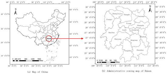
Figure 1.
Schematic diagram of study area.
Moreover, as can be seen from Figure 2, a collection of related datasets are collected from the traffic management bureau of the Hunan province: these include the expressway network, toll records, real-time surveillance data (license plate recognition devices, traffic flow observation stations, etc.), and GPS trajectory datasets. The period of all data covers the entire month of January 2018; during this period, severe traffic congestion occurred on the expressway due to extensive holiday-related travels (e.g., on New Year’s Day).
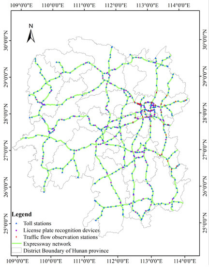
Figure 2.
The express highway network and different observation stations.
2.1. The Expressway Network
At the end of 2018, the total mileage of the expressway in the Hunan province of China had reached 6724.5 km. Since the expressway is a closed network, and all vehicles travelling through this network can only enter and exit through toll stations, the expressway network can be abstracted into a directed graph structure, i.e., the expressway network G = (V, E), with a set of nodes V and directed edges E.
There are 530 edges and 490 vertexes in the simplified expressway graph, as illustrated in Figure 2. Each edge e = (r, s)∈E has one properties cost d(r, s), which represents the length of the edge.
2.2. The Travel Toll Records
Time-varying traffic demand data has an important impact on the results of traffic assignment. Existing methods for traffic demand data collection can be classified into two types: survey-based [40] and traffic surveillance [41,42,43,44]. The former has been gradually replaced by the latter due to the former’s high labor costs, limited coverage, and strong subjective nature.
Here, the expressway toll records are collected to estimate the required time-varying traffic demand. Each record has six attributes: vehicle ID, entry and exit station codes, entry and exit time, and vehicle class. There are about 23 million toll records for January of 2018, three samples of which are listed in Table 1.

Table 1.
Sample toll records.
Since a given trip on one day may extend past the midnight, two different cases in the toll records need to be processed separately for traffic demand extraction. The first case is when the entry time and exit time are both within a single day, meaning that all records are extracted as valid OD pairs. The second case is when the entry and exit times are on different days separately; under these circumstances, records in which less than half of the total travel time elapses on this day will be discarded.
2.3. Real-Time Surveillance Data
Two types of real-time surveillance data are involved here: namely, license plate recognition (LPR) data and link flow observation data.
The LPR data is obtained by traffic surveillance cameras located at the chosen links of the expressway network (shown in Figure 2). An LPR record will be generated when the vehicle’s license plate is recognized by the installed camera. The record consists of the vehicle ID, site code, record time, and driving direction. There are about 72 million LPR records for January of 2018, three of which are presented in Table 2.
Table 2.
Sample data of LPR.
There are a total of 38 traffic flow observation stations installed in the chosen study area (shown in Figure 2). The link flow data obtained by traffic flow observation stations can be used to validate the accuracy of the proposed assignment models. All records of traffic flow with different vehicles classes are generalized into a single unit, named the passenger car unit (PCU); moreover, the real daily traffic volume of links is within the range of 1000 and 200,000.
2.4. The GPS Trajectory Dataset
Road traffic conditions reflect the congestion level of each road segment, which can in turn be used to calculate the time-dependent link cost (i.e., travel time) with reference to the relationship between road conditions and free flow speed. With the development of intelligent navigation maps, historical or real-time road condition data can now be easily obtained from the remote access interface of online map systems such as Google Maps, etc.
Here, the GPS trajectories collected from 37,221 special-purpose vehicles during January 2018 are used to calculate the time-dependent link cost (i.e., buses, trucks). There are approximately 1.84 billion records in total, and the data frequency is about one GPS point every 10~30 s. Each record contains six attributes: vehicle ID, timestamp, longitude, latitude, instantaneous velocity, and direction.
Before importing GPS trajectory data into our model, it is first necessary to process the GPS trajectory dataset. Initially, the duplicated GPS points in each GPS trajectory are removed; subsequently, the GPS points are matched to the road network using the ST-matching algorithm [45]. Finally, GPS trajectories comprising more than five points are reserved to avoid the interference caused by GPS points that are not located in the selected expressway.
3. Methods
Figure 3 outlines the framework of the proposed DQ-DTA model, which is extended from the general framework of a macroscopic DTA model. It appends two novel components: dynamic link cost calculation (DLC) and multipath assignment based on statistical probability (MSP).
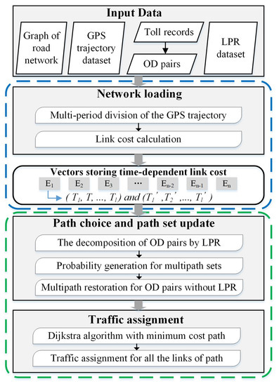
Figure 3.
The overall framework of the DQ-DTA model. The modules in the blue and green dashed boxes represent the dynamic link cost calculation (DLC) and multipath assignment based on statistical probability (MSP) methods respectively.
3.1. Dynamic Link Cost Calculation
BPR functions are typically used to estimate travel time from known traffic flow. However, the travel times do not follow a convex function with respect to flow [18], which leads to inaccurate travel time estimation, especially during traffic congestion. To overcome this shortcoming of BPR, GPS trajectory data can be employed to effectively reflect real-time traffic conditions; thus, they are used here to calculate the time-dependent travel time of the road network, i.e., DLC, which replaces the BPR function for the link cost calculation.
Following the fine-grained temporal segmentation in DTA, one day is divided into l time intervals. The GPS trajectory dataset then needs to be divided into l parts according to the time intervals. In each decomposed dataset of the GPS trajectory, the attribute of vehicle speed is used to calculate the average travel time for all links in a certain period. For example, if the link E (a, b) has k vehicles at a time period from a to b, the average travel speed and travel time of the current time period in this direction can be expressed by Equations (1) and (2) respectively:
where Vab is the average travel speed of link from node a to b; vji is the speed of vehicle j at GPS point i; mj is the total number of GPS points of vehicle j on link E(a, b); k is the total number of vehicles on link E(a, b); n is the total number of nodes in the expressway network; Tab is average travel time of link E(a, b); finally, Dab is the distance of E(a, b).
Hence, two average travel time vectors (i.e., upward and downward) of each link for each day can be obtained in l time intervals. For example, for the link E(a, b), the format of the time vector can be expressed in Table 3.
Table 3.
Travel time vector of one link E(a, b) by time interval.
3.2. Multipath Assignment Based on Statistical Probability
To overcome this shortcoming of logit-related models during multipath traffic assignment, LPR data can be used to constrain the path choice for OD pairs; this is done because the multipath sets of constrained OD pairs are much closer to the realistic path choices. Accordingly, utilizing massive amounts of travel history data provided by OD pairs and LPR records, a multipath assignment method based on statistical probability (MSP) can be defined to capture user route choices.
There are two types of OD pairs, namely those with and those without internal LPR records. The decomposition and probability generation procedure is applied for the former, while multipath restoration is used for the latter. Ultimately, all the results of prior processing are used for traffic assignment.
For OD pairs with internal LPR records, each pair is decomposed by LPR points according to the temporal order. In Figure 4, points S1 and S2 are the LPR points of one OD pair, where S1 belongs to link E(a, b) and S2 belongs to link E(p, q). The OD pair can thus be decomposed into five sub-OD pairs (o–a, a–b, b–p, p–q, and q–d), so that a detailed path of OD (o–a–b–p–q–d) can be derived.
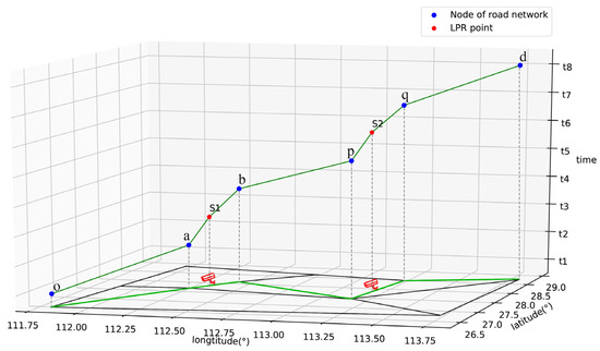
Figure 4.
An OD pair decomposed by LPR data.
Since the travel path choices differ depending on vehicle class, the OD pairs and the later path statistics are classified according to these vehicle classes. After decomposing these OD pairs containing the LPR points, the paths of the vehicles with the same class and the same OD are counted. For example, for the OD pair (r, s) with class i, one path hi, j of the multipath set hi and the probability (Pi, j) of path hi, j can be counted, which can be expressed in Equations (3)–(5) below. Moreover, the probability generation results of the OD pair (r, s) with class i are listed in Table 4.
Table 4.
One dataset of probability generation of the OD pair (r, s).
Here, N is the set of all nodes on the expressway network; C is a set of all classes of vehicles; m is the total path count for the OD pair (r, s) with vehicle class i; is the multipath set of the OD pair (r, s)with vehicle class i, while is the count of vehicle class i in path of the OD pair (r, s).
For OD pairs without internal LPR records, the results of probability generation (i.e., multipath sets and statistical probability) can be used to restore traveler route choices. These OD pairs are grouped into different sets depending on the vehicle class and counted with the same OD. The route choices of each OD set can then be restored by the multipath sets, such that the counts of each restored path are calculated by the product of the total count and the corresponding statistical probability. For example, vehicles of class A have 500 counts of OD pair (r, s); the results of multipath restoration are listed in Table 5.
Table 5.
Path restoration result of OD pair (r, s) by the probability.
During the traffic assignment, since the OD pairs are decomposed into a detailed path comprising certain sub-OD pairs, each sub-OD pair can be treated as an independent OD pair for processing. Initially, each sub-OD pair is divided into l discrete time intervals according to its entry and exit time. Next, the l weights of each time interval are calculated and set for the sub-OD pairs. Each weight wi is equal to the ratio of the travel time length in each discrete time interval to the total travel time. For example, consider a vehicle that enters the expressway at 13:30 on 1 January 2018 and exits the expressway at 15:30. If l is set to 24, the total duration of this sub-OD pair is 120 minutes; accordingly, the weight w13 = 0.25, w14 = 0.5, w15 = 0.25, while the other weights are 0.
To find the minimum cost path of each sub-OD pair,the link cost de of all links on the expressway needs to becalculated for the time period of the sub-OD pair. The time-dependent link cost
de can be updated using the weights w of each sub-OD pairand the variables of travel time vector Te to performweighted average summation. For example, for the sub-OD pair (r, a), thelink cost of all of its links can be calculated using Equation(6) below. The Dijkstra algorithm [6] is then usedto find the path with minimum cost, after which all links of the path areassigned the same traffic flow at the same time. Finally, the above steps arelooped for all sub-OD pairs.
Here, wi is the time weight ofthe sub-OD pair (r, a) in the time interval i; l is thetime interval size; is the travel time of the link e in thetime interval i; finally, is the dynamic link cost of edge ein the time intervals of the sub-OD pair (r, a).
In addition, since the structure of the expressway network is a directed graph, the assigned traffic volumes on the link also have directions (up and down) on the expressway network. Consequently, the total traffic volume of a link is the summation of all traffic volumes assigned in both directions of the link.
4. Results and Discussion
In order to evaluate the performance of our DQ-DTA model, we apply the proposed approach to the real large-scale expressway network in the Hunan province. Two experiments are conducted to compare the accuracy of different traffic assignment models, in which the proposed DQ-DTA model and four classical STA models (AON, Incremental, STOCH, and UE) are implemented.
4.1. Performance Comparison with Classical STA Models
Classical STA models provided by the TransCAD software package were used to assign the traffic flow, specifically AON, Incremental, STOCH, and UE. The assigned traffic flow of these STA models were then compared with the real traffic volumes recorded by traffic flow observation stations, after which the accuracy of the assignment is evaluated using the mean relative error (MRE), derived according to Equation (7):
where m is the number of real observation data, i.e., 38 here; moreover, yi is the assigned traffic flow of the link, while yir is the real traffic flow.
In this experiment, the time interval l of the DQ-DTA model is provisionally set to 24; the sensitivity of the value of l is analyzed in more detail below. The MRE values for these five models are plotted in Figure 5, from which it can be seen that the DQ-DTA model achieves the highest accuracy and an MRE of about 0.08. The performances of the four classical STA models are almost identical (i.e., around 0.15), while the MRE of the UE model, which performs better than the other classical models, is about 0.143. Thus, the accuracy of the proposed DQ-DTA model is about 6~7% higher than that of these STA models.
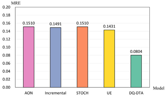
Figure 5.
The mean relative error of observed links of the four classical models and the DQ-DTA model on the expressway network.
In addition, the relative errors (RE) of all the chosen links among these five models are shown in Figure 6a,b, respectively. In Figure 6a, the relative errors of the four classical STA models generally fall between 0.04 and 0.2, while their maximum relative error is close to 0.78. However, the relative errors of the DQ-DTA model are mostly between 0.03 and 0.1, indicating that the MRE has been greatly improved. At the same time, the maximum relative error drops from 0.78 to 0.32. In the violin plots in Figure 6b, the relative errors of nearly all the links with the DQ-DTA model fall below 0.1, which indicating that the assignment quality have been greatly improved by the DQ-DTA model.
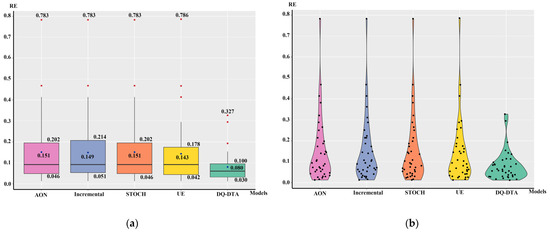
Figure 6.
(a) The box plot of relative error distribution of observed links for the four classical models and the DQ-DTA model; red and blue points mean outliers and mean, respectively. (b) The scatter and violin plots of the relative error distribution of observed links for the four classical models and the DQ-DTA model.
4.2. Ablation Study on the DQ-DTA
The UE model that achieves the best performance out of the classical STA models is chosen for comparison with the DLC, MSP, and DQ-DTA models in order to analyze the improvement achieved by these approaches. For the DLC, all initial OD pairs are used to assign directly the minimum link cost without decomposition of the OD pairs and multipath restoration. Likewise, for the MSP, the dynamic link cost calculation is replaced by calculating the shortest path according to the distance attribute of the expressway network.
The mean relative error and relative error distribution of the assigned results for the UE, DLC, MSP, and DQ-DTA models are plotted in Figure 7, Figure 8a, and Figure 8b. As the figures show, the DLC, MSP, and DQ-DTA models achieve a certain degree of improvement in terms of accuracy compared with the UE model; moreover, the DQ-DTA model, which combines both the DLC and MSP, scores the highest in terms of accuracy.
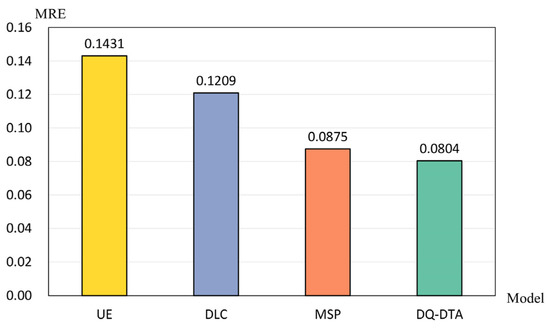
Figure 7.
The mean relative error of observed links by the UE, DLC, MSP, and DQ-DTA models.
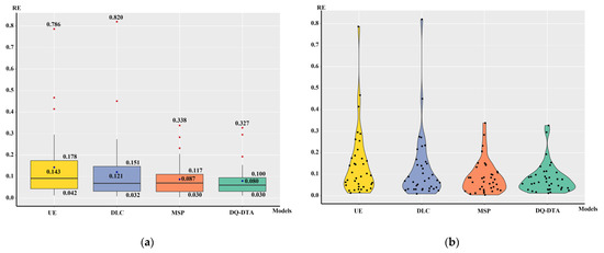
Figure 8.
(a) The box plot of relative error distribution of observed links of the UE, DLC, MSP, and DQ-DTA models; red and blue points mean outliers and mean, respectively. (b) The scatter and violin plots of the relative error distribution of observed links of the UE, DLC, MSP, and DQ-DTA models.
Moreover, the two links with the top two relative errors in the UE model (i.e., links 379 and 367) are chosen for further improvement analysis. The relative errors on the chosen two links for UE, DLC, MSP, and DQ-DTA are shown in Figure 9. First, MSP substantially reduces the relative error of link 379 from 0.467 to 0.338, while the DLC achieves only a slight improvement. Second, DLC greatly reduces the relative error of link 367 from 0.414 to 0.169; by contrast, MSP achieves only moderate improvement. Finally, the DQ-DTA model obtains the lowest relative error for links 379 and 367.
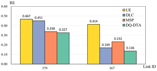
Figure 9.
The relative error on the chosen two links of the UE, DLC, MSP, and DQ-DTA models.
To explain the contribution difference of DLC and MSP between links 379 and 367, the road network connectivity and traffic congestion distribution of these two links are compared from a visual perspective in Figure 10. For link 379, the connectivity degrees of the two endpoints are higher in the road topology, and this means that there are more route choices through these intersections during the multi-path traffic assignment; thus, the MSP can improve the assigned result more significantly. At the same time, the traffic conditions of link 379 are less congested than that of link 367, as shown in Figure 10b, so the DLC achieves very little improvement. Likewise, for link 367, the DLC improves the assigned result more significantly due to the traffic condition being much poorer. In addition, although the connectivity degrees of link 367’s right endpoint are still high in the road topology, the route choices may be much reduced due to poor traffic conditions; consequently, while the MSP model achieves some improvement, it does not improve the assigned result as much as the DLC.
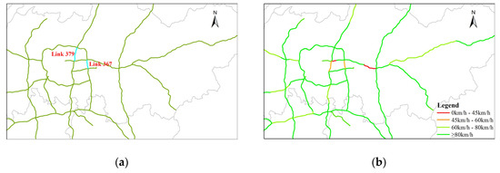
Figure 10.
Comparison of links 379 and 367 from a visual perspective. (a) Locations of links 379 and 367. (b) Traffic conditions near links 379 and 367 during the evening peak on 1 January 2018.
Overall, the ablation study of DLC, MSP, and DQ-DTA indicate that the DLC and MSP models improve the accuracy relative to the classical STA models to varying extents, while the DQ-DTA model can combine the superiority of both the DLC and MSP models to obtain the most accurate results.
4.3. Sensitivity Analysis
The sensitivity analysis determines how the MRE of assignment models changes with different time interval sizes in the DQ-DTA model. Six kinds of time granularity are chosen for the experiments: i.e., 1/4, 1/2, 1, 2, 3, and 6 hours. The sensitivity analysis results are listed in Figure 11.
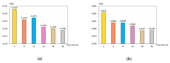
Figure 11.
Mean relative errors under the DLC and DQ-DTA models with different levels of time interval perturbation. (a) DLC model. (b) DQ-DTA model.
The mean relative errors of these two models are nearly proportional to the time interval size, which is in line with the actual situation of the dynamic time-varying nature of the DTA. As the time interval l increases, the MRE of the assigned results of DLC and DQ-DTA rapidly decrease when l is less than 24, then decrease more slowly when l exceeds 24. It can accordingly be concluded that the time interval size l can be set to 24 (i.e., one hour per time interval), which is appropriate for the actual large-scale expressway network. Furthermore, this value can strike a balance between computation time and accuracy.
5. Conclusions
In summary, a data-driven quasi-dynamic traffic assignment (DQ-DTA) model is proposed that integrates multi-source traffic sensor data for a large-scale expressway network. The expressway network, real-time toll records and LPR data, traffic flow observation stations, and GPS trajectory data are combined to accurately obtain the traffic demand, waypoints, real traffic volumes, and time-varying traffic condition. Furthermore, a dynamic link cost calculation method (DLC) based on GPS trajectory data is designed to replace the BPR function in order to calculate the link cost. Moreover, by combining the OD pairs and LPR data, a multipath assignment method based on statistical probability (MSP) is proposed to help in precisely restoring the user path choices. The results of the DQ-DTA model were verified using real link flow data from traffic flow observation stations; according to our experiments, the mean relative error is improved by nearly 6% compared to classical STA models. Furthermore, the model has low computing resource requirements, while its computational efficiency remains close to that of the STA models owing to the lack of iteration for calculation.
However, there are still some limitations of the DQ-DTA model that will be addressed in the near future.
- Our proposed approach only considers the time cost from traffic congestion during the link cost update. Other factors influencing travel costs, e.g., toll fees [7], weather conditions, and differences between week days/weekends should also be considered later.
- This model is currently applied only to the closed expressway networks. We will further apply our model into urban road networks, in which the openness of the road topology and signal light control [46,47] would increase the difficulty of both travel demand estimation and travel-time cost calculation. In addition, the complexity of road topological structure will also increase the computational complexity of traffic assignment models.
- With the development of the Internet of Things, other complex data-driven methods (e.g., deep learning) can be explored to address traffic assignment problems.
Author Contributions
Conceptualization: Xing Zeng and Xuefeng Guan; Methodology: Xing Zeng and Xuefeng Guan; Software: Xing Zeng; Validation: Xing Zeng and Xuefeng Guan; Formal Analysis: Xing Zeng; Investigation: Heping Xiao; Resources: Xuefeng Guan and Heping Xiao; Data Curation: Xing Zeng and Heping Xiao; Writing—Original Draft Preparation: Xing Zeng; Writing—Review & Editing: Xing Zeng, Xuefeng Guan, and Huayi Wu; Visualization: Xing Zeng; Supervision: Xuefeng Guan and Huayi Wu; Project Administration: Xuefeng Guan and Huayi Wu; Funding Acquisition: Xuefeng Guan and Huayi Wu All authors have read and agreed to the published version of the manuscript.
Funding
This research was funded by the National Key Research and Development Program of China, grant number 2017YFB0503802 and the National Natural Science Foundation of China, Grant number 41971348.
Informed Consent Statement
Informed consent was obtained from all subjects involved in the study.
Data Availability Statement
The data are not publicly available due to privacy.
Conflicts of Interest
The authors declare no conflict of interest.
References
- Nakayama, S.I.; Takayama, J.I.; Nakai, J.; Nagao, K. Semi-dynamic traffic assignment model with mode and route hoices under stochastic travel times. J. Adv. Transp. 2012, 46, 269–281. [Google Scholar] [CrossRef]
- Bliemer, M.C.; Raadsen, M.P.; Smits, E.-S.; Zhou, B.; Bell, M.G. Quasi-dynamic traffic assignment with residual point queues incorporating a first order node model. Transp. Res. Part B Methodol. 2014, 68, 363–384. [Google Scholar] [CrossRef]
- Tajtehranifard, H.; Bhaskar, A.; Nassir, N.; Haque, M.M.; Chung, E. A path marginal cost approximation algorithm for system optimal quasi-dynamic traffic assignment. Transp. Res. Part C Emerg. Technol. 2018, 88, 91–106. [Google Scholar] [CrossRef]
- Smith, M.; Huang, W.; Viti, F.; Tampère, C.M.; Lo, H.K. Quasi-dynamic traffic assignment with spatial queueing, control and blocking back. Transp. Res. Part B Methodol. 2019, 122, 140–166. [Google Scholar] [CrossRef]
- Jayakrishnan, R.; Tsai, W.K.; Chen, A. A dynamic traffic assignment model with traffic-flow relationships. Transp. Res. Part C Emerg. Technol. 1995, 3, 51–72. [Google Scholar] [CrossRef]
- Dijkstra, E.W. A note on two problems in connexion with graphs. Numer. Math. 1959, 1, 269–271. [Google Scholar] [CrossRef]
- Lee, E.; Oduor, P.G. Using multi-attribute decision factors for a modified all-or-nothing traffic assignment. Isprs Int. J. Geo-Inf. 2015, 4, 883–899. [Google Scholar] [CrossRef]
- Ferland, J.A.; Florian, M.; Achim, C. On incremental methods for traffic assignment. Transp. Res. 1975, 9, 237–239. [Google Scholar] [CrossRef]
- Flötteröd, G.; Rohde, J. Operational macroscopic modeling of complex urban road intersections. Transp. Res. Part B Methodol. 2011, 45, 903–922. [Google Scholar] [CrossRef]
- Irwin, N.; Dodd, N.; Von Cube, H. Capacity restraint in assignment programs. Highw. Res. Board Bull. 1961, 297, 109–127. [Google Scholar]
- Dial, R.B. A probabilistic multipath traffic assignment model which obviates path enumeration. Transp. Res. 1971, 5, 83–111. [Google Scholar] [CrossRef]
- Florian, M.; Fox, B. On the probabilistic origin of dial’s multipath traffic assignment model. Transp. Res. 1976, 10, 339–341. [Google Scholar] [CrossRef]
- Wardrop, J.G. Road paper. Some theoretical aspects of road traffic research. Proc. Inst. Civ. Eng. 1952, 1, 325–362. [Google Scholar] [CrossRef]
- Brederode, L.; Pel, A.; Wismans, L.; de Romph, E.; Hoogendoorn, S. Static traffic assignment with queuing: Model properties and applications. Transp. A: Transp. Sci. 2019, 15, 179–214. [Google Scholar] [CrossRef]
- Flügel, S.; Flötteröd, G. Traffic assignment for strategic urban transport model systems. In Proceedings of the ITEA Conference, Oslo, Norway, 15–19 June 2015. [Google Scholar]
- Marshall, N.L. Forecasting the impossible: The status quo of estimating traffic flows with static traffic assignment and the future of dynamic traffic assignment. Res. Transp. Bus. Manag. 2018, 29, 85–92. [Google Scholar] [CrossRef]
- Systematics, C. Travel Demand Forecasting: Parameters and Techniques; Transportation Research Board: Washington, DC, USA, 2012; Volume 716. [Google Scholar]
- Saw, K.; Katti, B.; Joshi, G. Literature review of traffic assignment: Static and dynamic. Int. J. Transp. Eng. 2015, 2, 339–347. [Google Scholar]
- Han, L.; Sun, H.; Wang, D.Z.; Zhu, C. A stochastic process traffic assignment model considering stochastic traffic demand. Transp. B Transp. Dyn. 2018, 6, 169–189. [Google Scholar] [CrossRef]
- Cascetta, E.; Nuzzolo, A.; Russo, F.; Vitetta, A. A modified logit route choice model overcoming path overlapping problems. Specification and some calibration results for interurban networks. In Proceedings of the 13th International Symposium on Transportation And Traffic Theory, Lyon, France, 24–26 July 1996. [Google Scholar]
- Cascetta, E.; Russo, F.; Viola, F.A.; Vitetta, A. A model of route perception in urban road networks. Transp. Res. Part B Methodol. 2002, 36, 577–592. [Google Scholar] [CrossRef]
- Bovy, P.H.; Bekhor, S.; Prato, C.G. The factor of revisited path size: Alternative derivation. Transp. Res. Rec. 2008, 2076, 132–140. [Google Scholar] [CrossRef]
- Vitetta, A. A quantum utility model for route choice in transport systems. Travel Behav. Soc. 2016, 3, 29–37. [Google Scholar] [CrossRef]
- Li, C.; Anavatti, S.G.; Ray, T. A path-based solution algorithm for dynamic traffic assignment. Netw. Spat. Econ. 2017, 17, 841–860. [Google Scholar] [CrossRef]
- Hu, T.Y.; Tong, C.C.; Liao, T.Y.; Chen, L.W. Dynamic route choice behaviour and simulation-based dynamic traffic assignment model for mixed traffic flows. Ksce J. Civ. Eng. 2018, 22, 813–822. [Google Scholar] [CrossRef]
- Zhang, L.; Liu, J.; Yu, B.; Chen, G. A dynamic traffic assignment method based on connected transportation system. IEEE Access 2019, 7, 65679–65692. [Google Scholar] [CrossRef]
- Javani, B.; Babazadeh, A.; Ceder, A. Path-based capacity-restrained dynamic traffic assignment algorithm. Transp. B Transp. Dyn. 2019, 7, 741–764. [Google Scholar] [CrossRef]
- Peeta, S.; Ziliaskopoulos, A.K. Foundations of dynamic traffic assignment: The past, the present and the future. Netw. Spat. Econ. 2001, 1, 233–265. [Google Scholar] [CrossRef]
- Szeto, W.; Lo, H.K. Dynamic traffic assignment: Properties and extensions. Transportmetrica 2006, 2, 31–52. [Google Scholar] [CrossRef]
- Chiu, Y.; Bottom, J.; Mahut, M.; Paz, A.; Balakrishna, R.; Waller, T.; Hicks, J. Transportation Research Circular e-c153: Dynamic Traffic Assignment: A Primer; Transportation Research Board of the National Academies: Washington, DC, USA, 2011. [Google Scholar]
- Huang, W.; Song, G.; Hong, H.; Xie, K. Deep architecture for traffic flow prediction: Deep belief networks with multitask learning. IEEE Trans. Intell. Transp. Syst. 2014, 15, 2191–2201. [Google Scholar] [CrossRef]
- Lv, Y.; Duan, Y.; Kang, W.; Li, Z.; Wang, F. Traffic flow prediction with big data: A deep learning approach. IEEE Trans. Intell. Transp. Syst. 2014, 16, 865–873. [Google Scholar] [CrossRef]
- Chao, K.H.; Chen, P.Y. An intelligent traffic flow control system based on radio frequency identification and wireless sensor networks. Int. J. Distrib. Sens. Netw. 2014, 10, 694545. [Google Scholar] [CrossRef]
- Xia, Y.; Shi, X.; Song, G.; Geng, Q.; Liu, Y. Towards improving quality of video-based vehicle counting method for traffic flow estimation. Signal Process. 2016, 120, 672–681. [Google Scholar] [CrossRef]
- Heilmann, B.; El Faouzi, N.E.; de Mouzon, O.; Hainitz, N.; Koller, H.; Bauer, D.; Antoniou, C. Predicting motorway traffic performance by data fusion of local sensor data and electronic toll collection data. Comput. Aided Civ. Infrastruct. Eng. 2011, 26, 451–463. [Google Scholar] [CrossRef]
- Wang, P.; Lai, J.; Huang, Z.; Tan, Q.; Lin, T. Estimating traffic flow in large road networks based on multi-source traffic data. IEEE Trans. Intell. Transp. Syst. 2020. [Google Scholar] [CrossRef]
- Anda, C.; Erath, A.; Fourie, P.J. Transport modelling in the age of big data. Int. J. Urban Sci. 2017, 21, 19–42. [Google Scholar] [CrossRef]
- Cascetta, E. Transportation Systems Analysis: Models and applications; Springer Science & Business Media: New York, NY, USA, 2009; Volume 29. [Google Scholar]
- Croce, A.I.; Musolino, G.; Rindone, C.; Vitetta, A. Sustainable mobility and energy resources: A quantitative assessment of transport services with electrical vehicles. Renew. Sustain. Energy Rev. 2019, 113, 109236. [Google Scholar] [CrossRef]
- Nie, Y.M.; Zhang, H.M. A variational inequality formulation for inferring dynamic origin–destination travel demands. Transp. Res. Part B Methodol. 2008, 42, 635–662. [Google Scholar] [CrossRef]
- Kim, J.; Kurauchi, F.; Uno, N.; Hagihara, T.; Daito, T. Using electronic toll collection data to understand traffic demand. J. Intell. Transp. Syst. 2014, 18, 190–203. [Google Scholar] [CrossRef]
- Lu, Z.; Meng, Q.; Gomes, G. Estimating link travel time functions for heterogeneous traffic flows on freeways. J. Adv. Transp. 2016, 50, 1683–1698. [Google Scholar] [CrossRef]
- Li, X.; Kurths, J.; Gao, C.; Zhang, J.; Wang, Z.; Zhang, Z. A hybrid algorithm for estimating origin-destination flows. IEEE Access 2017, 6, 677–687. [Google Scholar] [CrossRef]
- Nie, L.; Li, Y.; Kong, X. Spatio-temporal network traffic estimation and anomaly detection based on convolutional neural network in vehicular ad-hoc networks. IEEE Access 2018, 6, 40168–40176. [Google Scholar] [CrossRef]
- Lou, Y.; Zhang, C.; Zheng, Y.; Xie, X.; Wang, W.; Huang, Y. Map-matching for low-sampling-rate gps trajectories. In Proceedings of the 17th ACM SIGSPATIAL International Conference on Advances in Geographic Information Systems, Seattle, WA, USA, 4 November 2009; pp. 352–361. [Google Scholar]
- Webster, F.V. Traffic Signal Settings; Transportation Research Board: Washington, DC, USA, 1958. [Google Scholar]
- Akcelik, R. Traffic Signals: Capacity and Timing Analysis; Transportation Research Board: Washington, DC, USA, 1981. [Google Scholar]


Publisher’s Note: MDPI stays neutral with regard to jurisdictional claims in published maps and institutional affiliations. |
© 2021 by the authors. Licensee MDPI, Basel, Switzerland. This article is an open access article distributed under the terms and conditions of the Creative Commons Attribution (CC BY) license (http://creativecommons.org/licenses/by/4.0/).