Article

A Framework of Dam-Break Hazard Risk Mapping for a Data-Sparse Region in Indonesia

Center of Water Resources Engineering, Department of Civil Engineering, Parahyangan Catholic University, Jl. Ciumbuleuit 94, Bandung 40141, Indonesia
*
Author to whom correspondence should be addressed.
ISPRS Int. J. Geo-Inf. 2021, 10(3), 110; https://doi.org/10.3390/ijgi10030110
Submission received: 24 November 2020 / Revised: 26 January 2021 / Accepted: 8 February 2021 / Published: 26 February 2021

Abstract

:
This paper introduces a new simple approach for dam-break hazard mapping in a data-sparse region. A hypothetical breaching case of an earthen dam, i.e., the Ketro Dam in Central Java, (Indonesia) was considered. Open-access hydrological databases, i.e., TRMM and CHIRPS, were collected and compared with the rainfall ground station data to ensure data quality. Additionally, the 3-h rainfall distribution of the TRMM database was employed and validated with the measured data to establish the 24-h rainfall distribution of the probable maximum precipitation. The probable maximum flood discharge was computed with the SCS method, and the reservoir routing computation was conducted to determine the possible breaching mechanisms. The result shows that the Ketro Dam proves safe against overtopping, and thus only the piping mechanism has been taken into consideration. Using the breaching hydrograph, the open-access Digital Elevation Model MERIT Hydro, and the high-performance shallow water model NUFSAW2D, the flood propagation to the downstream part of the dam was simulated, enabling fast computations for different scenarios. The quantification of the susceptibility rate of urban areas was eased with overlay analysis utilizing InaSAFE, a plugin for the QGIS model. This study shows that even for a data-sparse region, the recent open-access databases in terms of hydrological and hydraulic aspects may be used to generate a dam-break hazard map. This will benefit the related stakeholders to take proper action to reduce the loss of life.

1. Introduction

Dam-break is one of several hazardous events that must be faced by Indonesia, especially when considering the existence of numbers of old dams. It is known that when a dam breaks, it instantaneously releases a large amount of water to its downstream areas, thus endangering not only human life, but also the economy and damaging property. Dam-break cases may be triggered by several factors, e.g., earthquakes and heavy rainfall, and therefore the design of dams is subjected to the recent construction code and standards that take such factors into account, despite a low probability of exceedance. In other words, assuming no construction mistake, dams are theoretically safe from a breach event, as long as the value of the design earthquake or flood is not exceeded. While new dams are subjected to the recent construction code, old dams may no longer meet the current safety standards due to their material quality degradation over time. Another complex factor such as climate change may have caused the parameter designs for such old dams to change dramatically. In addition, the control and regulation by the related stakeholders may not always function well, causing poor quality maintenance.
To the best of our knowledge, there has been two dam-break cases in Indonesia in the last decade. The first case occurred in 2009, where the Gintung Dam, built in 1933, broke and suddenly released approximately 2 million m3 of water to its downstream area [1]. It was reported that 100 people died, approximately 100 people went missing, and a total of 10 ha of the downstream area was inundated. This phenomenon has shown that the Gintung Dam, despite being a small dam with an approximate height of 6 m, was very dangerous as it broke. The second event occurred in 2013, where the Way Ela Dam—a dam naturally formed in 2012 due to the cliff landslide that blocked the main river—broke and suddenly released approximately 20 million m3 of water to its downstream area. According to the work in [2], the Way Ela Dam was approximately 35 m high and caused one person’s death, one person to go missing, and 32 people to become injured. Interestingly enough, the Gintung Dam, albeit smaller, was more hazardous than the Way Ela Dam. One of the reasons was the absence of the Emergency Action Plan (EAP) that had not been comprehensively considered yet in Indonesia before the Gintung dam-break event as a standard component in a dam-break risk assessment. Therefore, a comprehensive study of a dam-break risk evaluation is of paramount importance to reduce the risk to human life as well as the economy and damage to property.
In most developed countries, flood forecasts and early-warning systems have become a mandatory component in a flood EAP, which includes in particular flood hazard risk for spatial planning, property-level mitigation and preparedness measures, the maintenance of flood control systems, and effective disaster responses, see the works in [3,4,5,6]. In the scope of flood forecasts, most developed countries were supported by comprehensive databases including digital maps, hydrology data, river discharge measurements, and flood depth records, thus allowing one to calibrate as well as validate the results and making the flood hydrograph prediction more accurate. Currently, a comprehensive dataset of digital map is available for European countries, e.g., TanDEM-X (TerraSAR-X add-on for Digital Elevation Measurement) [7] that provides a database for a high-resolution Digital Elevation Model (DEM) up to 12 m horizontal accuracy and 2–4 m vertical accuracy, which was made possible by German Aerospace Center (DLR) and EADS Astrium (Airbus Defense and Space). Using a high-resolution DEM, one may perform a spatial hydrology analysis more properly. The high-resolution version of TanDEM-X is, however, not publicly available. In Bhola et al. [8], a comprehensive dataset of flood discharge measurement for White Main (Ködnitz) and Schorgast (Kauerndorf) Rivers was shown useful to develop a framework of offline flood inundation forecasts in Kulmbach City (Germany).
In many developing countries and data-sparse regions, such as Indonesia, a comprehensive flood database is often unavailable. Essentially, hydrograph data from a direct measurement are preferred for flood preventive measures. Using such direct hydrograph data helps one produce a more reliable result for flood simulations with a hydrodynamic model, rather than using the hydrograph computed from a Synthetic Unit Hydrograph (SUH) method, for instance. However, in every region in Indonesia, the direct hydrograph data are not completely available. Similar to rainfall data, there are only a few basins equipped with sufficient rainfall stations, while most are ungauged. In many cases, the rainfall data are very limited or missing. To deal with this issue, satellite-based data have recently been employed to estimate the hourly rainfall distribution.
The case study in this paper is the Ketro Dam, which is located in Central Java Province (Indonesia). It is an old dam and was built in 1984 [9]. The geographic position is at 7°02′11″ S and 110°55′42″ E, see Figure 1. The dam serves to supply water for the irrigation area of 852 ha. The Ketro River flows to the dam and finally to the Bengawan Solo River (main river), located approximately 6 km downstream of the dam. This study aims to provide a framework of dam-break hazard risk mapping for the Ketro Dam by taking into account the use of a rainfall–runoff model in combination with satellite-based rainfall data to conduct the flood computation, the use of a high-performance parallelized shallow water model associated with a reliable DEM to promote dam-break analysis, and finally the implementation of the QGIS model to allow for the quantification of hazard and susceptibility rate of urban areas at the downstream of the Ketro dam. It is expected that the method presented in this study would be beneficial and applicable in any other regions, especially in data-sparse areas.

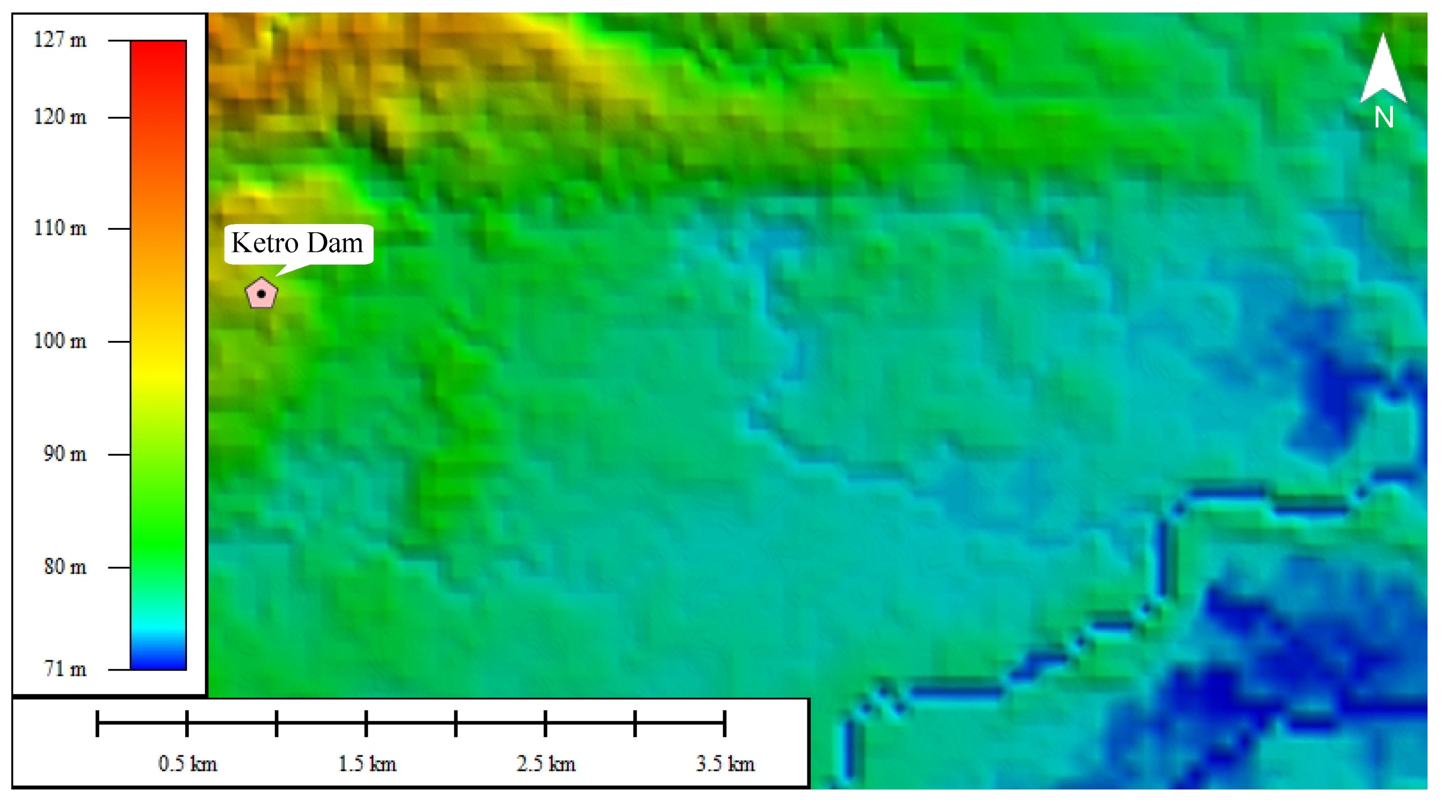
2. Description of Case Study: Ketro Dam

2.1. Technical Data of the Dam

The Ketro Dam is a homogeneous earthen dam with a total length of 1200 m and a height of 11 m (elevation of +102 m). To discharge flood flow, it is equipped with an ogee spillway, with a length of 11 m and a crest elevation of +99 m. The reservoir characteristics are given in Figure 2, showing that the Ketro Dam has a storage capacity of about 2.9 million m3 for the elevation of +99 m. Approximately 0.017% of the capacity (471 m3) is estimated to be the dead storage, which is located at an elevation of +91 m.

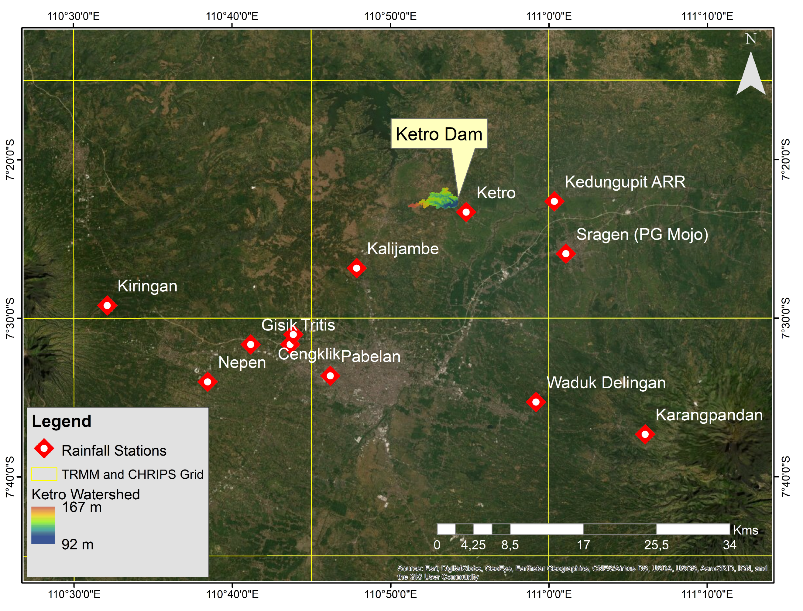
2.2. Catchment Area, Rainfall Data, and Other Measurement Values

The Ketro Dam has a catchment area of approximately 7.3 km2. As shown in Figure 3, it is obvious that the Ketro watershed is spatially represented by the rainfall data measured at the Ketro rainfall station. The available daily rainfall data (2009–2018) were collected from the official institution but without hourly rainfall distribution. In addition to the ground station data, the rainfall satellite data from TRMM (Tropical Rainfall Measuring Mission) and CHIRPS (Climate Hazards Group InfraRed Precipitation with Station data) databases were also collected. The TRMM and CHIRPS data were obtained for 2009–2018. Both of these data are of 0.25 degree resolution. Note that despite having a coarser resolution than the catchment area, see Figure 3, such data are still used to compare and check the quality of the ground station data.
The TRMM data are presented from the 3-h rainfall data, whereas the CHIRPS data are derived from the 24-h rainfall data. Note that as no hourly rainfall distribution is available for the ground station data, the distribution from the TRMM database will be used later for the flood hydrograph computations. To provide a representative view for the three groups of data, the maximum daily rainfall for each year is presented in Figure 4, showing that the rainfall ground station data tend to exhibit larger values than the others. It can also be seen that the discrepancy between the ground station and the TRMM values is larger, almost twice that between the ground station and the CHIRPS values. Despite the large discrepancy, all data are still employed and analyzed to discover the correlation between them. This will be explained in detail in Section 4.1. Finally, the measured discharge and water elevation at the dam for 2010–2018 are shown Figure 5, which will be used to calibrate and validate the SCS method for the flood hydrograph computations.

2.3. Land Use Map

In Figure 6, the land use map for the area downstream of the dam is given, showing that the land use pattern is also dominated by agriculture (cropland). Approximately 6 km downstream of the Ketro Dam, the main river (Bengawan Solo) flows from south to east. To determine the Manning coefficients that correspond to each land use type, a value range suggested in Bhola et al. [8] is employed and given in Table 1.

3. Methodology

3.1. Hydrology Data Uncertainty Analysis

The analysis framework in this study is initiated by assessing the rainfall data quality, as the considered precipitation data involves point (rainfall station) and grid data (TRMM and CHIRPS). Following McMillan et al. [10], the hydrology data involve several aspects of uncertainty, one of which is the data interpolation factor, where point and grid-based data matters. Moreover, there are other uncertainties factor considered, for example, data measurement, data transformation, and especially data scaling, as the size of the grid data and the catchment studied in this paper are found in a significantly different magnitude.
We appraise the quality control by quantifying each rainfall uncertainty estimation using the Extended Triple Collocation (ETC) method developed in McColl et al. [11]. Such a method is widely known to evaluate the data uncertainty by estimating the correlation coefficient with respect to the unknown true value and to quantify them using the objective functions Root Mean Square Error ( R M S E ) and r 2 [12]. In principle, the ETC method (as well as Classic Triple Collocation) assumes the existence of the linear relationship between the independent dataset X i and the hypothetical true value T as
X i = α i + β i T + ϵ i ,
where α i and β i are the calibration parameters, and ϵ i is the corresponding random error. Further, the covariances between different measurements are calculated by
P i , j = COV X i , X j = E X i , X j E X i E X j ,
where P i , j represents the covariance between two datasets X i and X j . Finally, the objective functions R M S E and r 2 can be calculated based on the covariances as follows:
R M S E 2 = P 1 , 1 P 1 , 2 P 1 , 3 P 2 , 3 P 2 , 2 P 1 , 2 P 2 , 3 P 1 , 3 P 3 , 3 P 1 , 3 P 2 , 3 P 1 , 2 , r 2 2 = P 1 , 2 P 1 , 3 P 1 , 1 P 2 , 3 P 1 , 2 P 2 , 3 P 2 , 2 P 1 , 3 P 1 , 3 P 2 , 3 P 3 , 3 P 1 , 2 ,
where each element in the matrix represents the objective function for each dataset.

3.2. Flood Discharge Design

The hydrology analysis starts from the determination of design rainfall for several return periods, including the probable maximum precipitation (PMP). This can be performed using a frequency analysis, e.g., log-normal, log-Pearson, or Gumbel distribution, which is then followed by the methods of goodness of fit test such as chi-square and Kolmogorov–Smirnov [13], using the following formula:
PMP = X ¯ n + R m · σ n ,
where X ¯ n and σ n are the mean and standard deviation of precipitation series for the n years of data, respectively. In this study, using the selected rainfall dataset, the PMP value is calculated using the Hershfield method [14,15], formulated as
R m = X m X ¯ n 1 σ n 1 ,
where R m is the statistical representation of the maximum value in the observed storm series, X m is the maximum observed storm value, X ¯ n 1 and σ n 1 are the mean value and standard deviation computed value excluding the largest one, respectively.
Typically, the rainfall data available in Indonesia provide only the maximum daily rainfall values without any information of the hourly rainfall distribution. Thus, the calculated PMP value is known to its daily total magnitude but remains undefined on its temporal distribution. Assuming a certain rainfall distribution, the computed design rainfall is commonly employed as an input for widely used SUH methods in Indonesia according to the current Indonesian standard [13], i.e., Snyder [16], Soil Conservation Service (SCS) [17,18,19], and Gama-I [20,21] methods, resulting in three hydrograph curves for each return period. According to the project reports [9,22,23], as in most cases no discharge measurement data are available for validation purposes, engineers frequently choose the hydrograph curve that gives the largest peak discharge. According to this study, this is, however, not a proper way of determining the curve that can closely represent the actual field condition. First, a detailed investigation should be conducted to obtain an appropriate hourly rainfall distribution. Second, the flood hydrograph curves resulted from the SUH methods should be assessed in detail with respect to the fairness and validity of the results. In this work, to check the quality of the ground station rainfall data as well as to appropriately decide the representative hourly rainfall distribution for the case study, the TRMM data [24] are utilized. The 3-h rainfall distribution of the TRMM database is used to construct the most appropriate distribution that can properly represent some past events with heavy rainfall data recorded.
Using the calculated PMP value and the calibrated rainfall distribution, the flood discharge is computed in this research based on the SCS method, to which the calibration of parameters and the validation of results are applied using the past flood events recorded at the dam location. This generally requires two data types: rainfall and curve number ( C N ) values. C N is an empirical parameter with respect to the hydrologic soil group and is used to estimate the direct runoff and the infiltration from the rainfall excess. The SCS method computes the peak runoff as
I p e a k = PMP A i n i t 2 PMP A i n i t + R p o t ,
where A i n i t is the initial abstraction and R p o t is the potential maximum retention after the runoff begins. The variables A i n i t and R p o t can be computed as
A i n i t = 0.2 R p o t , R p o t = 1000 C N 10 .
Equation (7) indicates that the unknown value of C N must be determined first to calculate the peak runoff in Equation (6). The lists of C N values are available in the literature [17,18,19], and for the sake of brevity are not shown here. In this study, the C N value is calibrated using the past rainfall event shown in Figure 5.

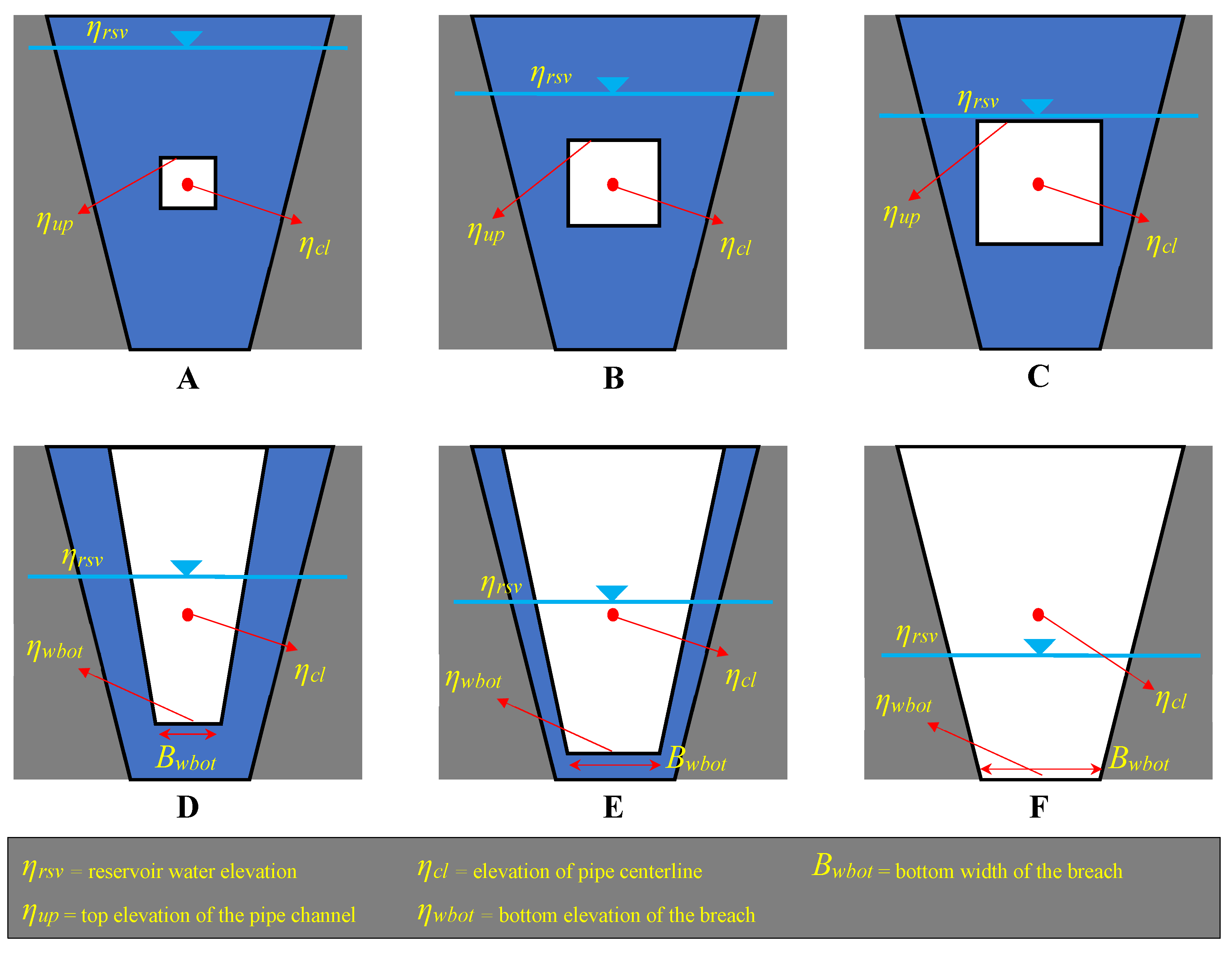
3.3. Breach Flow Computation

Another important aspect to be assessed in this work is the breach flow hydrograph, used as the main input to establish the inundation map for the downstream area of the dam. In this regard, two scenarios may be applied: dam-breach cases due to overtopping and piping. For the latter, further scenarios may be considered such as piping at the top, middle, and bottom locations of the dam. Extensive research has been conducted in the past to study the breach characteristics of earthen and rock-filled dams empirically including overtopping, piping, sliding, and wave action [25,26,27,28,29,30,31,32,33]. These studies resulted in several different empirical formulas for defining the peak breach discharge, the total breach time, and the final shape of the breach. However, the breach propagation from the initial phase to the final one is not available. Research has also been undertaken to study the physical processes of earthen dam-breach. These studies include physically based models and can be classified into two categories: numerical and simplified numerical models. The first category deals with fully hydrodynamic and sediment transport equations either a one-dimensional (1D), two-dimensional (2D), or three-dimensional (3D) model, see the works in [34,35,36]. The second category also considers the hydrodynamic and morphodynamic processes but with several simplifications and assumptions [37,38,39]. Note that the aforementioned 1D/2D/3D numerical models are so far only applicable to overtopping cases. In the case of a piping breach that includes both pipe and open-channel flow, the use of numerical models is still challenging, and thus the simplified numerical model may be used [40].
It is understood that despite playing an important role in characterizing the dam-breach properties, the empirical breach models may have several shortcomings, e.g., their high uncertainties and the neglect of the actual physical breach processes, and therefore one should consider using physically based models to account for the effect of soil properties on the breach propagation. However, the soil data are not comprehensively available for every project. This also means that the physically based models are not always applicable. In this work, as the soil data on the dam investigated were unavailable, the use of an empirical model becomes inevitable to predict the breach characteristics. The piping breach is assumed to linearly propagate from a rectangular hole to the final breach shape given in Froehlich [30]. The breach outflow is computed with both pipe and open-channel flow formulas.
The breach flow value depends on the initial water level and the reservoir volume when the dam breaks. In order to compute the change in the reservoir during breaching, the water level can be computed using the water balance equation as
d V r s v d t = I i n O b r c O s p i l l O s l u ,
where V r s v is the volume of reservoir, t is time, I i n is the inflow discharge, O b r c is the breach flow, O s p i l l is the spillway flow, and O s l u is the sluice flow. As no sluice gate is available at the Ketro dam, O s l u = 0 . The Froehlich formula [30] used in this work computes the breach characteristics including the total breach time and the shape of the breach as
B a v g = 0.27 k o V w t r 0.32 H b r c 0.04 , t b r c = 63.2 V w t r g H b r c ,
where B a v g is the average breach width, k o is a coefficient (1.3 for the overtopping case and 1 for the piping case), V w t r is the reservoir volume when breaching, H b r c is the breach height, and t b r c is the total breach time. The final shape of the breach is assumed to be trapezoid with the side slope z ( V : H = 1 : z ) being 1 for the overtopping case and 0.7 for the piping case.
Equation (9) is only applicable to determining the final shape of the breach, while the breach propagation was not clearly stated in Froehlich [30]. To the best of our knowledge, no empirical breach formulas have so far accounted for the breach propagation in detail. Therefore, a certain assumption for such propagation is required in order to define the breach flow hydrograph that will later be used for the flood inundation modeling. For this, a linear propagation mechanism as made in HECRAS Manual 5.0 [41] is employed here. Only the piping mechanism is given here because the Ketro Dam is safe against overtopping. This is shown in Figure 7. Note that O b r c for orifice flow (stages A–C) and for weir flow (stages D–F) are computed, respectively, as
O b r c = A b r c 2 g η r s v η c l 1 + f L o r f / B o r f ,
O b r c = 1 2 C d B w b o t + η r s v η w b o t tan α w b o t η r s v η w b o t 1.5 ,
where A b r c is the pipe cross-sectional area, η r s v is the reservoir water elevation, η c l is the elevation of the pipe centerline, f is the Darcy coefficient, L o r f is the length of the pipe channel, B o r f is the width of the pipe channel, C d is the weir discharge coefficient, B w b o t is the bottom width of the breach, η w b o t is the bottom elevation of the breach, and α w b o t is the side slope of the breach.
The processes in Figure 7 are explained as follows. Let us assume that the final breach bottom width is computed using Equation (9) to be B b o t . Assuming t b r c to be distributed into six stages, thus d t = t b r c / 6 , the breach bottom width at each stage equals ( d t B b o t / t b r c ). At the initial stage A, the hole is assumed to be a square with a width of ( d t B b o t / t b r c ) and a center coordinate specified as the initial piping elevation. The breach flow is computed using Equation (10) for the orifice flow mechanism. The reservoir water elevation is computed by solving Equation (8). At stage B, the hole grows larger linearly, thus the bottom width becomes ( 2 d t B b o t / t b r c ), again assuming that the reservoir water level, after solving Equation (8), is still higher than the top elevation of the hole. Similarly, stage C shows a linear growth of the hole with a bottom width of ( 3 d t B b o t / t b r c ), where the reservoir water level now equals the the top elevation of the hole. Note that stage C is the limit for the orifice flow type. Afterwards, the flow mechanism turns to the weir flow at stage D, where the breach shape now becomes trapezoid with a bottom width of B w b o t = 4 d t B b o t / t b r c . From this stage onward, the growth of the side slope of the trapezoidal breach is assumed to be linear. Now, the reservoir water elevation is computed by solving Equation (8) but the breach flow is calculated using Equation (11) for the weir flow mechanism. This process continues to occur to stage E, and finally, the final breach shape is obtained at stage F, where B w b o t = B b o t . Note that the change of mechanism from orifice to weir flow is governed by a criterion as [37]
η r s v < η c l + 2 η u p η c l ,
where η u p is the top elevation of the pipe channel.
The breach scenario is explained as follows. The dam-breach is considered to occur in two conditions: with and without rainfall. The former is expected to exist during the extreme rainfall (PMP), while the latter is to occur on a sunny day. The initial breach elevation for the former condition is assumed to begin at three elevation values: +100.5 m, +97 m, and +92 m that correspond to the elevation of the highest reservoir water level, the middle part of the dam, and the bottom part of the dam, respectively. For the latter condition, the initial piping elevation is at +99 m, which represents the elevation of the spillway crest. Note that each case for the former condition is assumed to exist when the reservoir water surface reaches the elevation of +100.5 m (the highest water elevation after the reservoir routing computation).

3.4. Mathematical Model of NUFSAW2D

Prior to quantifying the flood risk and impacts, a hydrodynamic model is required to estimate the inundated area downstream of the dam. For this, NUFSAW2D (Numerical simUlation of Free surface ShAllow Water 2D) developed by the second author of this paper is used. NUFSAW2D is an in-house code written for a set of solutions of the shallow water equations (SWEs) that has been extensively tested for numbers of hydraulic applications and was proven robust, accurate, and efficient. It has been applied to urban flood, dam-break, tsunami, turbulence modeling, and non-hydrostatic water–wave simulations, and works for structured and unstructured meshes [42,43,44,45,46,47,48,49,50,51]. Currently, NUFSAW2D is supported by a hybrid OpenMP-MPI parallelization.
For the sake of simplicity, only the basic formula (hydrostatic) of NUFSAW2D is employed and briefly described in this study, without the turbulence and non-hydrostatic terms. Thus, closely following Ginting [44], the SWEs are written as
Q t + C x x + C y y = S b x + S b y + S f ,
where Q denotes the conservative variables that depend on time t, C x and C y are the convective fluxes (or the convective terms), S b x and S b y denote the bed-slope terms, and S f defines the bed friction term. All the matrices are defined by
Q = h h u h v , C x = h u h u u + g h 2 2 h v u , C y = h v h u v h v v + g h 2 2 , S b x = 0 g h z b x 0 , S b y = 0 0 g h z b y , S f = 0 c f u ( u 2 + v 2 c f v ( u 2 + v 2 ,
where the variables h, u, and v are the depth and velocities in x and y directions, respectively; g is the gravity acceleration; z b is the bed contour; and n m is the Manning coefficient, where c f = g n m 2 h 1 3 . As a cell-centered finite volume (CCFV) Godunov scheme is used in this study, Equation (13) can be integrated over a sub-domain (a cell) Ω e by applying the Gauss divergence theorem, thus
A Ω e Q Ω e t + i = 1 N C x S b x n x + C y S b y n y i Δ L i = A Ω e S f Ω e ,
where n = n x , n y T is the unit normal vector pointing outward of the boundary and N is the total number of edges surrounding a cell. In this work, only simple rectangular cells are used to discretize a computational domain, thus N = 4 . The variable A Ω e is the area of sub-domain Ω e , and Δ L is the edge length.
It is known that the nonlinearity appears for the convective fluxes computations in Equation (15). For this purpose, a non-Riemann solver—central-upwind (CU) scheme originally developed by Kurganov et al. [52]—is used. To attain a second-order spatial accuracy, the Monotonic Upwind Scheme for Conservation Laws (MUSCL) method is employed for the reconstruction of the left (L) and right (R) states of an edge, prior to applying the CU scheme. The non-Riemann technique is also applied to the discretization of the bed-slope terms, while the bed friction term is computed using a semi-implicit treatment.
For the temporal discretization, the Runge–Kutta second-order (RKSO) method is employed and expressed as
K Ω e t = Δ t A Ω e i = 1 N C x S b x n x + C y S b y n y i t Δ L i , Q Ω e t = Q Ω e t + K Ω e t , Q Ω e t Π Ω e 1 Q Ω e t , Q Ω e t + 1 = 1 2 Q Ω e t + Q Ω e t + K Ω e t ,
where t and t denote the discrete time steps and Δ t is the time step size. The variable Π relates to the friction term S f Ω e and is calculated in a semi-implicit manner as
Π Ω e = 1 + g Δ t ( 1 θ ) n m 2 ( u 2 + v 2 h ( 4 3 Ω e t + θ n m 2 ( u 2 + v 2 h ( 4 3 Ω e ( t 1 ) ,
where θ is an implicitness coefficient (0 < θ < 1). The procedure of the semi-implicit treatment is briefly explained as follows. First, the computation is started by an explicit calculation of h Ω e t , h u Ω e t , and h v Ω e t in vector Q Ω e t ; note that no bed friction term is yet accounted for at this step. Second, dividing h u Ω e t and h v Ω e t with h Ω e t , both u Ω e t and v Ω e t are calculated; again, at this step, no bed friction term is considered yet. Finally, the bed friction term is computed to update the values of h u Ω e t and h v Ω e t as a final solution. For the sake of brevity, the computational details for both spatial and temporal discretization are not given here but are available in detail in the aforementioned NUFSAW2D’s publications [42,43,44,45,46,47,48,49,50,51].

3.5. Flood Risk Mapping

The final step is to quantify the flood risk and impacts on the potential losses of people, property, systems, or other elements subjected to the hazard zones. Currently, some methods are available to evaluate the risk of hazard events, in particular dam-break. A conceptual model to predict loss of life due to a dam-break case was developed in Brown et al. [53] based on the size of the population at risk and the amount of warning time possible for that population. In the scope of warning time and population at risk, Dekay et al. [54] extended the model in Brown et al. [53] to estimate the loss of life. Both of these models were based on empirical data, thus they may be inaccurate for other applications. Some models that combine multiple physical parameters have been developed in order to evaluate the risk of dam-break events [55,56,57]. Faster evaluation models [58,59] are also available, allowing engineers to identify, judge, and calculate the potential impacts of a single or multiple dam-break events. Even if the models [55,56,57,58,59] are readily applicable to general dam-break events, such models must be supported by advanced and comprehensive databases. In data-sparse regions, it is quite difficult to provide such databases.
In this study, a new simple approach for dam-break hazard mapping is developed, for which the recent open-access databases in terms of hydrological and hydraulic aspects may be used. To this regard, InaSAFE (Indonesian Scenario Assessment for Emergencies), an open-source plugin for QGIS (Quantum Geographic Information System) software, was employed to assess the susceptibility rate of the urban areas affected by the dam-break flood. InaSAFE was developed through a cooperation between the Indonesian government (Indonesian National Board for Disaster Management), the Australian Government, the World Bank-GFDRR (Global Facility for Disaster Reduction and Recovery), and independent contributors [60]. The results of InaSAFE are processed into a map that contains all spatial information related to the hazard, exposure, and aggregation components.
The flood management priority should be well defined so that the related stakeholders may take the proper actions, especially during the people evacuation. In this study, we develop a simple and effective method for the flood risk index by considering two main categories: (1) the dam-break flow characteristics and (2) the evacuation efficiency, combining the ideas of Wallingford [61] and Viseu et al. [62]. For each factor, there are several aspects considered, see Table 2. The first category takes three aspects into account: inundation depth, flow velocity, and debris carried by the flow. Meanwhile, the second category considers the evacuation efficiency related to the vulnerability index.
While the evacuation process will be conducted mostly by walking, the three aspects in the first category are considered because some people might be unaware that the velocity could be so strong as to sweep them, although the water depth is relatively low. Furthermore, the debris effect is taken into account as it may delay the walking process. From the first category, an index can be computed following Wallingford [61] as
F F = h × ( u 2 + v 2 + 0.5 + D F ,
where F F is the flood factor; h, u, and v are the depth and velocities computed using NUFSAW2D; and D F is the debris factor defined in Table 3. Note that 0.5 in Equation (18) is a velocity coefficient based on the experimental study [61].
In the original work of Wallingford [61], the degree of flood hazard was categorized into four classes (low, moderate, significant, and extreme), accounting for the components h × ( u 2 + v 2 + 0.5 only. In this study, we slightly modify the category by taking the component D F into account. For the sake of simplicity, 0.5 of D F is incorporated into the first two classes (low and moderate), whereas the rest is pointed to the others. One can define the flood hazard index ( F H I ) as given in Table 4.
For the second category in Table 2, three aspects are considered to assess the evacuation process efficiency: average distance to the evacuation place, vulnerable persons, and road to access the location of the evacuation place. The first aspect is obtained from the result of flood arrival time and evacuation place distance analysis; the second aspect from the total number of children, elderly, and disabled people aggregated from the field data; and the third one is from the site map. The next step is to define the proportion of each aspect for the value of the vulnerability index ( V I ). To the best of our knowledge, there have so far been no absolute criteria for determining V I as it may be solicited from expert judgments. For the sake of simplicity, the value of V I in this work is therefore devised as
V I = a 1 × D L + b 1 × V P + c 1 × L R ,
where a 1 , b 1 , and c 1 are coefficients; D L is a coefficient for average distance to the evacuation place; V P is a coefficient for the number of vulnerable persons; and L R is a coefficient for the length of the roads inundated. It follows that a 1 + b 1 + c 1 = 1 . Note that all the coefficients must be adjusted, thus posing a challenge. To keep the adjustment simple, we will correlate the coefficients a 1 , b 1 , c 1 , D L , V P , and L R with the values recorded for the case study. In other words, the values of the coefficients are subjected only to the Ketro Dam. The final index value is the flood risk level ( F R L ), computed from the values of F H I and V I , see Table 5.

4. Results and Analysis

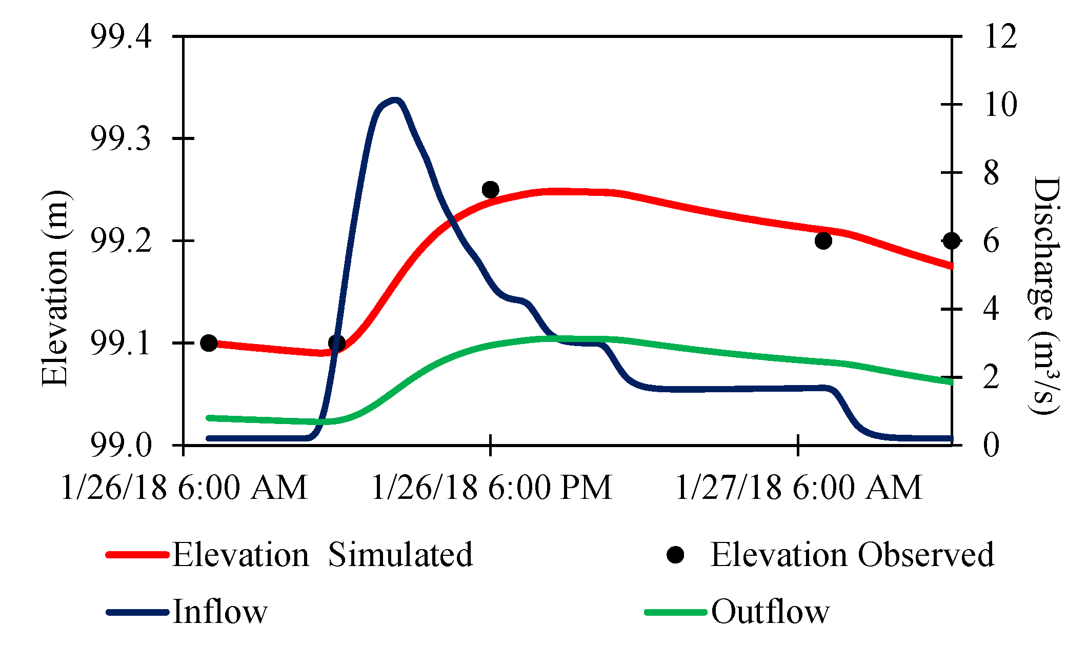
4.1. Hydrology Analysis

Applying the ETC method to all data (rainfall station, TRMM, and CHIRPS) delivers the results shown in Figure 8, indicating a better correlation between the TRMM and CHIRPS data than the rainfall ground station data. However, all results are produced in the low values of objective function. All r 2 values are less than 0.55, while the minimum R M S E value is 6.24 mm. This shows the existence of considerable uncertainties for all the point rainfall data, TRMM, and CHIRPS databases. Therefore, a qualitative analysis is required to choose the most appropriate data.
According to the uncertainties investigated in McMillan et al. [10], there exist, to a certain extent, uncertainties in the measurement for the rainfall station data and in the spatial scaling within the assumption of the data representativeness on the average rainfall values in the catchment. On the other side, the TRMM and CHIRPS data have more uncertainties (for data transformation and interpolation), in addition to the uncertainties in data measurement and data scaling, due to the data transformation from the raw measured variables. Following McColl et al. [11], if the ETC method gives R M S E 0 and/or r 2 1 for a rainfall database, the data should be chosen for the subsequent analysis. However, as shown in Figure 8, none of the databases provide the sufficient values of R M S E and/or r 2 . Therefore, the rainfall ground station data are used in this study because of the absence of data transformation and fewer data scaling uncertainties.
Using the data in Figure 4 and Equation (4) gives the PMP value of 503 mm. Further, the CN value must be calibrated for the SCS method, which is briefly explained as follows. From the TRMM database, the 108 mm rainfall event that occurred on 26–27 January 2018 and caused an increase of reservoir water level of 25 cm above the spillway crest is chosen. Using the TRMM’s 3-h rainfall distribution obtained on the date of the aforementioned event, an iterative procedure for the C N value is applied to the reservoir routing method (with the reservoir characteristic data in Figure 2) so that the computed reservoir water elevations can fit closely the measured ones. The calibration result is shown in Figure 9, which produces the C N value of 69.3 and indicates that the computed elevations are in agreement with the recorded ones.
In addition to the calibration process, a validation procedure is also carried out in this study to check whether the calibrated C N value is already an appropriate value. In this regard, another event from the TRMM database recorded on 15–16 December 2018 is chosen. This event was of 74 mm rainfall that caused an increase of the reservoir water level of 60 cm. Similar to the calibration process, using the TRMM’s 3-h rainfall distribution obtained on the date of this event, the SCS method is employed with the 74 mm rainfall to establish the flood hydrograph. Afterward, such a hydrograph is applied as an input to the reservoir routing method (with the reservoir characteristic data shown in Figure 2). The validation result is shown in Figure 10, which indicates that the computed reservoir water elevations conform with the measured ones. From all of these findings, it is therefore reasonable to say that 69.3 is the proper C N value.
Yet, the rainfall distribution for the PMP value, which is required to estimate the probable maximum flood (PMF) hydrograph using the SCS method, still remains unknown. Based on the standard code [13], one should consider for a PMP the longest rainfall event that ever occurred in the past events. To this regard, we again used the TRMM database to search the longest rainfall events that have ever existed near the Ketro Dam. The four longest rainfall cases were thus found, i.e., on 27 November 2017, 27 September 2016, 25 December 2007, and 20 June 2005 with the rainfall duration of 27 h, 24 h, 24 h, and 18 h, respectively. For this, several distribution types, i.e., 24-h Huff-1 [63], 24-h PSA07 [64], SCS I, SCS IA, SCS II, and SCS III [17], are tested and compared with the four data recorded. The results are shown in Figure 11, indicating that the 24-h Huff-1 distribution tends to be more suitable than the others for representing the recorded rainfall distribution due to the lowest average error of 8%. Therefore, the PMP value of 503 mm is, from now on, assumed to be distributed following the 24-h Huff-1 distribution.
The peak of the PMF hydrograph is computed to be 115 m3/s, and finally the final PMF hydrograph can be obtained with the 24-h Huff-1 distribution. Figure 12 shows the PMF hydrograph and its outflow after the reservoir routing calculation. One can see that the reservoir water reaches the maximum elevation of +100.5 m for the PMF event, denoting that the Ketro dam will be safe against the overtopping failure because the dam crest elevation is +102 m. Only the piping breaching scenario is thus considered for the subsequent analysis. Note that in order to account for the maximum inundation of the dam-breach event, the elevation of +100.5 m is chosen as the initial reservoir water level for all simulations.
The results of the computation for the final breach shape are summarized in Figure 13. Figure 14 shows the total flow hydrographs for all cases, which are the sum of breach flow and spillway flow. The peak discharges for the cases with the initial breach elevations of +100.5 m, +97 m, +92 m, and +99 m are 958 m3/s, 815 m3/s, 773 m3/s, and 652 m3/s, respectively.

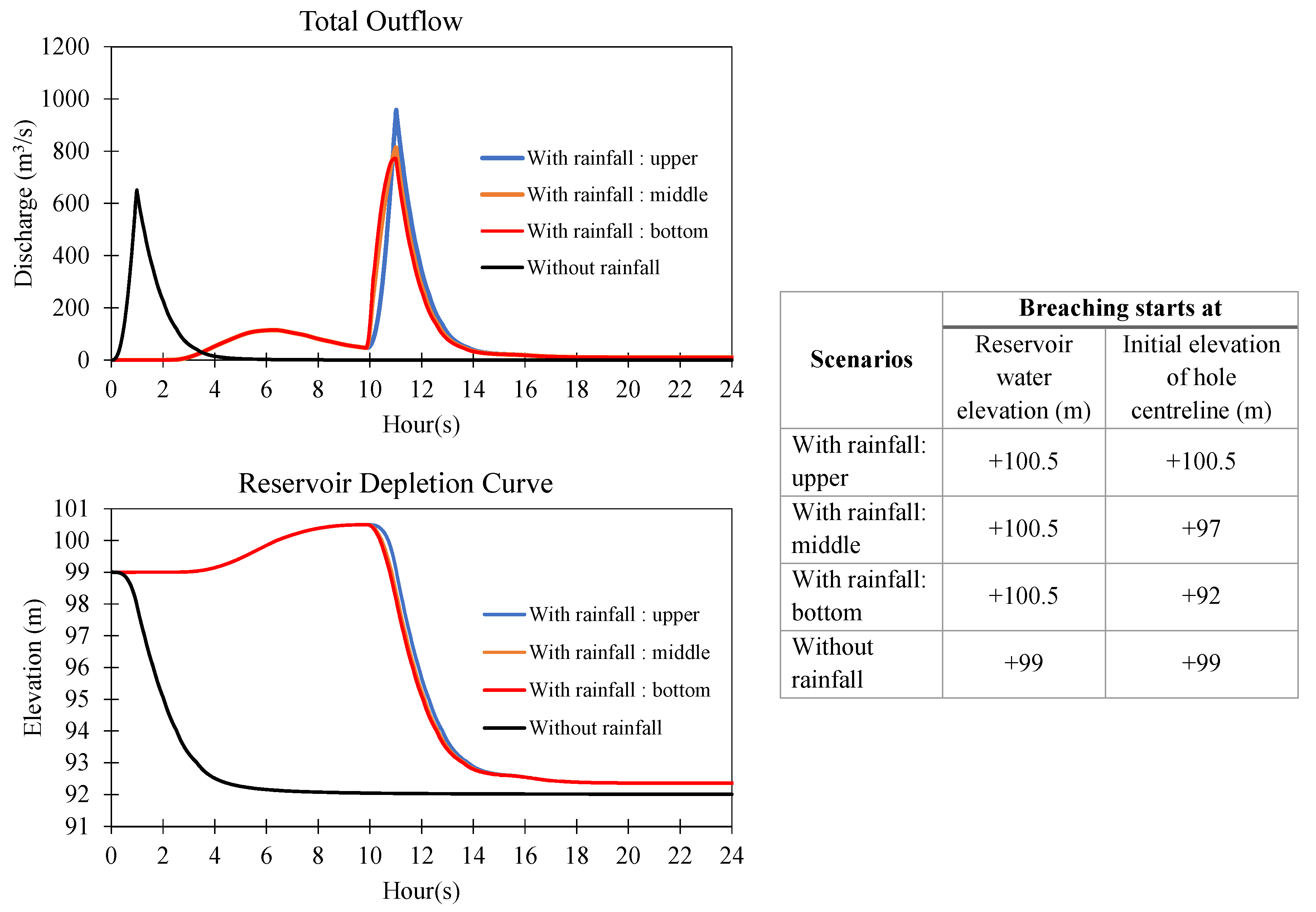
4.2. Flood Propagation Modeling

As no measured topography data are available for the area downstream of the dam, the flood simulation is carried out using an open-access DEM: MERIT (Multi-Error-Removed Improved-Terrain) Hydro, which was developed by Yamazaki et al. [65] and is freely available on the website [66]. MERIT Hydro has an accuracy of 3 arc-second resolution (90 m at the equator) and was developed specifically for hydrology and hydraulic analysis derived from the combination of the latest elevation data, i.e., MERIT DEM and water body datasets, e.g., G1WBM, GSWO (Global Surface Water Occurrence), and OpenStreetMap. It was noted in Saksena and Merwade [67] that two DEM attributes are important in flood modeling: horizontal and vertical accuracy. According to Hawker et al. [68], using low-resolution DEM (>30 m) may hamper an accurate estimation of flood hazard. In Azizian and Brocca [69], several DEMs from low- to high-resolution accuracy—e.g., SRTM (Shuttle Radar Topographic Mission) with 90 m and 30 m accuracy, ASTER (Advanced Spaceborne Thermal Emission and Reflection Radiometer) with 30 m accuracy, and ALOS (Advanced Land Observing Satellite) with 30 m accuracy—were used and compared for 1D flood simulations on rivers. It was found that the simulation with ALOS gave the best results among the others.
In our numerical experiments for this study, the use of ALOS and ASTER, however, led to an erroneous interpretation, where the flood water was detained near the downstream area of the dam and thus could not move elsewhere, even after 40 h of simulation time. This may be due to their characteristic of a Digital Surface Model (DSM) type that describes the top elevation of canopy and water surface, thus being unsuitable for flood simulations that require a type of Digital Terrain Model (DTM). While this issue may be problem-specific, and we therefore do not intend to discuss it here, MERIT Hydro, despite its low resolution, is used for all numerical simulations in this study. The main reason is that MERIT Hydro has been corrected and adjusted according to the hydrology and hydraulic features [65]. The visualization of the MERIT Hydro map is presented in Figure 15.
Several steps of the numerical simulations are explained as follows. First, the simulations are carried out using a constant outflow discharge, that is, the peak value obtained after the reservoir routing process for the inflow discharge with the high-probability event (1.5 years). This aims to obtain a steady flow condition as the initial condition for the dam-break simulations. Afterwards, the total outflow hydrograph shown in Figure 14 is used as the boundary flow condition. All simulations are carried out for the total simulation time of 40 h, thus representing the wetting and drying mechanisms. Note that only the results of the upper piping (with rainfall) case are shown in this paper because this mechanism gives the largest inundation area. The result of the numerical simulation using NUFSAW2D is shown in Figure 16.

4.3. Flood Risk Mapping Analysis

NUFSAW2D computes the flood characteristics including depth and velocity at every point of the discretized domain, where the results can easily be synergized into the framework of QGIS software utilizing the open-source plugin InaSAFE. This helps ease the spatial quantification of the flood effects, e.g., the number of population at risk, the potential property loss, etc. Three main data types—hazard (i.e., flood depth and velocity), exposure (i.e., the number of people and land use type), and aggregation (i.e., the administration border of areas)—must be provided prior to operating InaSAFE. In this regard, the flood depth values obtained from the numerical model are presented with respect to the maximum inundation area for 40 h of simulation time. The values of the flood depth are then categorized into three groups: <0.5 m, 0.5–1.5 m, and >1.5 m, see Figure 16.
In order to quantify the flood effects, we use the database from an open-source platform mapping OpenStreetMap (OSM) [70]. This platform collects the vital infrastructure data on a participatory basis from various sources including houses, roads, hospitals, schools, and others. The population data are obtained from an open source data [71], which has a spatial resolution of approximately 100 m × 100 m. In the first step, we intend to quantify the number of people at risk. This is achieved utilizing the OSM database as well as overlaying the flood depth values onto the the spatial map with InaSAFE. It is found that some areas are highly prone to the flood event, especially with respect to the depth >1.5 m, e.g., Bonagung and Kalikobok. The details of the total number of people at risk are presented in Table 6.
In the next step, the numerical result of the maximum inundation area is presented in conjunction with the information of the flood arrival time and the length of evacuation route. Note that the flood arrival time is measured from the initial piping formation on the body of the dam. The evacuation place is selected after considering several criteria such as (1) accessibility for vehicles: big road, asphalt road, and good condition; (2) availability of power/water/hygiene facilities nearby; and (3) public facilities nearby: school, municipality building, and field. As can be seen in Figure 16, the flood arrival time varies between 14 and 146 min. Meanwhile, the distance from the inundated area to the evacuation place varies between 600 and 1100 m. In Table 7, the ratio between the distance to the evacuation place and the flood arrival time is presented. A larger value denotes a higher risk. These values will be further used to evaluate the aspect of evacuation efficiency. The total number of children and elderly people aggregated from the field data is shown in Table 8. However, the number of disabled people was not obtained. The total length of the roads inundated by water for each affected area is also shown in Table 8.
The procedures to specify the coefficients mentioned in Equation (19) are explained as follows. First, the range for coefficient D L is specified according to Table 7. The minimum and maximum values for the ratio between the distance to the evacuation place and the flood arrival time are 0.12 m/s and 0.71 m/s, respectively. We assume that the average walking speed of a vulnerable person is 0.5 m/s. In this regard, the ratio in Table 7 is normalized by 0.5 m/s, thus the minimum and maximum values of the normalized ratio now become 0.24 and 1.44 (dimensionless), respectively. From this range, we categorize coefficient D L into four classes, see Table 9.
The second step is to define the range for coefficient V P . Thus, the values shown in Table 8 are used, for which the criteria shown in Table 9 are employed based on our judgment. These criteria are used to determine coefficient V P . Note that prior to computing the final value of V P , every value in each range must be normalized as follows. The values in range classes 1, 2, and 3 are multiplied by 0.2, 0.3, and 0.5, respectively, in order to account for the effect of the flood depth.
The third procedure is to define the class for the length of road inundated given in Table 8, the values of which vary between 219 m and 13791 m. This also poses a challenge as no specific guideline was available. For the sake of simplicity, the range for L R is determined based on the minimum and maximum values of the length of the road inundated, which gives a classification as shown in Table 9. Note that the range for coefficient L R shown in Table 9 is obtained after an outlier analysis is performed.
The fourth step relates to the values of coefficients a 1 , b 1 , and c 1 . For this, we hypothesize that one should pay more attention to the first two aspects (the average distance to the location and the number of vulnerable persons) because there is a direct correlation between them. In other words, coefficient D L is derived based on a certain assumption related to the characteristic of vulnerable persons. Meanwhile, the third aspect (the length of road inundated) does not have any direct correlation with the others. Based on these considerations, we define coefficients a 1 , b 1 , and c 1 to be 0.4, 0.4, and 0.2, respectively, indicating that the first two coefficients play a similar role. Knowing the values of a 1 , b 1 , and c 1 , the value of V I can be calculated. Note that rounding up applies to coefficient V I as it must have a round number, ranging from 1 to 4. Finally, a relationship between coefficients F H I and V I should be established in order to define the final flood risk level ( F R L ). Thus, we slightly change the classification of F R L in Garrote et al. [72] to four classes as shown in Table 5, so that one may determine the final value of F R L for each location studied.
Employing all the procedures, the value of F R L for each location affected can be computed. This is shown in Table 10 and Figure 17. One can see that Bonagung area has the highest F R L value once the Ketro Dam breaks, whereas the Ketro area has the lowest one, in contrast. Another place that has a high F R L value is Kalikobok, which is located downstream of Bonagung. The other places that have medium F R L values are Gabugan, Kecik, Padas, and Suwatu. Based on this result, the related stakeholders should give Bonagung and Kalikobok the highest priority in terms of the flood evacuation process. An interesting fact emerges here: for example, the Ketro area—despite its faster flood arrival time and its closer distance location to the dam—has a lower priority than the Kecik area due to its lowest number of people at risk and the shortest inundated road length as given in Table 8. The flood risk framework proposed in this work will thus help the related stakeholders take proper action especially to reduce the loss of life during dam-break hazard events.

5. Conclusions

A framework of dam-break hazard risk mapping has been presented in this study. The case study involved a hypothetical dam-break event of the Ketro Dam, located in Central Java, Indonesia. This study location is of a data-sparse region in Indonesia with an extremely minimal data availability. A complete computational framework in terms of hydrological, hydraulic, and hazard mapping aspects is shown. This has been carried out utilizing open-access databases, e.g., TRMM and CHIRPS, analyzed and compared with the ground station rainfall data. The PMF discharge has been computed with a rainfall–runoff semi-distributed model, i.e., the SCS method, where the C N value has been calibrated and validated.
The flood simulations were carried out with a high-performance parallelized in-house code NUFSAW2D utilizing an open-access DEM, i.e., MERIT Hydro. This modeling resulted in the depth, velocity, and flood arrival time for the areas downstream of the Ketro dam. Based on the numerical results, the flood spatial mapping was performed using QGIS model with a plugin InaSAFE tool, allowing for the quantification of the susceptibility rate of the urban areas. The results indicate that seven locations are affected by the dam-break event. A simple, yet effective, model has subsequently been developed to quantify the F R L model for each location affected.
According to the flood risk mapping results, Bonagung and Kalikobok areas should receive the highest priority from the related stakeholders in terms of the flood evacuation process. Meanwhile, Gabugan, Kecik, Padas, and Suwatu areas may receive medium priority, and the Ketro area the lowest priority for the evacuation process. From the model proposed, the study shows an interesting phenomenon, where the Ketro area—despite its faster flood arrival time and its closer distance to the dam—has a lower priority than the Kecik area that has a longer flood arrival time and a longer distance to the dam. This finding will be obviously of benefit to the related stakeholders in order to take proper action to reduce the loss of life.

Author Contributions

Concept, Bobby Minola Ginting; data collection, Doddi Yudianto, Stephen Sanjaya, and Steven Reinaldo Rusli; methodology, Bobby Minola Ginting and Doddi Yudianto; software, Bobby Minola Ginting and Stephen Sanjaya; validation, Bobby Minola Ginting, Stephen Sanjaya, and Steven Reinaldo Rusli; hydrology analysis, Doddi Yudianto, Stephen Sanjaya, Steven Reinaldo Rusli, and Albert Wicaksono; numerical flood analysis, Bobby Minola Ginting; visualization, Bobby Minola Ginting and Stephen Sanjaya; writing—original draft preparation, Bobby Minola Ginting; review and editing, Doddi Yudianto and Bobby Minola Ginting. All authors have read and agreed to the published version of the manuscript.

Funding

This research was partially funded by Ikatan Alumni Teknik Sipil (IATS) Universitas Katolik Parahyangan (006/IATS-UNPAR/V/2020), for which Bobby Minola Ginting is the principal investigator (PI).

Institutional Review Board Statement

The institutional review board statement is not available.

Informed Consent Statement

The informed consent form is not available.

Data Availability Statement

Data are available on request from the authors.

Acknowledgments

The authors thank PT. Mettana Engineering Consultant for providing the data.

Conflicts of Interest

The authors declare no conflict of interest.

References

  1. Available online: https://www.liputan6.com/news/read/3926859 (accessed on 15 August 2020). (In Indonesian).
  2. Available online: https://news.detik.com/berita/d-2314491/bendungan-way-ela-di-maluku-tengah-jebol-1-orang-tewas-dan-32-terluka (accessed on 15 August 2020). (In Indonesian).
  3. Thieken, A.H.; Kienzler, S.; Kreibich, H.; Kuhlicke, C.; Kunz, M.; Mühr, B.; Müller, M.; Otto, A.; Petrow, T.; Pisi, S.; et al. Review of the flood risk management system in Germany after the major flood in 2013. Ecol. Soc. 2016, 21, 1–12. [Google Scholar] [CrossRef]
  4. Hofmann, J.; Schüttrumpf, H. Risk-based early warning system for pluvial flash floods: Approaches and foundations. Geosciences 2019, 9, 127. [Google Scholar] [CrossRef] [Green Version]
  5. González-Cao, J.; García-Feal, O.; Fernández-Nóvoa, D.; Domínguez-Alonso, J.M.; Gómez-Gesteira, M. Towards an automatic early warning system of flood hazards based on precipitation forecast: The case of the Miño River (NW Spain). Nat. Hazards Earth Syst. Sci. 2019, 19, 2583–2595. [Google Scholar] [CrossRef] [Green Version]
  6. Lin, L.; Wu, Z.; Liang, Q. Urban flood susceptibility analysis using a GIS-based multi-criteria analysis framework. Nat. Hazards 2019, 97, 455–475. [Google Scholar] [CrossRef]
  7. Available online: https://tandemx-science.dlr.de (accessed on 15 August 2020).
  8. Bhola, P.K.; Leandro, J.; Disse, M. Framework for offline flood inundation forecasts for two-dimensional hydrodynamic models. Geosciences 2018, 8, 346. [Google Scholar] [CrossRef] [Green Version]
  9. Ministry of Public Works and Housing. Laporan Pendahuluan: Penyiapan dan Penetapan Ijin Operasi Bendungan Cengklik, Delingan, dan Ketro Serta uji Model Fisik Bendungan Pacal; PT. Metanna Engineering Consultant; Ministry of Public Works and Housing: Konsultan, Bandung, Indonesia, 2020. (In Indonesian)
  10. McMillan, H.K.; Westerberg, I.K.; Krueger, T. Hydrological data uncertainty and its implications. WIREs Water 2018, 5, e1319. [Google Scholar] [CrossRef] [Green Version]
  11. McColl, K.A.; Vogelzang, J.; Konings, A.G.; Entekhabi, D.; Piles, M.; Stoffelen, A. Extended triple collocation: Estimating errors and correlation coefficients with respect to an unknown target. Geophys. Res. Lett. 2014, 41, 6229–6236. [Google Scholar] [CrossRef] [Green Version]
  12. Wu, X.; Xiao, Q.; Wen, J.; You, D. Direct comparison and triple collocation: Which is more reliable in the validation of coarse-scale satellite surface albedo products. J. Geophys. Res. Atmos. 2019, 124, 5198–5213. [Google Scholar] [CrossRef]
  13. Badan Standarisasi Nasional. Standar Nasional Indonesia: Tata Cara Perhitungan Debit Banjir Rencana; Badan Standarisasi Nasional: Pedoman, Jakarta, 2016. (In Indonesian)
  14. Hershfield, D.M. Rainfall Frequency Atlas of the United States; Weather Bureau, United States Department of Commerce: Washington, DC, USA, 1961.
  15. World Meteorological Organization. Manual on Estimation of Probable Maximum Precipitation (PMP); World Meteorological Organization: Geneve, Switzerland, 2009. [Google Scholar]
  16. Snyder, F.F. Synthetic unit-graphs. Trans. Am. Geophys. Union 1938, 19, 447–454. [Google Scholar] [CrossRef]
  17. United States Department of Agriculture. Urban Hydrology for Small Watersheds; Natural Resources Conservation Service, Conservation Engineering Division: Washington, DC, USA, 1986.
  18. Bureau of Reclamation. Design of Small Dams, 3rd ed.; Water Resources Technical Publication; US Department of the Interior: Washington, DC, USA, 1987.
  19. Chow, V.T.; Maidment, D.R.; Mays, L.W. Applied Hydrology; McGraw-Hill Publishing Company: New York, NY, USA, 1988. [Google Scholar]
  20. Harto, S. Analisis Hidrologi; PT. Gramedia Pustaka: Utama, Jakarta, 1993. (In Indonesian) [Google Scholar]
  21. Harto, S. Hidrologi: Teori, Masalah, Penyelesaian; Nafiri Offset: Yogyakarta, Indonesia, 2000. (In Indonesian) [Google Scholar]
  22. Ministry of Public Works and Housing. Buku Rencana Tindak Darurat Bendungan Delingan; PT. Dehas Inframedia Karsa; Ministry of Public Works and Housing: Konsultan, Jakarta, Indonesia, 2014. (In Indonesian)
  23. Ministry of Public Works and Housing. Laporan Akhir Penyusunan Rencana Tindak Darurat Bendungan Cengklik; PT. Dehas Inframedia Karsa; Ministry of Public Works and Housing: Konsultan, Jakarta, Indonesia, 2012. (In Indonesian)
  24. Available online: https://disc.gsfc.nasa.gov/datasets/TRMM_3B42_7/summary (accessed on 15 August 2020).
  25. Singh, K.P.; Snorrason, A. Sensitivity of outflow peaks and flood stages to the selection of dam breach parameters and simulation models. J. Hydrol. 1984, 64, 295–310. [Google Scholar] [CrossRef]
  26. MacDonald, T.C.; Langridge-Monopolis, J. Breaching charateristics of dam failures. J. Hydraul. Eng. (ASCE) 1984, 110, 567–586. [Google Scholar] [CrossRef]
  27. Von Thun, J.L.; Gillette, D.R. Guidance on Breach Parameters; U.S. Bureau of Reclamation: Denver, CO, USA, 1990; (Unpublished Internal Document).
  28. Froehlich, D.C. Embankment dam breach parameters revisited. In Proceedings of the 1st International Conference on Water Resources Engineering, Atlanta, Georgia, 5–8 June 1995; American Society of Civil Engineers: New York, NY, USA, 1995; pp. 887–891. [Google Scholar]
  29. Chinnarasri, C.; Jirakitlerd, S.; Wongwises, S. Embankment dam breach and its outflow characteristics. Civ. Eng. Environ. Syst. 2004, 21, 247–264. [Google Scholar] [CrossRef]
  30. Froehlich, D.C. Embankment dam breach parameters and their uncertainties. J. Hydraul. Eng. (ASCE) 2008, 13, 1708–1721. [Google Scholar] [CrossRef]
  31. Xu, Y.; Zhang, L.M. Breaching parameters for earth and rockfilldams. J. Geotech. Geoenviron. Eng. (ASCE) 2009, 135, 1957–1970. [Google Scholar] [CrossRef]
  32. De Lorenzo, G.; Macchione, F. Formulas for the peak discharge from breached earthfill dams. J. Hydraul. Eng. (ASCE) 2014, 140, 56–67. [Google Scholar] [CrossRef]
  33. Hood, K.; Perez, R.A.; Cieplinski, H.E.; Hromadka, T.V., II; Moglen, G.E.; McInvale, H.D. Development of an earthen dam break database. J. Am. Water Resour. Assoc. 2019, 55, 89–101. [Google Scholar] [CrossRef] [Green Version]
  34. Faeh, R. Numerical modeling of breach erosion of river embankments. J. Hydraul. Eng. (ASCE) 2007, 133, 1000–1009. [Google Scholar] [CrossRef]
  35. Wu, W.; Marsooli, R.; He, Z. A depth-averaged two-dimensional model of unsteady flow and sediment transport due to noncohesive embankment break/breaching. J. Hydraul. Eng. (ASCE) 2012, 138, 503–516. [Google Scholar] [CrossRef]
  36. Marsooli, R.; Wu, W. Numerical investigation of wave attenuation by vegetation using a 3D RANS model. Adv. Water Resour. 2014, 74, 245–257. [Google Scholar] [CrossRef]
  37. Fread, D.L. BREACH: An Erosion Model for Earthen Dam Failure (Model Description and User Manual); National Oceanic and Atmospheric Administration, National Weather Service: Silver Spring, MD, USA, 1988.
  38. Morris, M.W.; Kortenhaus, A.; Visser, P.J. Modelling Breach Initiation and Growth; FLOODsite: 2009. Available online: www.floodsite.net (accessed on 15 August 2020).
  39. Wu, W. Simplified physically based model of earthen embankment breaching. J. Hydraul. Eng. (ASCE) 2013, 139, 837–851. [Google Scholar] [CrossRef]
  40. Zhong, Q.; Wu, W.; Chen, S.; Wang, M. Comparison of simplified physically based dam breach models. Nat. Hazards 2016, 84, 1385–1418. [Google Scholar] [CrossRef]
  41. US Army Corps of Engineer. HEC-RAS User’s Manual 5.0; Hydrologic Engineering Center: Davis, CA, USA, 2016. Available online: https://www.hec.usace.army.mil/software/hec-ras/documentation/HEC-RAS%205.0%20Users%20Manual.pdf (accessed on 15 August 2020).
  42. Ginting, B.M.; Ginting, H. Extension of artificial viscosity technique for solving 2D non-hydrostatic shallow water equations. Eur. J. Mech. B Fluids 2020, 80, 92–111. [Google Scholar] [CrossRef]
  43. Ginting, B.M.; Bhola, P.K.; Ertl, C.; Mundani, R.P.; Disse, M.; Rank, E. Hybrid-parallel simulations and visualisations of real flood and tsunami events using unstructured meshes on high-performance cluster systems. In Advances in Hydroinformatics; Gourbesville, P., Caignaert, G., Eds.; Springer: Singapore, 2020; Chapter 67; pp. 867–888. [Google Scholar] [CrossRef]
  44. Ginting, B.M. Efficient Parallel Simulations of Flood Propagation Including Wet-Dry Problems. Ph.D. Thesis, Technische Universität München, Munich, Germany, 2019. Available online: https://mediatum.ub.tum.de/1518473 (accessed on 15 August 2020).
  45. Ginting, B.M.; Mundani, R.P. Comparison of shallow water solvers: Applications for dam-break and tsunami cases with reordering strategy for efficient vectorization on modern hardware. Water 2019, 11, 639. [Google Scholar] [CrossRef] [Green Version]
  46. Ginting, B.M.; Mundani, R.P. Parallel flood simulations for wet-dry problems using dynamic load balancing concept. J. Comput. Civ. Eng. (ASCE) 2019, 33, 04019013. [Google Scholar] [CrossRef]
  47. Ginting, B.M. Central-upwind scheme for 2D turbulent shallow flows using high-resolution meshes with scalable wall functions. Comput. Fluids 2019, 179, 394–421. [Google Scholar] [CrossRef]
  48. Ginting, B.M.; Ginting, H. Hybrid artificial viscosity–central-upwind scheme for recirculating turbulent shallow water flows. J. Hydraul. Eng. (ASCE) 2019, 145, 04019041. [Google Scholar] [CrossRef]
  49. Ginting, B.M.; Mundani, R.P. Artificial viscosity technique: A Riemann-solver-free method for 2D urban flood modelling on complex topography. In Advances in Hydroinformatics; Gourbesville, P., Cunge, J., Caignaert, G., Eds.; Springer: Singapore, 2018; Chapter 4; pp. 51–74. [Google Scholar] [CrossRef]
  50. Ginting, B.M.; Mundani, R.P.; Rank, E. Parallel simulations of shallow water solvers for modelling overland flows. In Proceedings of the 13th International Conference on Hydroinformatics, Palermo, Italy, 1–5 July 2018; La Loggia, G., Freni, G., Puleo, V., De Marchis, M., Eds.; EasyChair. EPiC Series in Engineering: Palermo, Italy, 2018; Volume 3, pp. 788–799. [Google Scholar] [CrossRef]
  51. Ginting, B.M. A two-dimensional artificial viscosity technique for modelling discontinuity in shallow water flows. Appl. Math. Model. 2017, 45, 653–683. [Google Scholar] [CrossRef]
  52. Kurganov, A.; Petrova, G. A second-order well-balanced positivity preserving central-upwind scheme for the Saint-Venant system. Commun. Math. Sci. 2007, 5, 133–160. Available online: https://projecteuclid.org/euclid.cms/1175797625 (accessed on 15 August 2020). [CrossRef] [Green Version]
  53. Brown, C.A.; Graham, W.J. Assessing the threat to life from dam failure. J. Am. Water Resour. Assoc. 1988, 24, 1303–1309. [Google Scholar] [CrossRef]
  54. DeKay, M.L.; McClelland, G.H. Predicting loss of life in cases of dam failure and flash flood. Risk Anal. 1993, 13, 193–205. [Google Scholar] [CrossRef]
  55. Li, Y.; Gong, J.; Zhu, J.; Song, Y.; Hu, Y.; Ye, L. Spatiotemporal simulation and risk analysis of dam-break flooding based on cellular automata. Int. J. Geogr. Inf. Sci. 2013, 27, 2043–2059. [Google Scholar] [CrossRef]
  56. Li, Z.K.; Li, W.; Ge, W. Weight analysis of influencing factors of dam break risk consequences. Nat. Hazards 2018, 18, 3355–3362. [Google Scholar] [CrossRef] [Green Version]
  57. Magilligan, F.J.; James, A.L.; Lecce, S.A.; Dietrich, J.T.; Kupfer, J.A. Geomorphic responses to extreme rainfall, catastrophic flooding, and dam failures across an urban to rural landscape. Ann. Am. Assoc. Geogr. 2019, 109, 709–725. [Google Scholar] [CrossRef]
  58. Ge, W.; Jiao, Y.; Sun, H.; Li, Z.; Zhang, H.; Zheng, Y.; Guo, X.; Zhang, Z.; van Gelder, P.H.A.J.M. A method for fast evaluation of potential consequences of dam breach. Water 2019, 11, 2224. [Google Scholar] [CrossRef] [Green Version]
  59. Albano, R.; Mancusi, L.; Adamowski, J.; Cantisani, A.; Sole, A. A GIS tool for mapping dam-break flood hazards in Italy. Int. J. Geo-Inf. 2019, 8, 250. [Google Scholar] [CrossRef] [Green Version]
  60. Available online: http://inasafe.org (accessed on 15 August 2020).
  61. Wallingford, H.R. R&D Outputs: Flood Risks to People; Technical Report. Available online: https://www.google.com/url?sa=t&rct=j&q=&esrc=s&source=web&cd=&ved=2ahUKEwiP_Zu29pDvAhXMzaQKHUQ3CdMQFjAAegQIARAD&url=http%3A%2F%2Frandd.defra.gov.uk%2FDocument.aspx%3FDocument%3DFD2321_3437_TRP.pdf&usg=AOvVaw3L0r7-5j2KqoaOaaLEkVK- (accessed on 24 November 2020).
  62. Viseu, T.; Betâmio de Almeida, A. Dam-break risk management and hazard mitigation. In WIT Transactions on State of the Art in Science and Engineering; WIT Press: Billerica, MA, USA, 2009; Volume 36, pp. 211–239. [Google Scholar] [CrossRef]
  63. Huff, F.A.; Neill, J.C. Frequency of point and areal mean rainfall rates. Eos Trans. AGU 1956, 37, 679–681. [Google Scholar] [CrossRef] [Green Version]
  64. Directorate General of Water Resources Development. Guideline for Dam Flood Safety; Technical Report; Ministry of Public Works: Jakarta, Indonesia, 1984.
  65. Yamazaki, D.; Ikeshima, D.; Sosa, J.; Bates, P.D.; Allen, G.H.; Pavelsky, T.M. MERIT Hydro: A high-resolution global hydrography map based on latest topography datasets. Water Resour. Res. 2019, 55, 5053–5073. [Google Scholar] [CrossRef] [Green Version]
  66. Available online: http://hydro.iis.u-tokyo.ac.jp/~yamadai/MERIT_Hydro/ (accessed on 15 August 2020).
  67. Saksena, S.; Merwade, V. Incorporating the effect of DEM resolution and accuracy for improved flood inundation mapping. J. Hydrol. 2015, 530, 180–194. [Google Scholar] [CrossRef] [Green Version]
  68. Hawker, L.; Bates, P.; Neal, J.; Rougier, J. Perspectives on digital elevation model (DEM) simulation for flood modeling in the absence of a high-accuracy open access global DEM. Front. Earth Sci. 2018, 6, 233. [Google Scholar] [CrossRef] [Green Version]
  69. Azizian, A.; Brocca, L. Determining the best remotely sensed DEM for flood inundation mapping in data sparse regions. Int. J. Remote Sens. 2019, 41, 1884–1906. [Google Scholar] [CrossRef]
  70. Available online: https://www.openstreetmap.org/#map=5/-2.546/118.016 (accessed on 15 August 2020).
  71. Available online: https://www.worldpop.org (accessed on 15 August 2020).
  72. Garrote, J.; Díez-Herrero, A.; Escudero, C.; García, I. A framework proposal for regional-scale flood-risk assessment of cultural heritage sites and application to the Castile and León Region (Central Spain). Int. J. Remote Sens. 2020, 12, 329. [Google Scholar] [CrossRef] [Green Version]
Figure 1. Location of Ketro Dam.
Ijgi 10 00110 g001
Figure 2. Reservoir characteristics of Ketro Dam.
Ijgi 10 00110 g002
Figure 3. Position of ground station data, TRMM, and CHIRPS grids with respect to the catchment area.
Ijgi 10 00110 g003
Figure 4. Maximum daily rainfall data for Ketro ground station, TRMM, and CHIRPS databases.
Ijgi 10 00110 g004
Figure 5. Measured discharge and daily observed water elevation recorded at Ketro dam for 2010–2018.
Ijgi 10 00110 g005
Figure 6. Land use map for the area downstream of Ketro Dam.
Ijgi 10 00110 g006
Figure 7. Piping mechanism: from orifice to weir flow.
Ijgi 10 00110 g007
Figure 8. Correlation between point rainfall data, TRMM, and CHIRPS database.
Ijgi 10 00110 g008
Figure 9. Calibration of C N value for the Soil Conservation Service (SCS) method with the reservoir water elevation recorded at Ketro Dam.
Ijgi 10 00110 g009
Figure 10. Validation of C N value for the SCS method with the reservoir water elevation recorded at Ketro Dam.
Ijgi 10 00110 g010
Figure 11. Comparison of rainfall distribution values and the average errors between 24-h Huff-1, 24-h PSA07, SCS I, SCS IA, SCS II, and SCS III.
Ijgi 10 00110 g011
Figure 12. Reservoir water elevation, and PMF inflow and outflow discharges after the reservoir routing calculation.
Ijgi 10 00110 g012
Figure 13. Final breach shape for cases with and without rainfall.
Ijgi 10 00110 g013
Figure 14. Total flow hydrographs and reservoir depletion curve: with and without rainfall.
Ijgi 10 00110 g014
Figure 15. MERIT Hydro data for the downstream area of Ketro Dam.
Ijgi 10 00110 g015
Figure 16. Numerical result for the maximum inundation area, the flood arrival time, and the length of the evacuation route.
Ijgi 10 00110 g016
Figure 17. Final map of the F R L values for each location affected.
Ijgi 10 00110 g017
Table 1. Manning coefficient values based on Bhola et al. [8]
Land UseRange of Values (s/m 1 / 3 )Calibrated Values (s/m 1 / 3 )
Water bodies0.015–0.1490.022
Agriculture0.025–0.1100.043
Forest0.110–0.2000.189
Transportation0.012–0.0200.014
Urban0.040–0.0800.074
Table 2. Categories and aspects considered for flood risk mapping.
CategoryAspect
Dam break flow characteristicsInundation depth
Flow velocity
Debris carried by the flow
Evacuation efficiencyAverage distance to the location
Vulnerable persons (children, elderly, and disabled)
Road to access the location
Table 3. Debris factor values.
CriteriaPasture/ArableWoodlandUrban
0 m ≤ h < 0.25 m000
0.25 m ≤ h < 0.75 m00.51
h≥ 0.75 m and/or ( u 2 + v 2 > 2 m/s0.511
Table 4. Flood hazard index.
Flood Factor (FF)Degree of DangerDescriptionFlood Hazard Index (FHI)
0 ≤ FF ≤ 1.25LowCaution1
1.25 < FF ≤ 1.75ModerateDangerous for some (i.e., children)2
1.75 < FF ≤ 3SignificantDangerous for most people3
FF > 3ExtremeDangerous for all4
Table 5. Values of flood risk level FRL.
Flood Risk Level
(FRL)
Vulnerability Index
(VI)
1234
Flood hazard
index
(FHI)
11122
21223
32234
42344
Table 6. Total number of people at risk.
LocationRange Class 1
<0.5 m
Range Class 2
0.5–1.5 m
Range Class 3
>1.5 m
Total
Bonagung174172295611
Gabugan8616852731819
Kalikobok157234352743
Kecik9027702891961
Ketro785249179
Padas1084546231653
Suwatu7997154331
Table 7. Flood arrival time and the distance to the evacuation place.
LocationFlood Arrival
Time (Min)
Distance to the
Evacuation Place (m)
Distance / Time (m/s)
Bonagung146000.72
Gabugan1007000.12
Kalikobok466000.22
Kecik14611000.13
Ketro606000.17
Padas11513000.19
Suwatu12311000.12
Table 8. Total number of vulnerable persons and length of roads inundated.
Location Vulnerable Persons Road Length (m)
Range Class 1
<0.5 m
Range Class 2
0.5–1.5 m
Range Class 3
>1.5 m
Bonagung4537772410
Gabugan223178716658
Kalikobok446598426
Kecik2522158113791
Ketro221514219
Padas303153610545
Suwatu2125402332
Table 9. Classification for vulnerability index ( V I ).
Classification for Coefficient DL
Normalized Ratio ( NR )Value of DL
0 ≤  N R  ≤ 0.51
0.5 <  N R  ≤ 12
1 <  N R  ≤ 1.53
N R  > 1.54
Classification for Coefficient VP
No. of Vulnerable
People, VP
Range Class 1
<0.5 m
Range Class 2
0.5–1.5 m
Range Class 3
>1.5 m
0 ≤  V P ≤ 500.2 × 10.3 × 10.5 × 1
50 <  V P  ≤ 1500.2 × 20.3 × 20.5 × 2
150 <  V P  ≤ 2500.2 × 30.3 × 30.5 × 3
V P  > 2500.2 × 40.3 × 40.5 × 4
Classification for CoefficientLR
Length of Road
Inundated, L (m)
Value of LR
0 ≤ L ≤ 15001
1500 < L ≤ 45002
4500 < L ≤ 60003
L > 60004
Table 10. Computation for the value of FRL.
h
(m)
( u 2 + v 2
(m/s)
DFFFFHINRDLVPLRVIFRL
Bonagung4.730.8317.2941.4432234
Gabugan0.10.5500.1110.2413432
Kalikobok2.740.7714.4840.4412123
Kecik0.310.0611.1710.2613432
Ketro0.640.4711.6220.3411111
Padas0.140.3300.1210.3813432
Suwatu1.010.1211.6320.311122
Publisher’s Note: MDPI stays neutral with regard to jurisdictional claims in published maps and institutional affiliations.

