A Novel Hybrid Method for Landslide Susceptibility Mapping-Based GeoDetector and Machine Learning Cluster: A Case of Xiaojin County, China

Abstract

Landslide susceptibility mapping (LSM) could be an effective way to prevent landslide hazards and mitigate losses. The choice of conditional factors is crucial to the results of LSM, and the selection of models also plays an important role. In this study, a hybrid method including GeoDetector and machine learning cluster was developed to provide a new perspective on how to address these two issues. We defined redundant factors by quantitatively analyzing the single impact and interactive impact of the factors, which was analyzed by GeoDetector, the effect of this step was examined using mean absolute error (MAE). The machine learning cluster contains four models (artificial neural network (ANN), Bayesian network (BN), logistic regression (LR), and support vector machines (SVM)) and automatically selects the best one for generating LSM. The receiver operating characteristic (ROC) curve, prediction accuracy, and the seed cell area index (SCAI) methods were used to evaluate these methods. The results show that the SVM model had the best performance in the machine learning cluster with the area under the ROC curve of 0.928 and with an accuracy of 83.86%. Therefore, SVM was chosen as the assessment model to map the landslide susceptibility of the study area. The landslide susceptibility map demonstrated fit with landslide inventory, indicated the hybrid method is effective in screening landslide influences and assessing landslide susceptibility.

1. Introduction

Rapid-moving landslides often cause an increase in the number of people and property exposed to landslide risk [1,2,3]. A mass of landslide disasters have caused a large number of casualties, property losses, and infrastructure damages [4,5]. In China, a total of 101,993 landslides were reported from 2008 to 2017, resulting in 1041 injuries and 5527 deaths, at least an economic loss of US$7,082,873,650 (http://www.stats.gov.cn/) (accessed on 22 December 2020). The risk zoning and early prevention of landslides are of great significance to the life and property of nationals in potential areas prone to landslides. As a risk zoning tool, landslide susceptibility mapping (LSM) can provide useful information for catastrophic loss reduction, and assist in guiding sustainable land-use planning (All acronyms and their descriptions of this research can be found in the Appendix A at the end of the paper). Meanwhile, it is also a solution for people without relevant expertise to understand the location of the danger zone of landslides [5,6].

Several methods and techniques have been proposed to ascertain landslide susceptibility. In general, these methods can be divided into two types: deterministic methods and statistically-based methods [7,8]. Deterministic methods are often used for studies of small areas or single slopes, statistically-based methods are often used for large-scale mapping and planning [9,10]. The core idea of the statistically-based methods is to find the relationship between historical landslide occurrence and impact factors and to predict the likelihood of future landslide occurrence based on this relationship. To seek this relationship, researchers have proposed many methods [11]. Statistically-based methods have undergone a transition from simple statistical methods to complex machine learning in recent decades.

The simple statistical method subsumes many methods, such as frequency ratio (FR) [12], analytical hierarchy processes (AHPs) [13], and the weight of evidence (WoE) [14]. Such approaches are usually easy to understand, have clear processes, and performed well in some places. However, these methods are difficult to grasp for people without expertise in geology or hazards, and they are difficult to solve situations with large amounts of data.

With the development of Geographic Information System (GIS) and artificial intelligence (AI), machine learning (ML) becomes the most used statistically-based method in LSM currently [15]. Machine learning encompasses hundreds of algorithms. The LR is the most widely used method because of its good performance and interpretability [8]. Lee [16] compared a likelihood ratio model and an LR model in Janghung, Korea, and the results showed that the LR model had higher prediction accuracy than the likelihood ratio model. ANN is another excellent model that is also widely used. Harmouzi et al. [17] produced a reliable landslide susceptibility map by ANN classifier on various physical factors in Morocco. Moayedi et al. [18] used the particle swarm optimization (PSO) algorithm to optimize ANN and generate a hybrid PSO-ANN model for the prediction of LSM, the PSO-ANN model performed better compared to ANN: R2 values of 0.9717 and 0.99131 were found for the training dataset. Other machine learning algorithms such as decision tree SVM, naive Bayes methods, etc. are also widely tested in different areas [19,20]. In addition, some studies have improved machine learning methods by the optimization algorithm or ensemble learning to make the results better. Yang et al. [21] developed a new integrated method under the hierarchical Bayesian framework for local-scale LSM, named B-GeoSVC. The prediction accuracy of the B-GeoSVC model was 86.09% indicated that the model was able to achieve relatively accurate local-scale LSM. In recent years, deep learning methods have become popular in LSM and have achieved good performance [22]. For example, Huang et al. [23] used a fully connected sparse autoencoder neural network for LSM and the results show that the deep learning model can extract optimal non-linear features from factors successfully. Overall, machine learning and deep learning are now widely used in LSM. However, no one model is significantly better than the others, and the single machine learning model cannot perform well under different conditions and different areas [24,25]. To generate the optimal landslide susceptibility map for a particular study area, one possible solution is to compare several different methods and automatically select the optimal one.

In addition to the models, factor selection also plays a huge role in the results of LSM. Statistically-based LSM methods are based on the two basic assumptions: (1) landslides are affected by many factors and (2) new landslides are more likely to occur where landslides have occurred or in similar conditions [26,27]. Choosing the proper factors is a prerequisite for LSM, The lack of necessary factors makes the results less realistic, while too many redundant factors make the model less accurate [28]. Multicollinearity analysis and correlation attribute evaluation method are the two most widely used methods for selecting conditional factors [29]. For example, Lee et al. [10] detected multicollinearity by calculating variance inflation factors. Removing factors with co-linearity has an enhancing effect on statistical models. However, geospatial data have special characteristics that common statistics do not have: spatial autocorrelation and spatial heterogeneity. Therefore, it is critically important to use tools that measure spatial autocorrelation and spatial heterogeneity to select landslide conditional factors for LSM.

To resolve these issues, we design a machine learning cluster including ANN, BN, LR, and SVM for the objective area to obtain the optimal landslide susceptibility map automatically. Furthermore, we present a physically meaningful factor selection method by defining effective redundant factors to make the landslide conditional factors selection more reasonable. The hybrid method is applied to Xiaojin County, China, the results were examined using a variety of indicators.

2. Materials and Methods

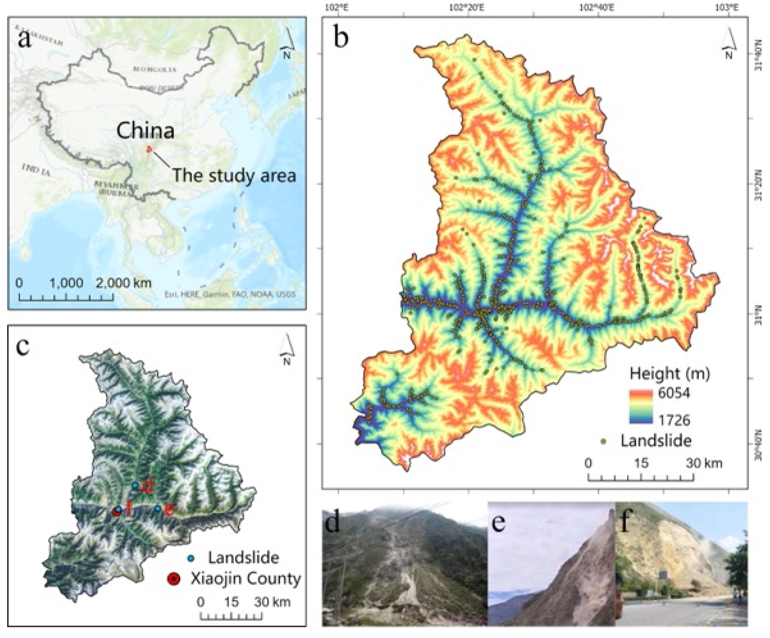
2.1. Study Area and Data

2.1.1. Study Area

Xiaojin County is located between longitudes 102°01′ E to 102°59′ E and latitudes 30°35′ N to 31°43′ N in part of the Aba Tibetan and Qiang Autonomous Prefecture, Sichuan Province, China (Figure 1) Xiaojin County is in the plateau area covering about 5582 km², and its terrain is high in the northeast and low in the southwest. The average mountain ridge is about 4500 m with the Siguniang Mountain in the east, as high as 6250 m. The valley area is more than 3000 m and the vertical distance is 1500–2500 m.

Xiaojin County located in the alpine valley on the edge of the Qinghai-Tibet Plateau, clamped between the seismic activity zone of the Longmen Shan fault zone and the seismic activity zone of the Xian Shui river fault zone. During the Wenchuan Earthquake and the Lushan earthquake, a large number of geological disasters occurred in the study area, resulting in serious casualties and property losses [3]. The climate of the study area is a subtropical monsoon climate zone. The average annual rainfall is 613mm, and the rainfall period is mainly from June to September. The Fubian River and the Xiaojin River are the main rivers in this area. The length, multi-year average flow, and multi-year average annual runoff of the Fubian River and Xiaojin River are 83 km and 150 km, 37.43 m³/s and 103 m³/s, 2.9 billion m³ and 1.2 billion m³, respectively. It is worth mentioning that the drop of these two rivers is very large, reaching 1960 m and 2340 m, respectively.

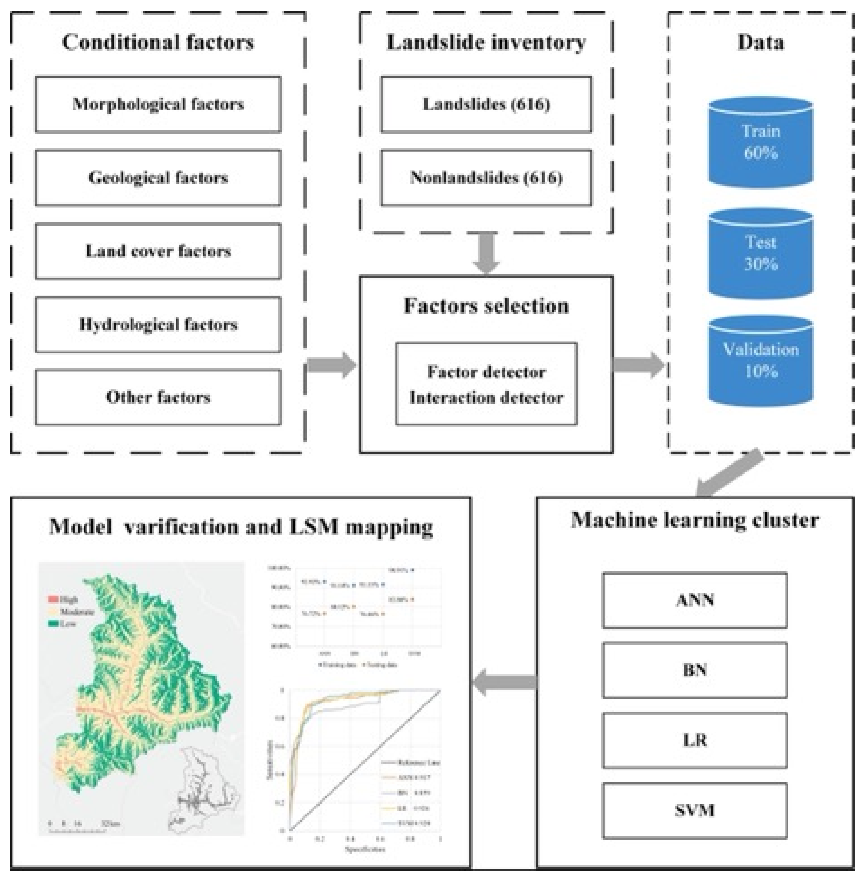
2.1.2. Landslide Inventory Map

In total, 616 landslides from 1949 to 2015 were obtained based on remote sensing image interpretation and field geological hazards survey by Sichuan Chuanjian Geotechnical Survey and Design Institute (http://www.sccjk.com/) (accessed on 22 December 2020) (Figure 1). These images were interpreted from the Resources satellite three (ZY-3) with 2.1 m ground pixel resolution. These interpretations and surveys are consistent with the adoption of the National Land Survey (http://www.mnr.gov.cn/) (accessed on 22 December 2020). This landslide inventory contains flow (debris flow, mudflow), fall (rockfall, debris/boulder fall), and slide (rock slide, gravel/sand/debris slide). These landslide types are defined by the new version of the Varnes classification system [27] (Figure 1d–f). Some areas in the study area are covered by glaciers and snow, which are indicated in white in the remote sensing image in Figure 1b. This study did not consider ice avalanches as a type of landslide.

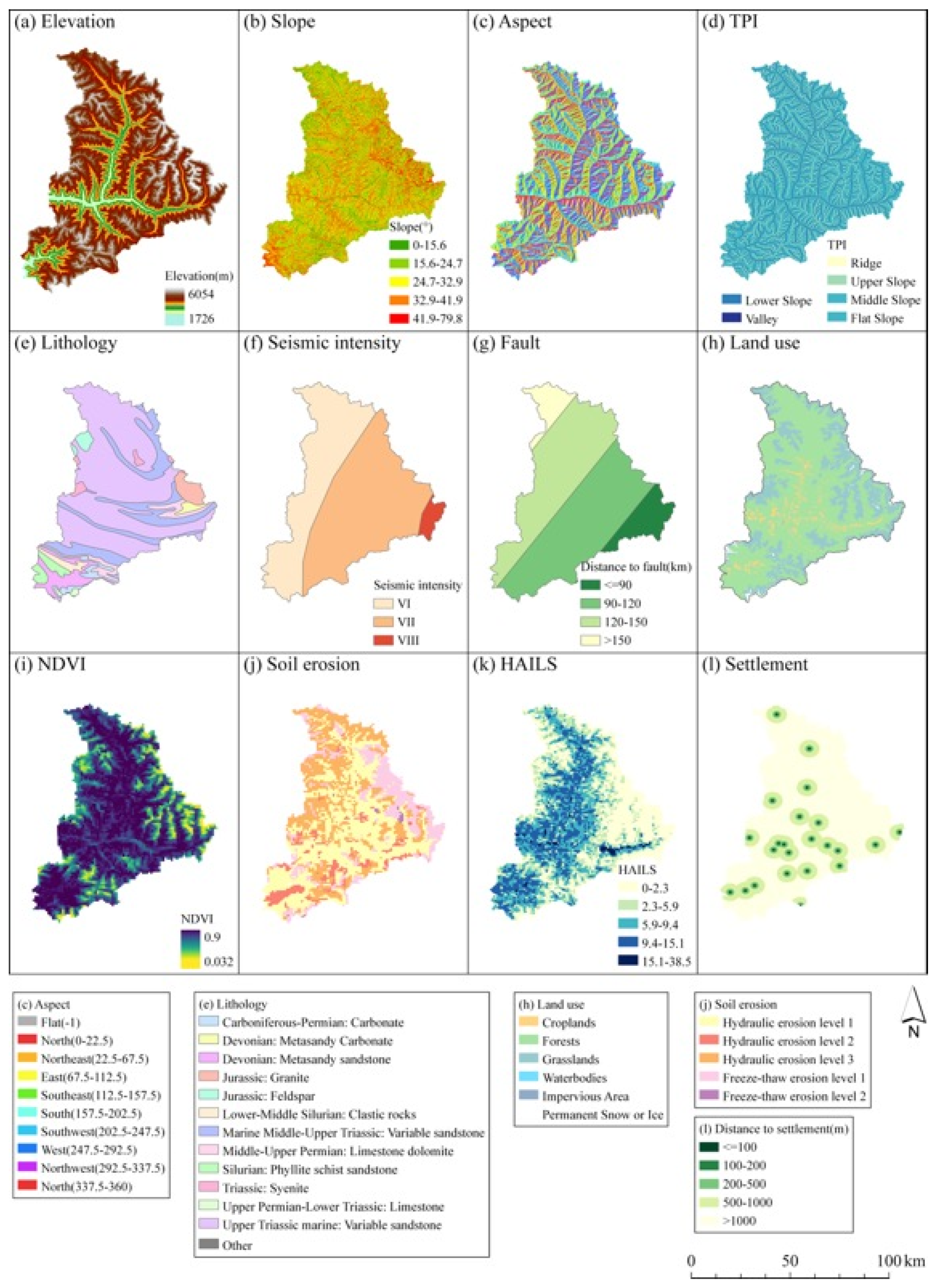
2.1.3. Conditional Factors

The selection of appropriate conditional factors is paramount in modeling [30]. Based on the geographical and environmental settings of the study area and literature [4,31], all 19 conditional factors have been selected and classified into five clusters: (i) morphological (6 variables), (ii) geological (3 variables), (iii) land cover (3 variables), (iv) hydrological (4 variables), and (v) other factors (3 variables) (

Table 1. The names, structures, and descriptions of conditional factors.

Cluster	Name	Data Description
Morphological	Elevation	Height above sea level
	Slope	Slope angle
	Aspect	Slope aspect
	Profile curve	Curvature along the slope
	Plan curve	Curvature perpendicular to slope
	TPI	Topographic position index
Geological	Lithology	Rock feature
	Seismic intensity	Magnitude of the earthquake
	Fault	Distance to fault zone
Land cover	Land use	Land use
	NDVI	Normalized Difference Vegetation Index
	Soil erosion	Hydraulic erosion and freeze-thaw erosion
Hydrological	Precipitation	Mean annual rainfall (1980–2010)
	River	Distance to river
	SPI	Stream power index
	TWI	Topographic wetness index, calculated by SAGA
Anthropogenic	HAILS	Human activity intensity of land surface
	Settlement	Distance to residential area
	Road	Distance to road

). All continuous variables were reclassified into five categories using the natural break method, while discrete variables were divided according to the characteristics of the data (Figure 2).

(i)

Morphological factors

Six morphometric factors were selected, including elevation, slope, aspect, profile curve, plan curve, and topographic position index (TPI). The elevation data was obtained from the ASTER GDEM V2.0 dataset distributed (spatial resolution of 30 m). Slope, aspect, profile curve, plan curve, and some relevant variables in the other clusters (i.e., TWI, SPI) were also derived from this dataset.

Elevation has a significant impact on the occurrence of landslides [10,32]. In this study area, most of the area is between 2000 and 4000 m above sea level and has large local elevation differences, which provide conditions for landslides to develop (Figure 2a). In general, hills with steep slopes are more prone to instability [33]. In this study area, 80% of slopes with slope angle among 20° to 40°, and the steepest slope angle is more than 70° (Figure 2b). Aspect mainly affects the stability of the slope mainly by affecting solar radiation and airflow (Figure 2c). Two different curvatures were morphometric variables which are profile and plan curvature. The profile curve affects the acceleration and deceleration of the flow, which in turn influences erosion and deposition. By contrast, the plan curve affects the convergence and dispersion of the flow. The TPI is a terrain parameter proposed by Andrew Weiss in 2001 to describe the terrain [34] (Figure 2d).

(ii)

Geological factors

Geological conditions are the controlling factors of landslide disasters [35]. This area was affected by tectonic activities of the Longmen Shan fault zone resulting in the deformation and formation of complex geological structures. Therefore, lithology, seismic intensity, and distance to fault were chosen as geological variables. The Longmen Shan Fault is located to the east outside the study area, so the distance to the fault increases progressively from east to west, as shown in Figure 2g. Geologically the strata in this area are mainly marine sediments of the Upper Triassic. The exposed sediments are mainly the Triassic and Jurassic strata. The lithology is mainly metamorphic sandstone and long granite. The engineering rock group is dominated by softer rock and hard rock, and the soft rock and hard rock are mixed in the small area of the south (Figure 2e). Seismic intensity indicates the intensity of the earthquake’s impact on the surface and engineering buildings. The seismic intensity in most parts of the county is VI and VII. In the east, the intensity is VIII (Figure 2f). The seismic intensity data is formulated under the national standard “China Earthquake Parameter Zoning Map” (GB18306-2001).

(iii)

Land cover factors

Land cover affects the stability of the ground and slopes [16,36]. The land cover cluster includes land use, NDVI, and soil erosion. The study area is covered by forests and grasslands, accounting for 67% and 27%, respectively (Figure 2h). Under the combined effect of climate and soil, the woods and grasses are not lush, and their positive effects on the stability of the slope are not strong [6]. The NDVI map can quantify the growth of green plants on the surface, which is closely related to the stability of the slope [37] (Figure 2i). Soil erosion is the result of interaction and mutual constraints of various factors in the geographical environment [38] (Figure 2j). The study area mainly has hydraulic erosion and freeze-thaw erosion, including 4 levels according to the general requirements of the People’s Republic of China industry-standard SL 190-96 "Classification Standard for Soil Erosion Classification".

(iv)

Hydrological factors

Precipitation, river, Stream power index (SPI), and Topographic wetness index (TWI) were selected as the hydrological factors. Water infiltration may reduce the stability of the slope, and continuous heavy rainfall can directly trigger landslides [39]. Due to its landlocked and plateau location, the study area does not receive much rainfall and river runoff is low. SPI measures the erosive force of water flow and has been used in different models [40]. TWI is a hypothetical measure of the cumulative amount of index water flow at any point in the basin, the TWI was calculated by SAGA-GIS software (http://saga-gis.org) (accessed on 22 December 2020) [32].

(v)

Anthropogenic factors

The anthropogenic factors include Human activity intensity of land surface (HAILS), settlement, and road. The HAILS is a synthesis index for describing the effect and influence of land surface [41,42] (Figure 2k). The HAILS is the extent to which humans use, rebuild, and develop the natural surface of the land. As a new composite index, it has been applied in some studies and achieved good results [43]. The HAILS is calculated by dividing the construction land equivalent by the total area of the region [42]. The existence of settlements and the construction of roads are the most active human activities on natural slopes. The multi-buffer distance to the settlement and the road were used to quantify the impact of the settlement and road, respectively (Figure 2l).

2.2. Methods

This workflow mainly consists of conditional factor selection, LSM modeling, and model validation (Figure 3). First, the conditional factor selection includes the Factor-detector and Interaction-detector methods in the GeoDetector. The GeoDetector software is freely available from http://www.geodetector.cn/ (accessed on 22 December 2020). Then, a machine learning cluster with four algorithms was used to model LSM. Finally, prediction accuracy and the ROC curves were used to validate the results.

Before factor selection and model construction, the study area was divided into regular grids with a spatial resolution of 60 m. The choice of grid size is determined by the computational efficiency, in addition, the choice of 60 m can effectively avoid the disorderly cutting of the grid for the factors (most factors have a spatial resolution of 30 m). Consequently, 1,709,680 mapping units are obtained. This makes the grid and the factors have a good correspondence with the unit of conditional factors. The number of landslide points in each mapping unit is calculated to obtain the y-variable for the GeoDetector. A total of 616 landslide points is distributed among 616 mapping units, making the y-variable a binary variable. The 19 discrete x-variable layers and y-variable layers are subjected to spatial overlay analysis. And each obtained unit has attributes of each conditional factor.

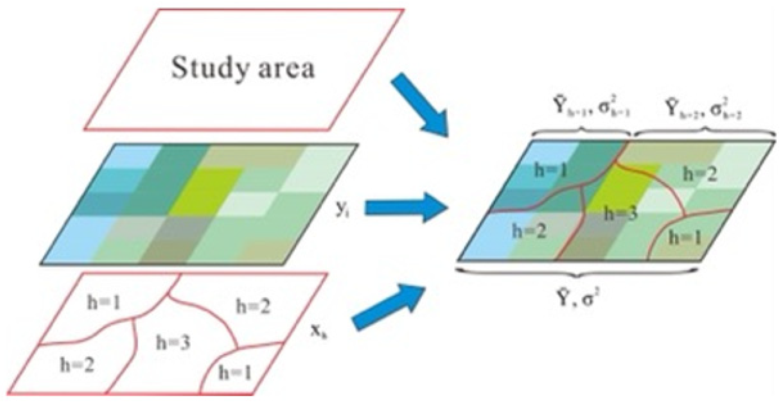
2.2.1. Conditional Factor Selection

Choosing the suitable conditional factor and defining the effective redundant factors affect the performance of LSM mapping. The effects of factors are mainly individual and interactive, both of which are extremely important, yet most current studies do not focus on interactive effects. The GeoDetector method can calculate the effects of factors individually as well as to detect interactions between factors [44]. This method was first applied in neural tube defects [45]. Subsequently, GeoDetector was applied in many areas, including landslide hazards [46], land use [47], regional economy [48], and ecosystem [49].

The core hypothesis of GeoDetector is that if an independent variable affects a dependent variable, the spatial distributions of the independent variable and the dependent variable should tend to be consistent [44,45,50]. The principle of GeoDetector is illustrated in Figure 4. The Factor-detector can detect how much factor X explains the spatial distribution of the variable Y. The principle of Factor-detector is as follows:

$$q=1 - \frac{{{\displaystyle \sum }}_{\mathrm{h}=1}^{\mathrm{L}}{N}_{\mathrm{h}}{\sigma }_{\mathrm{h}}^2}{{N\sigma }^2}$$

(1)

where q value is the metric for factor X; L is strata (category) of X or Y; N_h and N are the number of strata h and global strata, respectively; ${\sigma }_{\mathrm{h}}^2$ and ${\sigma }^2$ are the variances of the dependent variable Y of strata h and the variance of the entire area, respectively.

Interaction-detector can be used to identify interactions between conditional variables Xs. It can evaluate whether the factors X₁ and X₂ will change the explanatory power of the dependent variable Y when they work together, or the influence of these factors on $\gamma$ is independent. In the method of evaluation, the q values of X₁ and X₂ for Y: ${q\left(Y\right|X}_1)$ and ${q\left(Y\right|X}_2)$ are first calculated separately. Then, X₁ and X₂ are overlaid to form a new strata, and calculating the value of $X_1\cap X_2$ for Y: ${q\left(Y\right|X}_1\cap X_2)$. Finally, the value of ${q\left(Y\right|X}_1)$, ${q\left(Y\right|X}_2)$, and ${q\left(Y\right|X}_1\cap X_2)$ are compared to judge the interaction.

2.2.2. Machine Learning Cluster

The machine learning cluster contains four typical MLTs: artificial neural networks, Bayesian network, logistic regression, and support vector machines. The idea of the machine learning cluster comes from automatic machine learning (AutoML). AutoML can be seen as designing a series of advanced control systems to operate the machine learning model so that the model can automatically learn the appropriate parameters and configurations without manual intervention [51,52].

The dataset for the modeling consists of the positive and the negative sample. The positive sample set includes 616 disaster points of the field survey. The negative sample set is used to maintain the balance of the data samples, which are 100 m away from the known landslide points (positive samples). A sample set consisting of 616 non-landslide points is randomly selected. In total, 1232 points are randomly divided into three sample data groups. 60% of the sample data is set as the training dataset, 30% of the sample data is set as the testing dataset, and the other 10% of the data is the validation dataset.

(i)

Artificial neural network (ANN)

Artificial neural networks are generic non-linear function approximators that have been widely used in landslide susceptibility modeling in recent years [53]. ANN not only has the common characteristics of general non-linear systems, but also has its characteristics, such as high dimensionality, the extensive interconnection between neurons, and self-adaptation [17,54]. A standard neural network consists of many simple and connected processors called neurons, each producing a sequence of real-valued activations. Such systems learn to perform tasks by considering examples, generally without being programmed with task-specific rules.

MLP (multilayer perceptron) and RBF (radial basis function) are two common network structures of ANN. An MLP allows for more complex relationships at the possible cost of increasing the training and scoring time. An RBF may have lower training and scoring times, at the possible cost of reduced predictive power compared to the MLP. The classification ability and training time of the MLP and the RBF on the data in this study were examined, the hidden layers were set to be computed automatically, boosting algorithm was used to enhance the accuracy of the models. The results show that the time cost for the MLP and the RBF are about the same: 156 s and 139 s, respectively. However, the accuracy of MLP is 92.9%, which is higher than that of RBF at 85.5%. Thus the MLP was significantly better than the RBF, the MLP was selected for the experiments.

(ii)

Bayesian network (BN)

A Bayesian network is a graphical model that shows variables (usually called nodes) and their probabilities in a data set, as well as conditions and independence between these variables. This technique has been successfully applied for assessing landslide susceptibility [55,56]. In this study, the Naive Bayes Model (NB) is used to create a Bayesian network model. The likelihood ratio is used as an independent test. The joint probability of Bayesian networks can be expressed as the product of the edge probability of each node:

$$P(L,M,N)=P\left(L\right)\text{×}P\left(M\right|L\left)\text{×}P\right(N|L,M)$$

(2)

where P(L) is the prior probability that is the conditional probability without parent nodes, $P\left(M\right|L)$ is the conditional probability that is the occurrence probability of M under the L conditions, $P\left(N\right|L,M)$ is the conditional probability that is the occurrence probability of N under the L and M conditions.

(iii)

Logistic regression (LR)

Logistic regression is a statistical model that uses a logistic function to model a binary dependent variable and multiple independent variables. Its working principle is to construct a regression relationship between binary variables and independent variables for judging the probability of an event under certain conditions. If a landslide event is considered as a two-category event (occurs or does not), the binomial logistic regression model is very suitable for landslide susceptibility modeling [30,57]. The principle equation governing the LR model is as follows:

$$P(Y=1)=\frac{{exp(\alpha +\beta }_1{x}_1{+\beta }_2{x}_2+\cdots {+\beta }_n{x}_n)}{{1+exp(\alpha +\beta }_1{x}_1{+\beta }_2{x}_2+\cdots {+\beta }_n{x}_n)}$$

(3)

where $\alpha$ is a constant term, ${\mathrm{x}}_1{,\mathrm{x}}_2{\text{…}\mathrm{x}}_{\mathrm{n}}$ are independent variables, and ${\beta }_1, {\beta }_2\dots {\beta }_n$ are the regression coefficients to be determined. The output probability, P_i value, ranges from 0 to 1, where 0 means that the probability of a landslide in the mapping unit i is 0, and 1 means that the probability of a landslide in the mapping unit i is 1.

(iv)

Support Vector Machine (SVM)

SVM is a generalized linear classifier that classifies data in a binary manner based on supervised learning. Its basic model is a linear classifier with the largest interval defined in the feature space. The basic idea of SVM learning is to solve the separation hyperplane that can correctly divide the training data set and has the largest geometric interval. SVM also includes kernel techniques, which makes it essentially a non-linear classifier. The prediction accuracy of an SVM is affected by the selection of the kernel functions such as sigmoid, polynomial, linear, and radial basis function (RBF). The kernel function of RBF, which is defined based on the Euclidean Distance, is the most used kernel function for landslide susceptibility assessment. The principal equation governing the RBF is as follows:

$${K(x}_{\mathrm{i}},x_{\mathrm{j}})=exp\left(-\frac{\Vert x_{\mathrm{i}}-x_{\mathrm{j}}\Vert }{{2\mathsf{\sigma }}^2}\right)$$

(4)

where with $\mathsf{\sigma }>0$, the parameter which determines the width of the RBF, $k\left(.,.\right)$ is a kernel function, $x_{\mathrm{i}}$, $x_{\mathrm{j}}$ are the vectors of the ith and jth training sample vectors, respectively.

2.2.3. Verification

In the current study, the predictive accuracy, the ROC curve method, and the seed cell area index (SCAI) method are for verification and comparison of the models. Predictive accuracy was used to quantitatively evaluate the accuracy of 0-value and 1-value predictions and the overall predictive accuracy. The ROC curve is a graph based on the sensitivity (also known as the true positive rate) and 1−specificity (also known as the false positive rate) with various cut-off thresholds. It is used to assess the prediction accuracy quantitatively [58]. The area under the ROC curves (AUC) can be considered as the statistical summary of the overall performance. The AUC is commonly recognized as the most useful accuracy statistic for landslide susceptibility modeling. SCAI was the ratio of the percentage area of each susceptibility class to the percentage of landslides that occur in each class [59]. Compared to predictive accuracy and ROC, SCAI can provide more details about the classification results of models.

3. Results

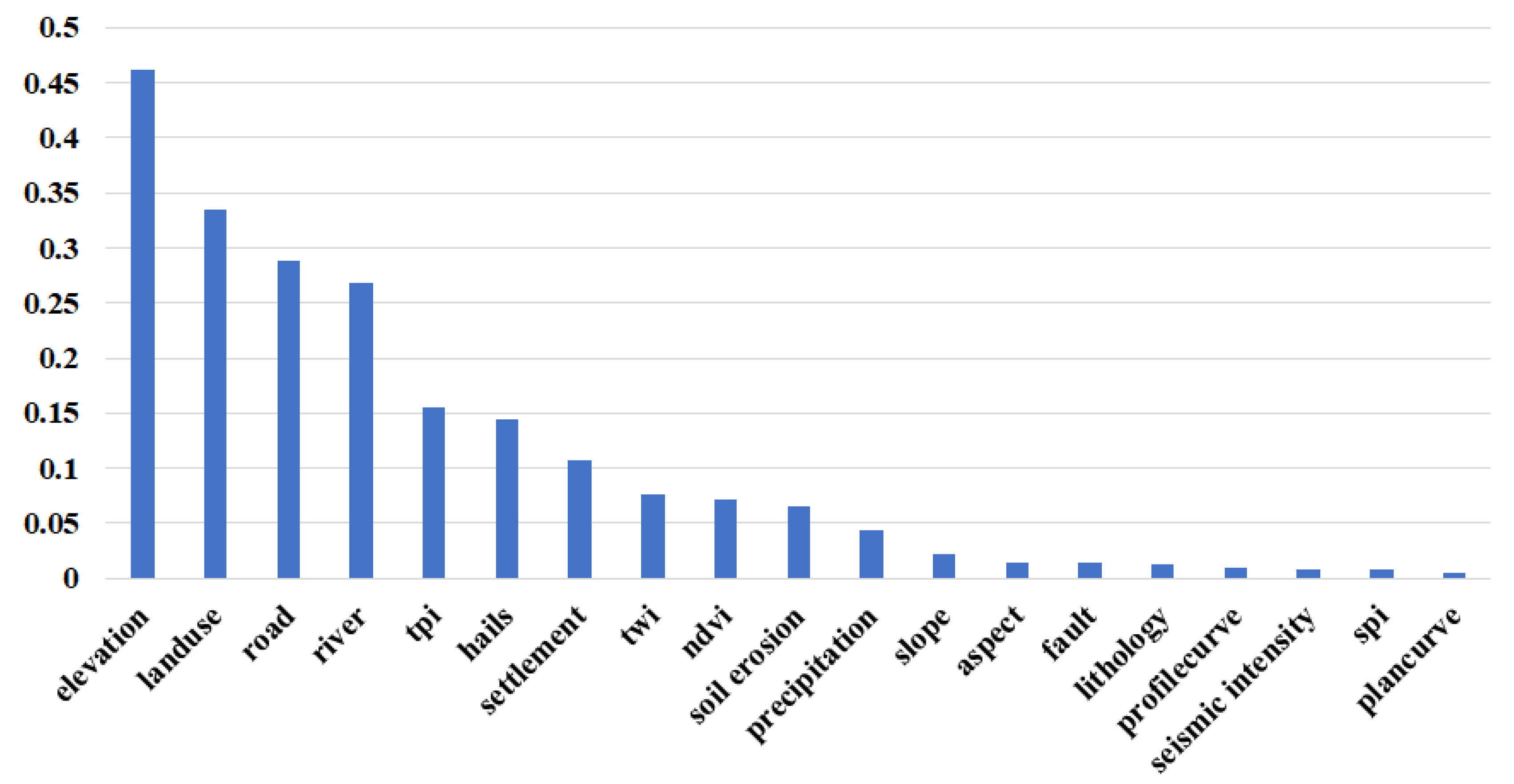
3.1. Results of Conditional Select

The results of the spatial overlay analysis are imported into GeoDetector for calculation, and the q value of each conditional factor is obtained. At the same time, the p-value of each conditional factor is also calculated. The p-value is a parameter used to determine the results of a hypothesis test. The calculation results of Factor-detector and Interaction-detector are as shown in Figure 5 and Figure 6, respectively.

The elevation is the most important factor (with q of 0.46), which is followed by land use (0.33), road (0.29), and river (0.27). And the q of plan curve, seismic density, SPI, and profile curve are all less than 0.01, they are considered redundant factors [44]. Besides, the p-values for both TWI and profile curve are greater than 0.05, and thus the results are not statistically significant. As a result, the plan curve, seismic density, SPI, profile curve, and TWI should be eliminated. However, the result of the Interaction-detector provides additional information and insights beyond the above results. We can clearly see that seismic intensity plays a positive role in the interaction with other factors, as evidenced by the nonlinear enhancement of the cross-effects with each of the factors, while other factors do not have such a strong effect. So, we tried to keep the seismic intensity and remove the other four factors.

To test whether the decision to remove the redundant factor was correct, we constructed a simple random forest model and used Mean Absolute Error (MAE) to evaluate the utility of the removal. MAE is a commonly used measure of the usefulness of factor deletion, which represents the mean of the absolute value of the error between the observed and true values. The smaller its value, the better the performance of the model. Random forest models have good generalization capabilities and are often used in such tests. In this work, the random forest model was constructed using scikit-learn with n_estimators set to 100, random_state set to 0, and all other parameters left as default. The results showed that the MAE was 0.420 with all 19 factors retained, 0.395 with five factors (plan curve, seismic density, SPI, profile curve, and TWI) removed, and only 0.391 with four factors (plan curve, SPI, profile curve, and TWI) removed. Such results demonstrate that GeoDetector is effective for factor screening. Therefore, the conditional factor dataset with no redundant factors was used for machine learning modeling.

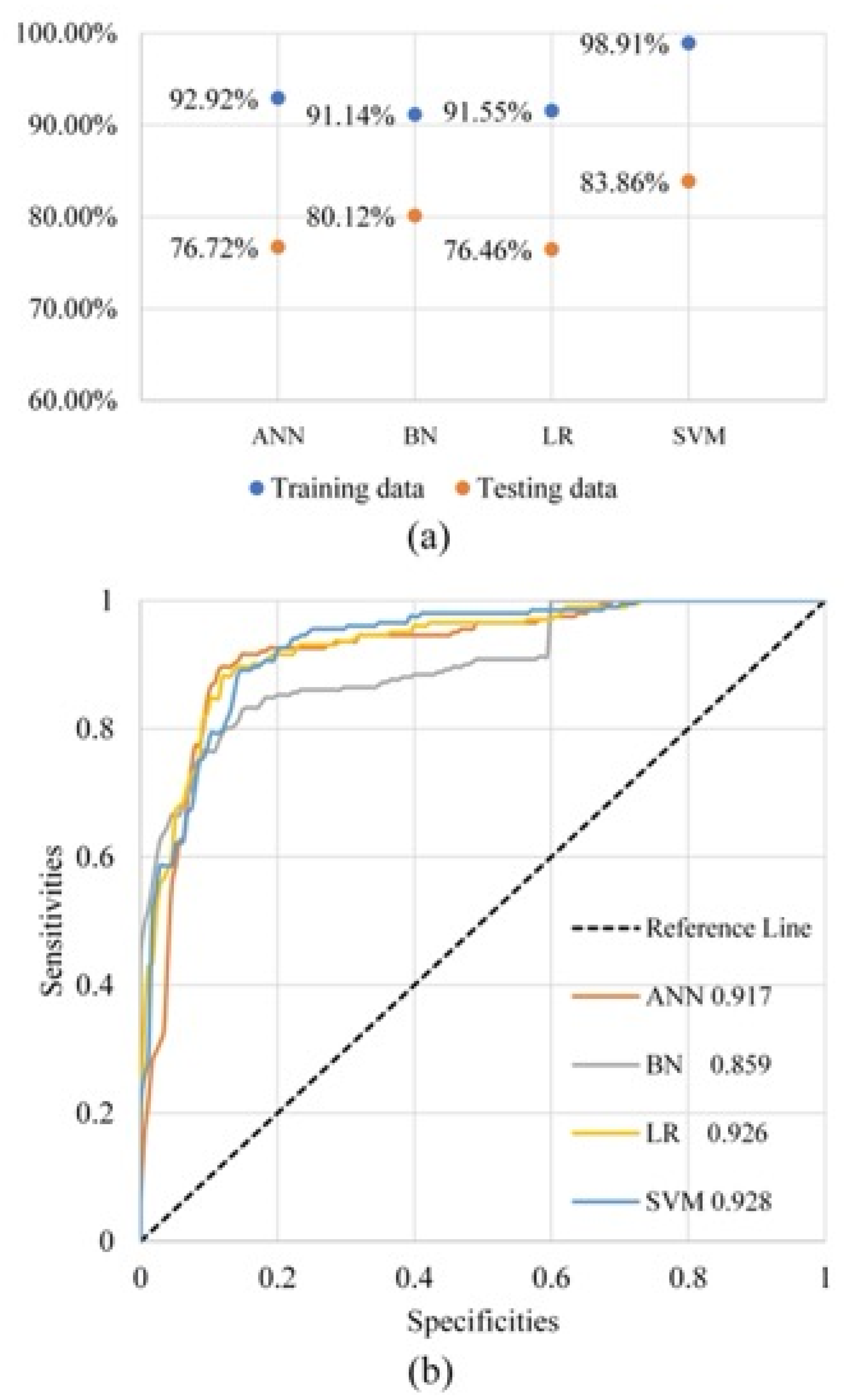
3.2. Accuracy Assessment of the Machine Learning Cluster

Verification and comparison of the model included prediction accuracy, the ROC curve, and SCAI. Figure 7 shows the prediction accuracy and the ROC curve of the machine learning cluster with training data and testing data. The results of SCAI are shown in

Table 2. The densities of landslide occurrence (SCAI) for ANN, BN, LR, and SVM models.

Model	Class	Pixel Number	Area (%)	Number of Landslides	Landslides (%)	SCAI
ANN	High	140,711	8.23	317	51.46	0.16
	Moderate	728,149	42.59	228	37.01	1.15
	Low	840,820	49.18	71	11.52	4.27
BN	High	193,365	11.31	258	41.88	0.27
	Moderate	661,817	38.71	263	42.69	0.91
	Low	854,498	49.98	95	15.42	3.24
LR	High	135,236	7.91	325	52.76	0.15
	Moderate	689,856	40.35	224	36.36	1.11
	Low	884,588	51.74	67	10.88	4.75
SVM	High	103,094	6.03	375	60.87	0.09
	Moderate	641,472	37.52	197	31.98	1.17
	Low	965,114	56.45	44	7.14	7.91

.

For the predictive accuracy of four MLTs, all models performed well in the training set, exceeding 90%, and SVM even reached over 98%. While for the testing data, SVM has the best performance with 83.86%, and no other model exceeds 80.5%. For the AUC, the BN has the weakest performance, with a score of only 85.9%. While the other three algorithms performed similarly and SVM still had the highest value. The results of SCAI showed that the classes were divided with high precision in four models (Table 2). High susceptibility classes have very low SCAI values (<1) in all models, which indicates the presence of many historical landslides in high susceptibility areas. And low susceptibility classes have high SCAI values (>3). Among them, the SCAI value of SVM is more prominent compared to other models: the lowest value of the high susceptibility class. All the way, the SVM has the best performance under three verification indicators. Therefore, the machine learning cluster automatically selects SVM as the optimal model for calculation and output the results.

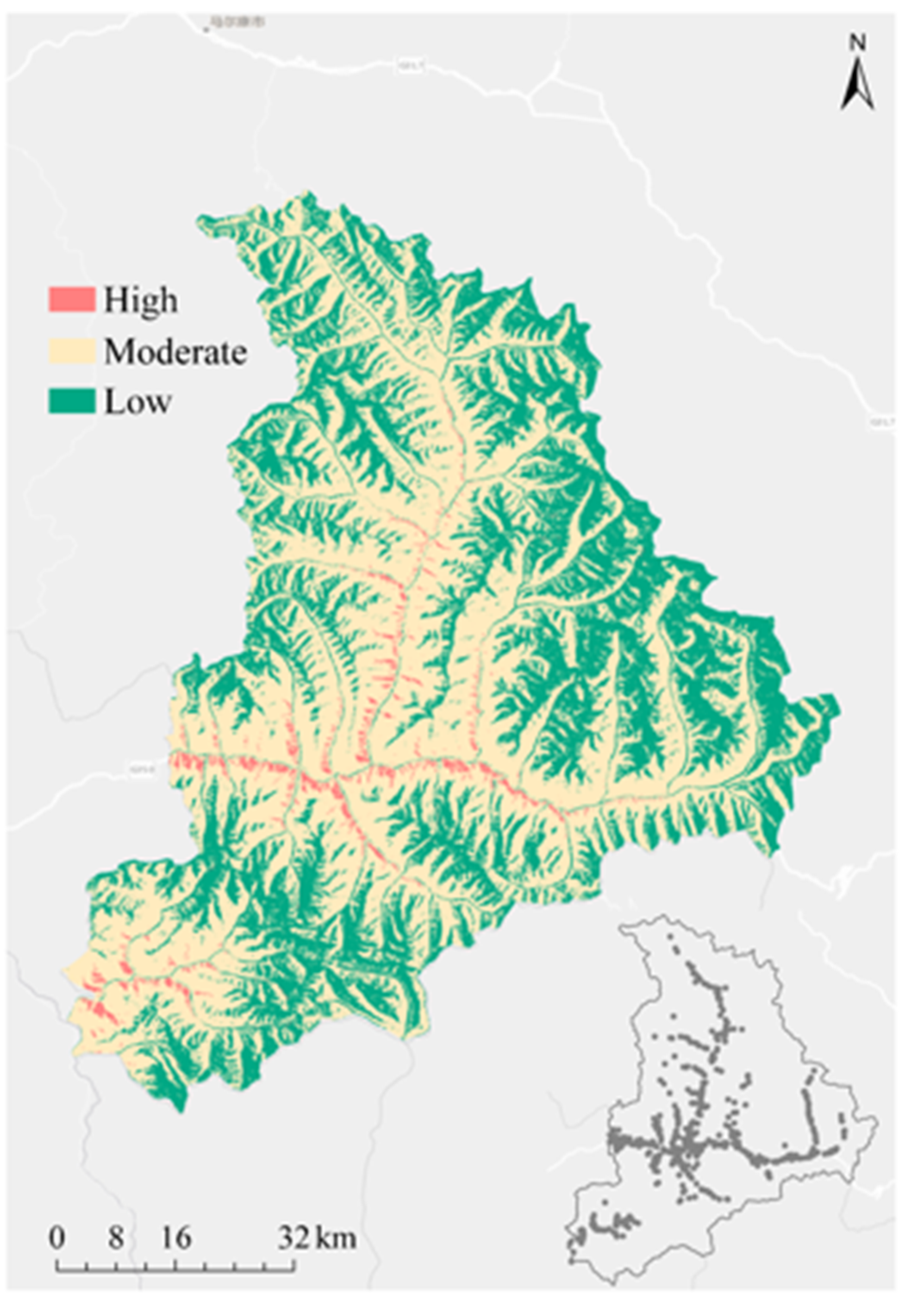
3.3. Landslide Susceptibility Mapping

The LSM was prepared by generating landslide susceptibility indices (LSIs) and reclassifying the class. The LSI was calculated based on the trained machine learning cluster. Using the natural breaks method, the LSM was reclassified into three susceptibility classes: high, moderate, and low (Figure 8). The reason for classifying the susceptibility into five or more classes is that if they were divided into five or more classes, the high susceptibility areas would occupy only a very small share and thus be difficult to show on the map. As shown in Figure 8, high, moderate, and low susceptibility areas have distinct zoning characteristics. The proportion of areas occupied by high, moderate, and low areas is 6.03%, 37.52%, and 56.45%, respectively, while the proportion of landslides they correspond to is 60.87%, 31.98%, and 7.14%, respectively. The high susceptibility areas were concentrated in urban areas and in areas where previous disasters had occurred, which were also concentrated near roads and rivers.

4. Discussion

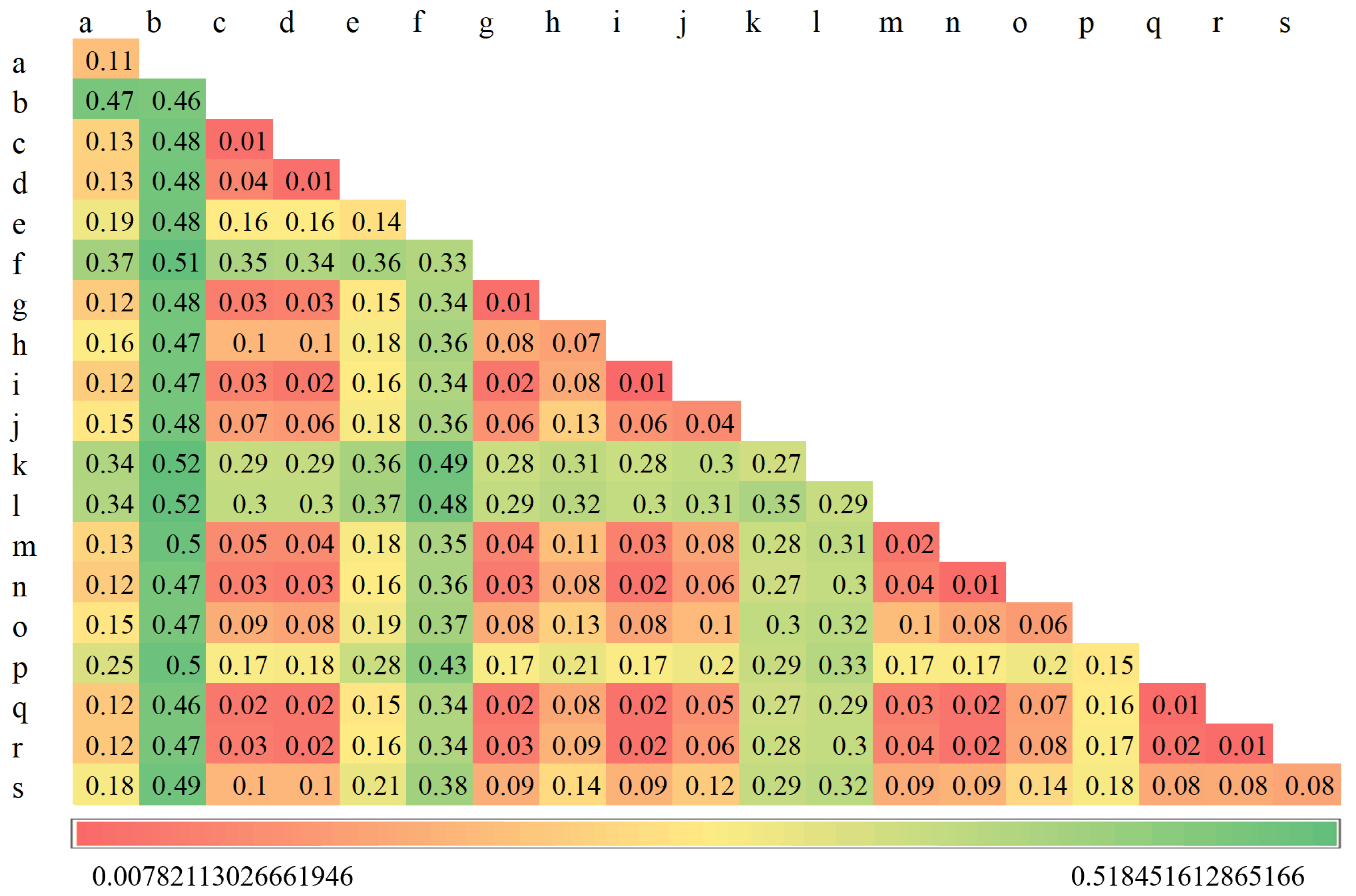
4.1. Factor-Detector and Interaction-Detector

As a result of the common effect between natural processes and human activities, landslides are largely related to natural environmental conditions. And the susceptibility of landslides should tightly grasp this objective fact. Geographers, geologists, and ecologists have discovered and created many measures to characterize the various geographic environmental conditions and the impact of human activities associated with landslides. These conditions are not universal but different in different places and even at different times. The selection of landslide conditional factors and defining the effective redundant factors for the study area is critical. One strategy is to first prepare comprehensive conditional factors, including geology, hydrology, human activities, then effectively screen out the conditional factors and remove redundant factors.

The results of the Factor-detector show that elevation is the most important factor and this result is consistent with many studies [60]. When the altitude in an area varies hugely, elevation becomes an important factor affecting the occurrence of landslides. The results also show the importance of three human-related variables: roads, HAILS, and settlements (Figure 5). According to the spatial distribution of landslide data and the location of roads and residential areas, anthropogenic activities in this area have a strong effect on landslides. In other studies, factors related to anthropogenic human activities are considered to have a significant effect on the occurrence of landslides [61]. In mountainous areas, the construction of roads may cut slopes that were stable, thus destroying the original balance. The closer to the road the more severely damaged the slope is, and the greater the likelihood of landslides. Moreover, poorly constructed roads pose more serious hazards to slopes than well-constructed roads under the same conditions. The spatial heterogeneity of human activities is much greater than the natural environmental conditions. The distribution of landslides in the study area fits this heterogeneity. That is the reason why human activities can greatly affect the distribution of landslides.

The slope and aspect did not play a huge role in affecting the occurrence of landslides (Figure 5). Slope and aspect are generally considered important factors in LSM. However, many studies believe that slope and aspect are not very important, which are consistent with the results of our study [21,62]. In this study area, landslides are mainly distributed in areas with small slopes. This distribution makes the model believe that the occurrence of landslides does not change when the slope changes within a larger range, so the slope is considered to have a small contribution. Locally, it is the road, not the slope or aspect disrupting the original slope shape and the landslide. Seismic density does not score high in the Factor-detector’s result but very active in Interaction-detector. Its interaction with most of the factors is a non-linear enhancement. Because it has a fixed value in the area of dozens of kilometers, that is, the same seismic in a place and another place ten-kilometers away from it. This leads to the factor provide little contribution because of the weak spatial heterogeneity.

Interaction-detector can calculate the interaction between different factors (Figure 6). In this study, Interaction-detector’s results show a high degree of consistency with the results of Factor-detector. Furthermore, the Interaction-detector can find the reciprocal action among factors that the Factor-detection ignores. In this regard, the role of the Interactive-detector is highlighted because it emphasizes the interaction between the factors. Strong earthquake intensity does not induce landslides in places where the slope angle is small, but it greatly induces landslides in places where the slope angle is large. Similarly, rivers are difficult to cause surface deformation in the forest, while they can easily cause instability on slopes near the highway.

Combining the results of Factor-detector and Interaction-detector, we considered TWI, profile curve, SPI, and plan curve as redundant factors. By comparing the effects before and after the use of the Factor-detector and the Interaction-detector, it is easy to see a significant change in the MAE values. When the Factor-detector was used, the MAE decreases from 0.420 to 0.395, and when the results of the Interaction-detector are considered on this basis, the MAE decreased to 0.391. These results demonstrated the superiority of the method used in this work.

4.2. Machine Learning Cluster Performance

When the input data enters the machine learning cluster, it automatically selects the most suitable model according to the model performance. In this case, SVM had the best performance in this study area and was selected for landslide susceptibility mapping. The model performance was evaluated by calculating the prediction accuracy, ROC, and SCAI statistics. The SCAI shows that high susceptibility classes have low SCAI values with less than 1, which means all four models have acceptable results. The prediction accuracy of the training dataset and testing dataset of SVM are 98.91% and 83.86%, respectively. The prediction accuracy of the other three models is at least 3% lower. Furthermore, the AUC of SVM is also higher than other models with 0.928 in the testing dataset. In the case of the same input data, different models perform differently. On the one hand, because the structure of the model itself is different, the classification criteria for the data are also different. On the other hand, because different factors play different roles in different models, that is to say, factors that have a low contribution in a given model may be useful for another and have a significant influence on the model. This also shows that for a certain study area, it is reasonable to compare multiple models and select the most appropriate one. Overall, it was observed that SVM has the best performance in the machine learning cluster, so the cluster choose SVM as the final output algorithm, and this result is matched with previous work [63]. SVM is an efficient algorithm for partitioning the hyperplane of binary data, which solves the problem of classifying binary data by finding the minimum support vector between the data and the hyperplane. This feature allows the SVM to be advantageous in landslide susceptibility assessment where landslides are represented as binary data.

A traditional method often chooses only one model for training and prediction, which may ignore other potentially better models. In this study, we selected several typical MLTs for processing landslides and conditional factors and finally obtained the LSM of the study area. The results of the machine learning cluster indicate that clustering is a good solution to the model selection and LSM.

4.3. New Contributions and Prospect of Model

As previously mentioned, machine learning methods have been widely applied to LSM. Pham et al. [61] proposed a new hybrid model of sequential minimal optimization and SVM (SMOSVM) for accurate LSM. The results showed that the new model (AUC = 0.824) had a better performance than SVM and naive Bayes trees (NBT). The present study has similar findings to this study, indicating that SVM is an excellent and continuously optimizable method. Yang et al. [46] proposed a new method based on the GeoDetector and spatial LR model, the prediction accuracy of the new method was found to be 86.1%, which is an 11.9% improvement over the traditional LR model. Compared with [46], our study digs deeper into the function of factor interaction of GeoDetector and applies this function to landslide impact factor selection. This approach provides a new perspective to the problem of factor selection in broader earth science. Dou et al. [62] examined and evaluated the predictive capability of SVM hybrid ensemble ML algorithms, i.e., the bagging, boosting, and stacking. The results showed that the SVM-boosting model outperformed SVM-Stacking, SVM, and SVM-Bagging, which indicated that ensemble learning does not necessarily have an enhancing effect on an algorithm. This further suggests that the selection of an appropriate model is critical for LSM, which is consistent with our study. Our study proposes a simple and effective approach for LSM: putting multiple typical machine learning methods into a cluster and selecting the best model in the cluster for different study areas.

In conclusion, compared with the above studies, the new contributions of this study are (1) a factor selection method based on Factor-detector and Interactive-detector, and (2) a solution for machine learning model selection.

5. Conclusions

This study aimed to improve the reliability of LSM by using the GeoDetector and a machine learning cluster. For this reason, 616 landslides and 19 landslides conditional factors in Xiaojin County were prepared in GIS. Using Factor-detector and Interactive-detector to quantitatively analyze the individual and interactive effects of landslide conditional factors is an effective and reasonable approach. This approach provides an effective way to identify and eliminate redundant factors, the results show that plan curve, SPI, profile curve, and TWI are redundant factors. We designed a random forest model to test the effect of removing the redundant factors, and the MAE reduced from 0.420 to 0.391 after the removal, indicating the superiority of the GeoDetector. The machine learning cluster contains a variety of MLTs, and can automatically select the best model. In this case, the selected SVM had a prediction accuracy of 83.86% and an AUC value of 0.928. Thus, GeoDetector and the machine learning cluster were combined to make a landslide susceptibility map of the study area are very feasible. These approaches provide a general solution that accurately selects conditional factors and machine learning models, which could enhance the reliability of landslide susceptibility maps.

References

1. Gariano, S.L.; Guzzetti, F. Landslides in a changing climate. Earth Sci. Rev. 2016, 162, 227–252. [Google Scholar] [CrossRef] [Green Version]
2. Paranunzio, R.; Chiarle, M.; Laio, F.; Nigrelli, G.; Turconi, L.; Luino, F. New insights in the relation between climate and slope failures at high-elevation sites. Theor. Appl. Climatol. 2019, 137, 1765–1784. [Google Scholar] [CrossRef]
3. Fan, X.; Scaringi, G.; Korup, O.; West, A.J.; van Westen, C.J.; Tanyas, H.; Hovius, N.; Hales, T.C.; Jibson, R.W.; Allstadt, K.E.; et al. Earthquake-Induced Chains of Geologic Hazards: Patterns, Mechanisms, and Impacts. Rev. Geophys. 2019, 57, 421–503. [Google Scholar] [CrossRef] [Green Version]
4. Lin, Q.; Wang, Y. Spatial and temporal analysis of a fatal landslide inventory in China from 1950 to 2016. Landslides 2018, 15, 2357–2372. [Google Scholar] [CrossRef]
5. Lee, S.; Talib, J.A. Probabilistic landslide susceptibility and factor effect analysis. Environ. Geol. 2005, 47, 982–990. [Google Scholar] [CrossRef]
6. Van Westen, C.J.; Castellanos, E.; Kuriakose, S.L. Spatial data for landslide susceptibility, hazard, and vulnerability assessment: An overview. Eng. Geol. 2008, 102, 112–131. [Google Scholar] [CrossRef]
7. Reichenbach, P.; Rossi, M.; Malamud, B.D.; Mihir, M.; Guzzetti, F. A review of statistically-based landslide susceptibility models. Earth Sci. Rev. 2018, 180, 60–91. [Google Scholar] [CrossRef]
8. Budimir, M.E.A.; Atkinson, P.M.; Lewis, H.G. A systematic review of landslide probability mapping using logistic regression. Landslides 2015, 12, 419–436. [Google Scholar] [CrossRef] [Green Version]
9. Đurić, U.; Marjanović, M.; Radić, Z.; Abolmasov, B. Machine learning based landslide assessment of the Belgrade metropolitan area: Pixel resolution effects and a cross-scaling concept. Eng. Geol. 2019, 256, 23–38. [Google Scholar] [CrossRef]
10. Lee, J.H.; Sameen, M.I.; Pradhan, B.; Park, H.J. Modeling landslide susceptibility in data-scarce environments using optimized data mining and statistical methods. Geomorphology 2018, 303, 284–298. [Google Scholar] [CrossRef]
11. Brenning, A. Spatial prediction models for landslide hazards: Review, comparison and evaluation. Nat. Hazards Earth Syst. Sci. 2005, 5, 853–862. [Google Scholar] [CrossRef]
12. Lee, S.; Pradhan, B. Landslide hazard mapping at Selangor, Malaysia using frequency ratio and logistic regression models. Landslides 2007, 4, 33–41. [Google Scholar] [CrossRef]
13. Sharma, S.; Mahajan, A.K. A comparative assessment of information value, frequency ratio and analytical hierarchy process models for landslide susceptibility mapping of a Himalayan watershed, India. Bull. Eng. Geol. Environ. 2019, 78, 2431–2448. [Google Scholar] [CrossRef]
14. Ilia, I.; Tsangaratos, P. Applying weight of evidence method and sensitivity analysis to produce a landslide susceptibility map. Landslides 2016, 13, 379–397. [Google Scholar] [CrossRef]
15. Wang, Z.; Liu, Q.; Liu, Y. Mapping landslide susceptibility using machine learning algorithms and GIS: A case study in Shexian county, Anhui province, China. Symmetry 2020, 12, 1954. [Google Scholar] [CrossRef]
16. Lee, S. Application of likelihood ratio and logistic regression models to landslide susceptibility mapping using GIS. Environ. Manag. 2004, 34, 223–232. [Google Scholar] [CrossRef]
17. Harmouzi, H.; Nefeslioglu, H.A.; Rouai, M.; Sezer, E.A.; Dekayir, A.; Gokceoglu, C. Landslide susceptibility mapping of the Mediterranean coastal zone of Morocco between Oued Laou and El Jebha using artificial neural networks (ANN). Arab. J. Geosci. 2019, 12, 696–714. [Google Scholar] [CrossRef]
18. Moayedi, H.; Mehrabi, M.; Mosallanezhad, M.; Rashid, A.S.A.; Pradhan, B. Modification of landslide susceptibility mapping using optimized PSO-ANN technique. Eng. Comput. 2019, 35, 967–984. [Google Scholar] [CrossRef]
19. Tsangaratos, P.; Ilia, I. Comparison of a logistic regression and Naïve Bayes classifier in landslide susceptibility assessments: The influence of models complexity and training dataset size. Catena 2016, 145, 164–179. [Google Scholar] [CrossRef]
20. Raia, S.; Alvioli, M.; Rossi, M.; Baum, R.L.; Godt, J.W.; Guzzetti, F. Improving predictive power of physically based rainfall-induced shallow landslide models: A probabilistic approach. Geosci. Model Dev. Discuss. 2013, 6, 1367–1426. [Google Scholar] [CrossRef] [Green Version]
21. Yang, Y.; Yang, J.; Xu, C.; Xu, C.; Song, C. Local-scale landslide susceptibility mapping using the B-GeoSVC model. Landslides 2019, 16, 1301–1312. [Google Scholar] [CrossRef]
22. Xiao, L.; Zhang, Y.; Peng, G. Landslide susceptibility assessment using integrated deep learning algorithm along the china-nepal highway. Sensors 2018, 18. [Google Scholar] [CrossRef] [Green Version]
23. Huang, F.; Zhang, J.; Zhou, C.; Wang, Y.; Huang, J.; Zhu, L. A deep learning algorithm using a fully connected sparse autoencoder neural network for landslide susceptibility prediction. Landslides 2020, 17, 217–229. [Google Scholar] [CrossRef]
24. Pourghasemi, H.R.; Teimoori Yansari, Z.; Panagos, P.; Pradhan, B. Analysis and evaluation of landslide susceptibility: A review on articles published during 2005–2016 (periods of 2005–2012 and 2013–2016). Arab. J. Geosci. 2018, 11, 1–12. [Google Scholar] [CrossRef]
25. Youssef, A.M.; Pourghasemi, H.R.; Pourtaghi, Z.S.; Al-Katheeri, M.M. Landslide susceptibility mapping using random forest, boosted regression tree, classification and regression tree, and general linear models and comparison of their performance at Wadi Tayyah Basin, Asir Region, Saudi Arabia. Landslides 2016, 13, 839–856. [Google Scholar] [CrossRef]
26. Van Asch, T.W.J.; Buma, J.; Van Beek, L.P.H. A view on some hydrological triggering systems in landslides. Geomorphology 1999, 30, 25–32. [Google Scholar] [CrossRef]
27. Hungr, O.; Leroueil, S.; Picarelli, L. The Varnes classification of landslide types, an update. Landslides 2014, 11, 167–194. [Google Scholar] [CrossRef]
28. Jebur, M.N.; Pradhan, B.; Tehrany, M.S. Optimization of landslide conditioning factors using very high-resolution airborne laser scanning (LiDAR) data at catchment scale. Remote Sens. Environ. 2014, 152, 150–165. [Google Scholar] [CrossRef]
29. Chen, W.; Zhao, X.; Shahabi, H.; Shirzadi, A.; Khosravi, K.; Chai, H.; Zhang, S.; Zhang, L.; Ma, J.; Chen, Y.; et al. Spatial prediction of landslide susceptibility by combining evidential belief function, logistic regression and logistic model tree. Geocarto Int. 2019, 34, 1177–1201. [Google Scholar] [CrossRef]
30. Tehrany, M.S.; Jones, S.; Shabani, F.; Martínez-Álvarez, F.; Tien Bui, D. A novel ensemble modeling approach for the spatial prediction of tropical forest fire susceptibility using LogitBoost machine learning classifier and multi-source geospatial data. Theor. Appl. Climatol. 2019, 137, 637–653. [Google Scholar] [CrossRef]
31. Zhao, C.; Lu, Z. Remote sensing of landslides-A review. Remote Sens. 2018, 10, 279. [Google Scholar] [CrossRef] [Green Version]
32. Liu, L.; Li, S.; Li, X.; Jiang, Y.; Wei, W.; Wang, Z.; Bai, Y. An integrated approach for landslide susceptibility mapping by considering spatial correlation and fractal distribution of clustered landslide data. Landslides 2019, 16, 715–728. [Google Scholar] [CrossRef]
33. Pawluszek, K.; Borkowski, A. Impact of DEM-derived factors and analytical hierarchy process on landslide susceptibility mapping in the region of Rożnów Lake, Poland. Nat. Hazards 2017, 86, 919–952. [Google Scholar] [CrossRef] [Green Version]
34. Weiss, A.D. Topographic position and landforms analysis. In Proceedings of the ESRI User Conference, San Diego, CA, USA, 9–13 July 2001; Volume 64, pp. 227–245. Available online: http://www.jennessent.com/downloads/tpi-poster-tnc_18x22.pdf (accessed on 22 December 2020).
35. Chen, W.; Xie, X.; Wang, J.; Pradhan, B.; Hong, H.; Bui, D.T.; Duan, Z.; Ma, J. A comparative study of logistic model tree, random forest, and classification and regression tree models for spatial prediction of landslide susceptibility. Catena 2017, 151, 147–160. [Google Scholar] [CrossRef] [Green Version]
36. Beguerı, S. Changes in land cover and shallow landslide activity: A case study in the Spanish Pyrenees. Geomorphology 2006, 74, 196–206. [Google Scholar] [CrossRef] [Green Version]
37. Yang, W.; Wang, Y.; Sun, S.; Wang, Y.; Ma, C. Using Sentinel-2 time series to detect slope movement before the Jinsha River landslide. Landslides 2019, 16, 1313–1324. [Google Scholar] [CrossRef]
38. Guerra, A.J.T.; Fullen, M.A.; Do Carmo Oliveira Jorge, M.; Bezerra, J.F.R.; Shokr, M.S. Slope Processes, Mass Movement and Soil Erosion: A Review. Pedosphere 2017, 27, 27–41. [Google Scholar] [CrossRef]
39. Piciullo, L.; Calvello, M.; Cepeda, J.M. Territorial early warning systems for rainfall-induced landslides. Earth Sci. Rev. 2018, 179, 228–247. [Google Scholar] [CrossRef]
40. Kim, J.C.; Lee, S.; Jung, H.S.; Lee, S. Landslide susceptibility mapping using random forest and boosted tree models in Pyeong-Chang, Korea. Geocarto Int. 2018, 33, 1000–1015. [Google Scholar] [CrossRef]
41. Taalab, K.; Cheng, T.; Zhang, Y. Mapping landslide susceptibility and types using Random Forest. Big Earth Data 2018, 2, 159–178. [Google Scholar] [CrossRef]
42. Xu, Y.; Xu, X.; Tang, Q. Human activity intensity of land surface: Concept, methods and application in China. J. Geogr. Sci. 2016, 26, 1349–1361. [Google Scholar] [CrossRef]
43. Chi, Y.; Zheng, W.; Shi, H.; Sun, J.; Fu, Z. Spatial heterogeneity of estuarine wetland ecosystem health influenced by complex natural and anthropogenic factors. Sci. Total Environ. 2018, 634, 1445–1462. [Google Scholar] [CrossRef] [Green Version]
44. Wang, J.F.; Zhang, T.L.; Fu, B.J. A measure of spatial stratified heterogeneity. Ecol. Indic. 2016, 67, 250–256. [Google Scholar] [CrossRef]
45. Wang, J.F.; Li, X.H.; Christakos, G.; Liao, Y.L.; Zhang, T.; Gu, X.; Zheng, X.Y. Geographical detectors-based health risk assessment and its application in the neural tube defects study of the Heshun Region, China. Int. J. Geogr. Inf. Sci. 2010, 24, 107–127. [Google Scholar] [CrossRef]
46. Yang, J.; Song, C.; Yang, Y.; Xu, C.; Guo, F.; Xie, L. New method for landslide susceptibility mapping supported by spatial logistic regression and GeoDetector: A case study of Duwen Highway Basin, Sichuan Province, China. Geomorphology 2019, 324, 62–71. [Google Scholar] [CrossRef]
47. Ju, H.; Zhang, Z.; Zuo, L.; Wang, J.; Zhang, S.; Wang, X.; Zhao, X. Driving forces and their interactions of built-up land expansion based on the geographical detector—A case study of Beijing, China. Int. J. Geogr. Inf. Sci. 2016, 30, 2188–2207. [Google Scholar] [CrossRef]
48. Bai, L.; Jiang, L.; Yang, D.Y.; Liu, Y.B. Quantifying the spatial heterogeneity influences of natural and socioeconomic factors and their interactions on air pollution using the geographical detector method: A case study of the Yangtze River Economic Belt, China. J. Clean. Prod. 2019, 232, 692–704. [Google Scholar] [CrossRef]
49. Qi, X.; Si, Z.; Zhong, T.; Huang, X.; Crush, J. Spatial determinants of urban wet market vendor profit in Nanjing, China. Habitat Int. 2019, 94, 102064. [Google Scholar] [CrossRef]
50. Wang, J.F.; Hu, Y. Environmental health risk detection with GeogDetector. Environ. Model. Softw. 2012, 33, 114–115. [Google Scholar] [CrossRef]
51. Xavier-Júnior, J.C.; Freitas, A.A.; Ludermir, T.B.; Feitosa-Neto, A.; Barreto, C.A.S. An Evolutionary Algorithm for Automated Machine Learning Focusing on Classifier Ensembles: An improved algorithm and extended results. Theor. Comput. Sci. 2019, 805, 1–18. [Google Scholar] [CrossRef]
52. Waring, J.; Lindvall, C.; Umeton, R. Arti fi cial Intelligence in Medicine Automated machine learning: Review of the state-of-the-art and opportunities for healthcare. Artif. Intell. Med. 2020, 104, 101822. [Google Scholar] [CrossRef]
53. Poudyal, C.P.; Chang, C.; Oh, H.J.; Lee, S. Landslide susceptibility maps comparing frequency ratio and artificial neural networks: A case study from the Nepal Himalaya. Environ. Earth Sci. 2010, 61, 1049–1064. [Google Scholar] [CrossRef]
54. Abbaszadeh Shahri, A.; Spross, J.; Johansson, F.; Larsson, S. Landslide susceptibility hazard map in southwest Sweden using artificial neural network. Catena 2019, 183, 104225. [Google Scholar] [CrossRef]
55. Song, Y.; Gong, J.; Gao, S.; Wang, D.; Cui, T.; Li, Y.; Wei, B. Susceptibility assessment of earthquake-induced landslides using Bayesian network: A case study in Beichuan, China. Comput. Geosci. 2012, 42, 189–199. [Google Scholar] [CrossRef]
56. Lee, S.; Lee, M.J.; Jung, H.S.; Lee, S. Landslide susceptibility mapping using Naïve Bayes and Bayesian network models in Umyeonsan, Korea. Geocarto Int. 2020, 35, 1665–1679. [Google Scholar] [CrossRef]
57. Pham, B.T.; Pradhan, B.; Tien Bui, D.; Prakash, I.; Dholakia, M.B. A comparative study of different machine learning methods for landslide susceptibility assessment: A case study of Uttarakhand area (India). Environ. Model. Softw. 2016, 84, 240–250. [Google Scholar] [CrossRef]
58. Beguería, S. Validation and evaluation of predictive models in hazard assessment and risk management. Nat. Hazards 2006, 37, 315–329. [Google Scholar] [CrossRef] [Green Version]
59. Nicu, I.C.; Asăndulesei, A. GIS-based evaluation of diagnostic areas in landslide susceptibility analysis of Bahluieț River Basin (Moldavian Plateau, NE Romania). Are Neolithic sites in danger? Geomorphology 2018, 314, 27–41. [Google Scholar] [CrossRef]
60. Paranunzio, R.; Laio, F.; Nigrelli, G.; Chiarle, M. A method to reveal climatic variables triggering slope failures at high elevation. Nat. Hazards 2015, 76, 1039–1061. [Google Scholar] [CrossRef]
61. Pham, B.T.; Prakash, I.; Chen, W.; Ly, H.B.; Ho, L.S.; Omidvar, E.; Tran, V.P.; Bui, D.T. A novel intelligence approach of a sequential minimal optimization-based support vector machine for landslide susceptibility mapping. Sustainability 2019, 11, 6323. [Google Scholar] [CrossRef] [Green Version]
62. Dou, J.; Yunus, A.P.; Bui, D.T.; Merghadi, A.; Sahana, M.; Zhu, Z.; Chen, C.W.; Han, Z.; Pham, B.T. Improved landslide assessment using support vector machine with bagging, boosting, and stacking ensemble machine learning framework in a mountainous watershed, Japan. Landslides 2020, 17, 641–658. [Google Scholar] [CrossRef]
63. Pourghasemi, H.R.; Rahmati, O. Prediction of the landslide susceptibility: Which algorithm, which precision? Catena 2018, 162, 177–192. [Google Scholar] [CrossRef]
Figure 1. (a) The location of the study area. (b) Remote sensing images of the study area and the location of the three landslide cases. (c) Landslide inventory map and elevation map of Xiaojin County. (df) The landslide cases in the study area, d, e, and f are flow, fall, and slide respectively.
Ijgi 10 00093 g001
Figure 2. Thematic maps of conditional factors. (a) Elevation, (b) slope, (c) aspect, (d) TPI, (e) lithology, (f) seismic density, (g) fault, distance from mapping unit to the Longmen Shan Fault. (h) land use, (i) NDVI, (j) soil erosion, (k) HAILS, (l) settlement, distance from mapping unit to the nearest settlement.
Ijgi 10 00093 g002
Figure 3. Method flowchart.
Ijgi 10 00093 g003
Figure 4. Principles of GeoDetector.
Ijgi 10 00093 g004
Figure 5. The q-statistic indices calculated by Factor-detector, Graphical representation of the relative contributions of potential factors to landslide formation (larger q value means greater contribution).
Ijgi 10 00093 g005
Figure 6. The interaction indices were calculated by Interaction detector (big value means strong interaction). Where a, b, …, s are settlement, elevation, aspect, fault, hails, land use, lithology, seismic density, fault, NDVI, plan curve, precipitation, river, road, slope, profile curve, soil erosion, TPI, SPI.
Ijgi 10 00093 g006
Figure 7. (a) The prediction accuracy of machine learning cluster with training data and testing data. (b) The receiver operator characteristics (ROC) curve of the machine learning cluster, AUC is the acronym of the area under the ROC curve.
Ijgi 10 00093 g007
Figure 8. Landslide susceptibility map of the study area, the bottom right corner of the picture is a landslide inventory map.
Ijgi 10 00093 g008