Joint Promotion Partner Recommendation Systems Using Data from Location-Based Social Networks

Abstract

Joint promotion is a valuable business strategy that enables companies to attract more customers at lower operational cost. However, finding a suitable partner can be extremely difficult. Conventionally, one of the most common approaches is to conduct survey-based analysis; however, this method can be unreliable as well as time-consuming, considering that there are likely to be thousands of potential partners in a city. This article proposes a framework to recommend Joint Promotion Partners using location-based social networks (LBSN) data. We considered six factors in determining the suitability of a partner (customer base, association, rating and awareness, prices and star ratings, distance, and promotional strategy) and developed efficient algorithms to perform the required calculations. The effectiveness and efficiency of our algorithms were verified using the Foursquare dataset and real-life case studies.

1. Introduction

With the gradual saturation of the global market, the costs of marketing are continuously rising in many industries. For instance, because large-scale chain stores depend on stable markets and increasing customer loyalty, these firms must spend increasingly more on marketing to retain customers or attract new customers. Local businesses are also losing customers to large transnational or domestic chain stores that feature lower prices. This market scenario is even more difficult for start-ups, who must invest heavily in advertising themselves to a saturated market. In view of this, many researchers in the field of commerce have begun to discuss ways of reducing marketing costs and increasing marketing visibility, and joint promotion [1,2,3] has emerged as one of the most effective. The concept of joint promotions is the collaboration of two businesses to attract consumers with special offers. For example, a coffee shop may cooperate with a nearby bakery, because the bakery and coffee shop share a customer base (primarily of women). Customers of the bakery learn of special offers made available by the coffee shop, enabling the latter to gain more exposure. Those making purchases of over $10 at the bakery will receive a coupon for a free small coffee from the coffee shop, or they can get a 50% discount at the coffee shop with any sales receipt issued from the bakery. These benefits may attract bakery customers to the coffee shop. This kind of collaboration enables businesses to promote themselves to new customers without incurring additional marketing costs. Joint promotion has thus become a primary marketing method for many businesses.

To conduct effective joint promotion campaigns, firms need to select suitable partners. The right joint-promotion partner effectively enhances a firm’s exposure and achieves marketing goals, whereas an unsuitable partner would likely not increase exposure for the firm and could even have negative marketing effects. At present, the most common way of seeking joint promotion partners is to conduct market surveys [4,5,6], the process of which usually includes two major steps. In the first step, POI owners conduct market surveys to understand who their consumers are, including characteristics such as age and gender. In the second step, the survey results are analyzed to identify suitable partners for joint promotion. However, this process is subject to the following limitations: (1) conducting surveys and analyzing the results are extremely time-consuming. (2) The consumers willing to participate in the market survey may be small in number, so the representativeness of the results is limited. (3) POI owners often use free gifts or raffles as a means of tempting consumers to complete their surveys; this can however reduce the credibility of the survey results. (4) In downtown areas where store densities are high (such as in Manhattan, New York City), there could be over a thousand stores within a 1.5-kilometer radius, making comprehensive evaluation difficult. Therefore, a novel system to assist POI owners in finding suitable partners for collaboration would be useful.

This study developed the Joint-Promotion-Partner Recommendation System (JPPRS) based on datasets from location-based social networks (LBSNs) such as Gowalla, Foursquare, and Facebook to assist POI owners in identifying the top-k most suitable joint promotion partners. To the best of our knowledge, no previous work exists on this topic. LBSN datasets generally record basic demographic profiles for their users, including age and gender, and the activity records that each user willingly uploads, including places they have been and their ratings, serve as a valuable reference for firms. More importantly, LBSNs examine the relationships between people and geographical space, which includes information such as business names and the exact coordinates of business locations. Analysis of this kind of data offers a valuable source of information relevant to joint promotions. The following important questions can be answered through such an analysis: (a) Do two given businesses have customers in common? (b) Are their customers close in age? (c) Do the two businesses have similar ratings? (d) How far apart are the two businesses? These characteristics of LBSN datasets offer the following advantages: (1) The LBSN datasets already exist; therefore the time-consuming process of data collection is eliminated; (2) The amounts of user data within LBSN datasets far exceed the amounts that questionnaire surveys could obtain, so the results of LBSN dataset analysis are more representative of consumer needs; (3) The information left by users in LBSNs is provided willingly, so its credibility is higher than that of information obtained using questionnaire surveys; (4) LBSNs generally have comprehensive data on all businesses within a city, which means even if a city is large and densely-packed, the difficulty of analysis will not be significantly affected.

The points above rationalize the use of LBSNs to identify joint promotion partners for certain POIs in JPPRS. However, we faced three significant challenges in the development of the proposed method: (1) Most recommendation systems based on LBSN datasets employ user-centered designs to calculate the scores of recommendation targets, and such score calculation methods cannot be directly applied to the topic of this study. For instance, Abowd et al. [7], Ye et al. [8], and Bao et al. [9] recommended POIs that users may like based on the user preferences identified by LBSNs. Logesh et al. [10] and Huang et al. [11] similarly employed user preferences to recommend reasonable travel routes to users. Zheng et al. [12], DeScioli et al. [13], Zhu et al. [14], and Chen and Li [15] utilized LBSN data to identify the opinion leaders that users may be influenced by in their decision-making. Clearly, the methods developed by these papers are unlikely to be suitable for the aims of this study. (2) The data fields used by different LBSNs may vary, so the proposed method must be designed in such a way so as to suit the datasets of most LBSNs. (3) The final objective of most recommendation systems is to offer suggestions to general users via a webpage, which means the query time must be relatively short. Thus, reducing computation time and complexity is a crucial issue.

In view of these challenges, we designed the proposed method with the following conditions in mind: (1) The factors used to calculate the suitability between two businesses must be available from data fields that most LBSN datasets share. (2) The factor calculation methods and query processes in the system must be easy to realize and complete within a short period of time. Below, we introduce the factors and methods we applied to meet these conditions. First, with regard to the calculation factors of collaboration suitability, we reviewed a range of relevant papers to select the following six factors common to most LBSNs to calculate a collaboration suitability score: (1) customer base [16], (2) association [17], (3) ratings and awareness [18], (4) prices and star ratings [19], (5) distance [20], and (6) promotional strategies [21]. We define these factors in the following: (1) Customer base: The collaborators should share a customer base in order for the collaboration to benefit them both. Suppose that the market of a company mainly comprises young people. If the market targeted by the company’s partner is also mostly young people, then their promotions will appeal to the same group of consumers, thereby enabling them to enjoy mutual benefit. (2) Association: Association between the collaborators can increase the chance of consumers participating in promotional activities. It is reasonable to assume that consumers that like to buy artisanal bread will also enjoy a professionally poured coffee. Thus, joint promotions between the two are likely to be successful. Note that while this is similar to the first point, it emphasizes common customers whereas the first point emphasizes a shared customer base. (3) Ratings and visibility: In general, businesses with similar ratings and visibility are more willing to cooperate with one another. For example, a well-known bakery with a high rating will not be willing to collaborate with a little-known coffee shop that has a low rating because doing so would damage their own image. (4) Prices and star ratings: In most circumstances, if the collaborators have similar prices and star ratings, they will be more willing to collaborate with one another, and their promotions will receive a higher degree of acceptance from consumers. For example, a five-star hotel is not likely to cooperate with a cheap snack stand, and even if they did, consumers would not accept such a combination (consumers who stay at expensive five-star hotels are less likely to eat from a cheap roadside stand). (5) Distance: The distances between the collaborators should not be too far; otherwise, it will decrease the willingness of consumers to frequent both establishments. Suppose one collaborating shop is located at the northernmost end of a city, while the other is at the southernmost end, which means a distance of 30 kilometers between them. Even if the two shops are very popular with consumers, the cost of traveling from one to the other may exceed the benefits of the promotion, which will cause consumers to disregard the discount. (6) Promotional strategies: In joint promotions, determining promotional strategies is a crucial task. For example, if a store wants to narrow the gap between them and their competitors, their promotional strategies may be aimed at attracting the customers of their competitors. Note that we consider only the above six factors in the planning of joint promotions. We opted not to consider the time of consumption as a factor, due to the fact that the formation of joint promotion alliances is not based on a desire to find individuals who shop during the same period, but rather on a desire to find individuals in the same geographic area. Furthermore, the six factors proposed above were selected based on common data fields. If future users or system suppliers have access to more comprehensive LBSN datasets, they can add the additional factors to increase the accuracy of the proposed method.

Next, to simplify and accelerate factor calculation and query processes, we designed the following realization method, which includes an offline phase and an online phase. The former performs pre-processing of the LBSN datasets obtained by the system supplier, and the latter involves the results returned by the proposed method after a user has made a query. In the offline phase, the proposed method first calculates the scores between different businesses in the LBSNs and develops new data structures to store these scores so as to reduce the waiting time of queries. In this phase, the proposed method uses simple methods to complete the score calculations to reduce the establishment and maintenance costs for system suppliers. In the future we plan to conduct simulations to verify that these simple calculation methods are capable of achieving high recommendation accuracy. Of course, if system developers are willing to pay more to establish and maintain the system, they could use more complex calculation methods to increase recommendation precision. Next, in the online phase, we designed a new space search algorithm based on the data structure used in the offline stage so that when users make a query, the most suitable businesses nearby will be swiftly provided to them. Finally, we used a well-known social network benchmark dataset (Foursquare) to verify the efficiency and effectiveness of the proposed method. We conducted a series of experiments on this real-world dataset; the results show that the proposed method exhibits high levels of performance in terms of planned effectiveness and efficiency.

The contributions of this study are summarized in the following:

• Innovative recommendation system: The proposed recommendation system is the first to exploit LBSN datasets to help POI owners search for suitable joint-promotion partners. Compared to existing approaches (which rely on questionnaire surveys), the proposed method produces results more swiftly, and these results are more accurate and more representative.
• High adaptability of JPPRS to different LBSNs: The proposed method uses six factors to calculate the collaboration suitability score of two businesses, and the data fields needed to calculate these factors are available in most LBSN datasets. In other words, the proposed method can be applied to most LBSN datasets.
• Excellent commercial potential of JPPRS: The proposed method was designed to take into account the needs of recommendation system suppliers and the needs of POI owners once the system is online. Thus, the realization algorithm of the JPPRS is very simple and fast so that the system can be easily realized in the backend of websites. In other words, this approach meets the needs of commercialization.

Despite the considerable advantages of the proposed method, in practice the accuracy of its recommendations are subject to certain limitations. For instance, privacy has become more widely discussed on social networking sites in recent years, making some users unwilling to make their information public. As a result, the results of this recommendation system may be controlled by the few who are willing to share their preferences and movements. In addition, if non-LBSN dataset owners wish to apply this method, they may encounter difficulties if LBSN service providers are unwilling to provide them with access to their data. Finally, due to the development of the internet industry, there have been an increasing number of users leaving fake comments on LBSNs, and these may cause the results of the proposed system to lose accuracy. For readers or service providers looking to develop similar systems, eliminating fake comments will be a crucial issue.

The remainder of this paper is organized as follows. Section 2 reviews related work, and Section 3 presents the problem definition and the ideal format of the LBSN for the proposed JPPRS. Section 4 introduces the framework of our system and details related to the algorithms. Section 5 presents the experiment results, and Section 6 contains the conclusions and future works of this study.

2. Related Work

In the following, we address the difference between social networks and LBSNs and look at the process of obtaining data from them. We then discuss recommendation systems based on LBSNs.

2.1. Overview of Existing Social Networks and LBSNs

Introduction to Social Networks and LBSNs: Social networking platforms can be broadly classified into two categories according to the interface. We refer to the first category as user-centric, in which users view messages posted by themselves, their friends, and those they follow (e.g., Instagram [22] and Twitter [23]). We refer to the second category as location-based social networks (LBSN), which use the features obtained from the global positioning system to locate the user and broadcast that location and other content from their mobile device to others within the network (e.g., Facebook [24], Flickr [25], Gowalla [26], and Foursquare [27]). Note that many commercial establishments appear in the posts on user-centric networks; however, most of those pages are private accounts created by local business owners, and are therefore viewed simply as background information lacking a personal connection to members of the network. More importantly, this type of private commercial account makes up only a tiny percentage of the overall body of content.

Methods to Obtain Data from Existing Social Networks: Three methods are typically used to obtain data from social networks: (1) Downloading public datasets; (2) Using application programming interfaces (APIs); and (3) Using scrappers. The means by which such data is acquired depends largely on the underlying objectives of the social networking platform. Gowalla and Foursquare established datasets that were intended for academic research purposes. All of the data was de-identified and compiled into open datasets, which could be freely downloaded by scholars. Those public datasets were widely used in early studies on social networks. Gan and Gao [28], Naserian et al. [29], and Cao et al. [30] used the Foursquare dataset to verify the applicability of their location-based recommendation systems. Jiao et al. [31] used the Gowalla and Foursquare datasets to simulate travel decision-making processes in order to recommend POIs for users. Using the Gowalla and Foursquare datasets, Kang et al. [32] demonstrated the applicability of LBSN data in recommending locations for online-to-offline commerce. Wei and Zhang [33] used the Foursquare dataset to demonstrate their recommendation systems based on consumption habits within LSBNs. Pan and Zhang [34] used the Gowalla dataset to assess the effectiveness of their personalized recommendation system for e-commerce. Note that Gowalla and Foursquare were established before internet privacy became a pressing issue. The evolution of Facebook, Flickr, and Twitter was determined largely by the issue of internet privacy, which moved from a niche topic to a subject of widespread concern. Initially, these platforms provided free APIs by which scholars could access rich datasets capable of generating highly representative results. For example, Bian and Holtzman [35] used Facebook data to develop an online friend recommendation algorithm. Chen and Fong [36] used a survey dataset provided by the Facebook Project to design a recommendation system. Clements [37] used the Flickr dataset to predict user travel behavior. Lately however, these platforms have begun limiting the data available to APIs, and network members now have the option to label their data as open or private. As a result, resulting datasets are incomplete and the research findings are far less representative [38,39,40,41]. This situation makes it far more difficult for researchers to obtain data from these platforms. Asukai and Yamamoto [42] were only able to use data collected from authorized twitter accounts in their development of a recommendation system for group meeting places during events. Singh et al. [38] had to use multiple Twitter API keys to overcome the rate limits and thereby obtain the continual information required for their research. Vesdapunt [41] had to contend with limited API calls in dealing with the problem of Entity Resolution on social networks. Vesdapunt and Garcia-Molina [39] overcame the limited calls constraint imposed by the Twitter API by collecting data from Twitter and Google+. Vicente et al. [40] reported difficulties in identifying the gender of users based on limited Twitter data, which necessitated the merging of multiple information sources. Instagram arrived late on the scene when privacy issues were well established. Thus, their user-centric interface limits how long posts can be viewed, and their APIs are highly restrictive. Taken together, this makes it very difficult for scholars to obtain representative datasets from Instagram. Carta et al. [43] had to use multiple accounts to obtain a sufficient number of Instagram posts for popularity prediction.

Data Availability on Social Networks: The two types of platform described above differ in terms of the data they store. The fact that user-centric networks focus on relationships between members means that the analysis applicable to data obtained on such platforms is limited to the preferences and opinions of members as they pertain to their personal friendships or the world at large. For example, Singh et al. [38] used data acquired from Twitter to make movie recommendations. Guo et al. [44] used the Instagram dataset to discover the strength of underlying social relationships in formulating friend recommendations. Tiwari et al. [45] applied machine learning to a dataset collected from Twitter in order to mine opinions related to flight services. Data from LBSNs is best suited to the analysis of preferences and opinions pertaining to specific locations they are visiting and the recommendations of friends in their vicinity, which manifest as personalized recommendations for travel or daily activities. These issues are formally introduced in Section 2.2. In the current study, the geographic proximity of businesses was a key criterion determining whether to pursue potential joint promotional activities, which clearly falls within the purview of LBSNs. User-centric platforms, such as Instagram and Twitter, do not provide information pertaining to specific locations and are therefore beyond the scope of the current study.

2.2. Recommendation Systems Using Data Acquired from LBSNs

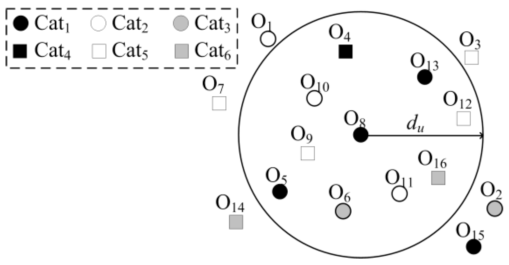
Recommendation systems can be used to obtain advice about any number of topics, such as locations and potential contacts [46].

Recommending Locations: Many recommendation systems generate lists of candidate POIs, regions, or sequential locations based on data obtained from LBSNs, such the profile, historical check-ins, and historical trajectories of the user. Initially, these systems were based on collaborative filtering [47,48], content-based systems [49], and knowledge-based systems [50]. For example, Abowd et al. [7] recommended POIs to users based on their locations and history. Considering the preferences, social networks, and locations of users, Ye et al. [8] used score functions to calculate the recommendation scores for POIs. Bao et al. [9] recommended POIs in accordance with check-in data. They first identified “experts” in the region of the user and then calculated recommendation scores based on the similarity of POI preferences between the experts and the user. Ying et al. [51] used check-in data to calculate similarity between the user and his/her social network, and then produced recommendations based on the preferences and popularity of POIs. Levandoski et al. [52] analyzed check-in history and geographical factors when recommending POIs. Liu et al. [53] developed the tourist-area-season topic model, which identifies potential travel packages based on topics and then generates personalized itineraries by combining POIs within defined limitations. Xie et al. [54] built independent recommendation systems based on type of POI, then employed the greedy algorithm concept to combine POIs by type into a portfolio, which was reviewed for compliance with the budget and time limitations of the user. Hsieh et al. [55] identified check-ins to must-go POIs and recommended the more popular destinations to users. Sang et al. [56] recommended multiple POIs based on the probability of traveling between POIs, which was calculated using check-in data, and the pathway probability, which was calculated using the Markov chain concept. Using previous check-in data, Lu et al. [57] calculated preference scores for POIs in unfamiliar cities, and checked to ensure that recommended itineraries were in line with the budget and time limitations of users.

Recent research on recommendation systems has focused largely on the use of conventional methods with multiple conditions, with a particular emphasis on time-related issues. Chiang et al. [58] claimed that the duration of a trip should be a key factor in any trip recommendation system. Based on the observation that users tend to visit different types of POI at different times, Lu et al. [57] suggested coordinating trip recommendations with trends extracted from the check-in records of attractions. Hosseini and Li [59] pointed out that temporal considerations could seriously affect the willingness of users to visit a given POI. Based on the observation that time-related factors are not necessarily applicable to every user or every dataset, Hosseini et al. [60] employed a probabilistic generative model to enhance the effectiveness of their recommendation system. Meng et al. [61] considered temporal considerations in calculating a time-sensitive QoS metric for their recommendation system. Cai et al. [62] treated temporal information as a key factor when seeking to compensate for sparse data. Ying et al. [63] merged context-aware tensor decomposition with time conditions in their recommendation system. Zheng et al. [64] sought to improve the accuracy and quality of recommendation systems by contrasting user sentiment with temporal conditions.

Other conditions can also be included in recommendation systems. Mukasa and Yamamoto [65] developed a recommendation system based on user priorities. Su et al. [66] and Huo et al. [67] considered issues pertaining to privacy in the formulation of recommendations. Gan and Gao [28] employed forgetting curves in their recommendation system. Li et al. [68] used semantic data to enhance the accuracy of location recommendations. Wang et al. [69] considered the degree of trust between users in their recommendation system. Mehmood [70] developed a recommendation system using the real-time data instead of the historical data. Logesh et al. [10] and Huang et al. [11] developed systems to recommend travel routes suitable for groups instead of individual users. Kang et al. [32] developed a recommendation system for online-to-offline commerce.

Another stream of research on location recommendation systems has focused on the adoption of more sophisticated methods, such as graph-based schemes and artificial intelligence. Guo [71] employed various graph-based methods to facilitate the generation of recommendations. Bin et al. [72] developed a route recommendation algorithm based on sequential patterns identified via data mining. Yang et al. [73] used a hidden Markov model to personalize potential routes. Using a deep neural network, Gao et al. [74] characterized POIs according to topic, identified user preferences, and extracted geographic details from LBSN records. Zhang et al. [75] developed a recommendation system based on the embedding of users and POIs in conjunction with a long short-term memory network to derive user preferences based on their check-in sequence, before using a fully-connected neural network to evaluate candidate recommendations. Liu et al. [76] developed the spatiotemporal dilated convolutional generative network for POI recommendation. Cao et al. [30] developed a recommendation system based on edge computing using LBSN data.

Despite the success of the above recommendation systems, their objectives and methods and were deemed unsuitable for the current study. Our objective was to identify suitable partners for a specific POI. We therefore did not consider the individual preferences or limitations of users. Rather, we focused on the link between POIs and the various attributes of their customers.

Recommending Potential Contacts: This type of recommendation system is used to generate recommendations pertaining to local experts/opinion leaders or potential friends based on data from LBSNs [46]. Many researchers have pointed out that location histories provide rich contextual information that is strongly correlated to social behaviors. Thus, it is reasonable to surmise that in characterizing relationships between users, data collected from LBSNs is more useful than information from non-LBSN platforms. Zheng et al. [12] developed the HITS inference model to search for travelers with experience in specific regions based on historical trajectories. Ying et al. [77] determined that users with a large number of trajectories are more likely to connect to other popular users, and is therefore a valuable resource in tracking down local experts or opinion leaders. Analysis of data collected from LBSN platforms led DeScioli et al. [13] to conclude that social connections are highly related to geographical distance. Zhu et al. [14] clustered users based on social trust in formulating recommendations of potential friends. Chen and Li [15] developed a novel graph embedding method to find potential propagators and customers in LBSNs. Pan et al. [78] used semantic information of users in LBSNs to generate recommendations of potential friends. Xin and Wu [79] used three user-related features extracted from LBSNs to train a modified support vector machine by which to predict links between users in order to generate friend recommendations.

3. Definitions

This section first defines some terms used in this work and then specifies our research goal.

Definition 1.

POIs. O = {o₁, o₂, ..., o_|O|} denotes the collection of POIs in a certain area.

We assumed that the model social network dataset included at least two types of data by which to characterize any POI mentioned in this paper, including discrete and continuous data. Discrete data included the POI rating, total check-in count, and prices/star rating, whereas continuous data included the age distribution of people visiting the POI. The definitions of these two types of data are as follows.

Definition 2.

Discrete attributes of POI. o_i.Ddata = {vd₁, vd₂, ..., vd_|Ddata|} indicates discrete field data obtained from social networks for POI o_i, which are expressed using single values.

Definition 3.

Continuous attributes of POI. o_i.Cdata = {vc₁, vc₂, ..., vc_|Cdata|} indicates continuous field data obtained from social networks for POI o_i, which are expressed using single vectors written as vc_j = {vc_j1, vc_j2, ..., vc_j|vc_j|}.

In addition, each POI o belongs to a category CAT(o). For each query, the user specifies a query POI q as the object of the query. The POIs can then be divided into competitors, and potential partners, which are defined as below.

Definition 4.

Competitor. CP(q, d_u) is the set of POIs which are in the same category as and within Euclidean distance d_u of POI q.

In the current work, Euclidean distance was used to evaluate the distance between two POIs. In the selection of joint promotion partners, the primary concern is whether a POI is located within or close to the business district of the user, and Euclidean distance is the most intuitive approach to describing proximal relationships of this type. Note also that our objective was to facilitate system implementation and obtain query results quickly (see Section 1). The low computational cost involved in calculating Euclidean distance was another benefit. Of course, if the system supplier were willing to install advanced servers, or if they wanted to alter the recommendation parameters, then they could evaluate distances using other methods, such as Mahalanobis distance, road distance, Manhattan distance, without fundamentally altering the system. Note that for the sake of simplicity, all distances mentioned hereafter refer to Euclidean distance.

By the way, the desired range for each query is dependent upon the POI owner, so the algorithm allows users to customize d_u.

Definition 5.

Potential partner. P(q, d_u) is the set of POIs which are in different categories from and within Euclidean distance d_u of q.

Definition 6.

Partner score. A partnership between potential partner o_i and q has a partner score PS(o_i,q) which denotes the suitability of the partnership. The higher PS(o_i,q) is, the more suitable the partnership between o_i and q is. This partner score is obtained by calculating the relationships among the discrete and continuous attributes of o_i and q.

After introducing the various definitions associated with POIs, we next define the topic of this study.

Official problem statement. The POI owner first provides values for a given set of parameters (q, d_u, k), where q is the location of the query POI, d_u is the user-provided distance limitation, and k is the number of candidates that the POI owner wishes to obtain. Based on these values, JPPRS returns a set of k POIs, which are potential joint promotion partners of q, where the distance from q to the furthest POI does not exceed d_u. In the event that the POI owner is unable to provide reasonable estimates for parameters d_u and k, then JPPRS can suggest suitable values in accordance with the city in which q is located.

Example 1.

In this section we use the example in Figure 1 to illustrate the definitions given above. Each object in this figure represents a POI and the objects with the same shape and color represent POIs from the same category. There are 16 POIs (i.e., O = {o₁, o₂, ...,o₁₆}), 6 categories (i.e., CAT = {cat₁, cat₂, ..., cat₆}), For example, o₅, o₈, o₁₃, o₁₅ are 4 POIs belong to cat₁. Suppose, the owner of o₈ requests a joint promotion partner within distance d_u and he sets k = 3. Object o₈ is then query POI q. With o₈ as the center, the distance range d_u from o₈ is marked in the figure by the line. {o₅,o₁₃} form the set CP(o₈, d_u), as they are in the same category as and within distance d_u of o₈. {o₄, o₆, o₉, o₁₀, o₁₁, o₁₂, o₁₆} is the set of potential partners P(o₈,d_u), because they are in different categories from and within distance d_u of o₈. The proposed system then returns results: {PS(o₄,o₈), PS(o₆,o₈), PS(o₉,o₈), PS(o₁₀,o₈), PS(o₁₁,o₈), PS(o₁₂,o₈), PS(o₁₆,o₈)} = {0.75, 0.23, 0.44, 0.31, 0.3, 0.7, 0.8}. o₁₆, o₄, o₁₂ are therefore suitable joint promotion partners for o₈, as they possess the top-3 highest scores from among all potential partners.

Ideal LBSN dataset format for JPPRS: Based on the definitions above, we suggest that the target LBSN include the five following tables: (1) POI location table listing the latitude and longitude of all POIs, (2) POI information table listing POI characteristics, such as prices and star ratings, (3) POI rating table listing the ratings assigned by the public and total check-in count, (4) User information table listing personal information of LBSN users, such as gender and age, and (5) User check-in table listing the POIs with the time of checks-ins and text comments. Note that the five tables listed above are made available by nearly all LBSNs. Using these five data tables, it should be possible to obtain all of the information required to make joint promotion partner recommendations, including the customer base, customer ratings, price/star ratings, and distance between the target POI and other POIs. The customer base can be derived from the user information table and user check-in table. We begin by collecting the Indexes and personal data of people that have visited the POIs of interest. We then obtain the customer rating of the POIs from the POI Rating Table as well as the prices/star ratings from the POI Information Table. Finally, the distances between POIs are derived from the POI Location Table using the Euclidean distance formula.

Note that in this paper, we consider only the five tables above in the implementation of JPPRS. This is because that our aim was to maximize the adaptability of JPPRS to different LBSNs and these five tables are almost all LBSNs dataset will have. Of course, system suppliers could make available additional tables to enhance the accuracy of their recommendation system.

4. Methodology

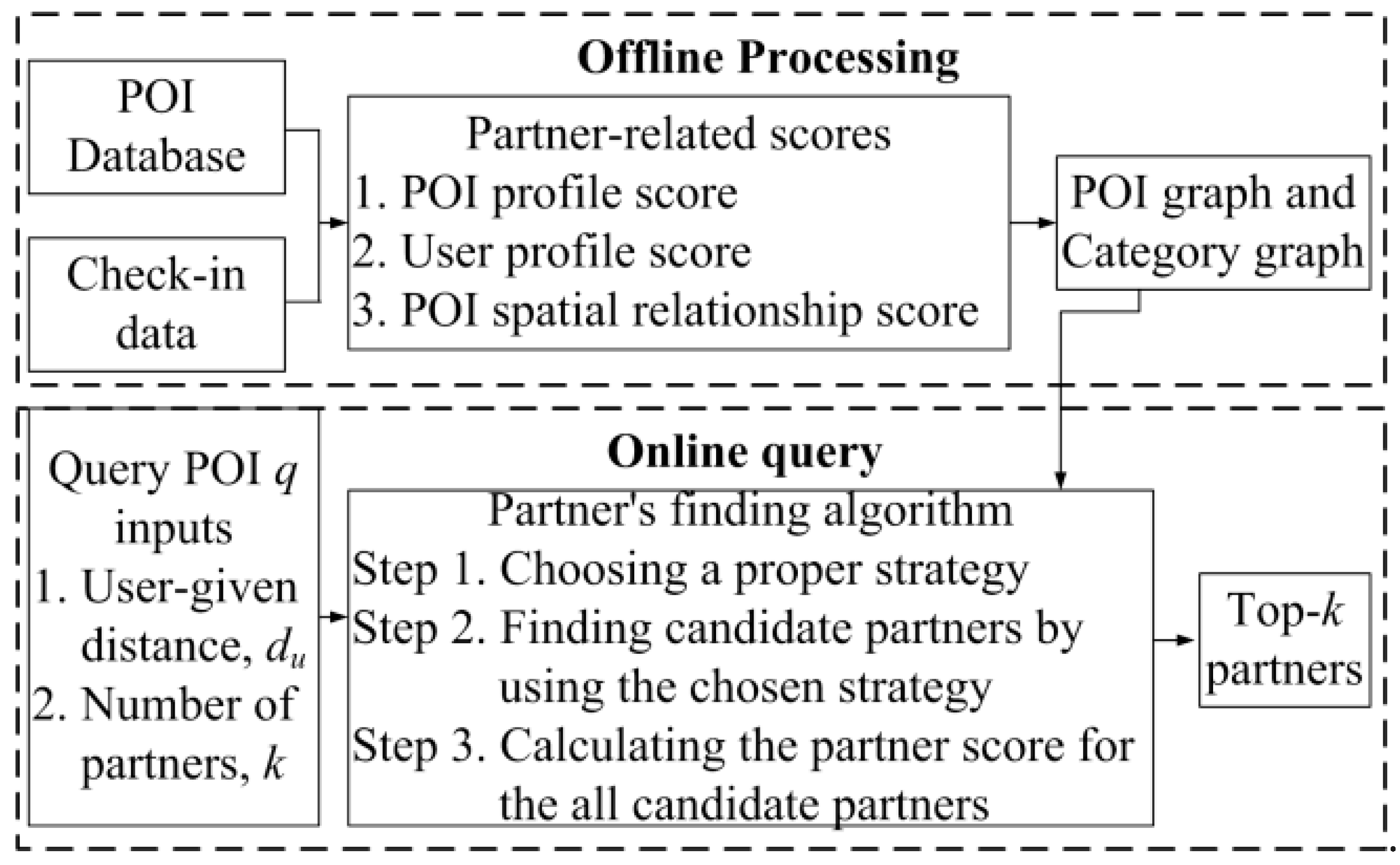
4.1. Framework of Joint Promotion Partner Recommendation Systems (JPPRS)

This paper presents a system that suggests an individualized set of joint promotion partners to the owners of a POI in real time. As illustrated in Figure 2, the JPPRS is implemented in two stages. The first stage is offline processing, which proceeds as follows. (1) Collecting data from the target LBSN. (2) The following three partner-related scores are then evaluated by considering the customer bases, customer ratings and awareness, prices and star ratings, and distance (i.e., the first five key factors mentioned in Section 1), including the POI profile score (PPS), the user profile score (UPS), and the POI spatial relationship score (SRS). (3) The three partner-related scores are then converted into a POI graph (PG) and category graph (CG) as the input data for the second stage.

The second stage is an online query, which considers the promotional strategies (i.e., the last key factor mentioned in Section 1) in its process. This stage requires distance d_u and the number of required partners k. Distance d_u is set by the user and represents the maximum acceptable distance between joint promotion partners. After receiving query POI q’s request, the Partners Finding algorithm uses three parts to find the top-k partners for q. The algorithm first selects a promotion strategy for q. It then finds candidate partners using the chosen strategy and the PG and CG. The last part of the algorithm uses a speed-up algorithm to calculate the partner score for all candidate partners, where partner score represents the suitability of collaboration between q and each candidate partner. The k candidate partners with the highest partner scores are selected as the top-k partners.

As mentioned previously, our objective was to facilitate system implementation and obtain query results quickly; therefore, we simplified the JPPRS algorithms as much as possible. Of course, if the system supplier were willing to install advanced servers, then more sophisticated algorithms could be adopted without difficulty.

4.2. Offline Processing

Offline processing involves calculation of three scores, PPS, UPS, and SRS, and construction of the PG and CG. To facilitate our explanation without the loss of generality, we assume that the model LBSN dataset used for analysis includes the five common tables, namely a POI location table, a POI information table, a POI rating table, a user information table, and a user check-in table. These five tables only include the simplest fields needed to explain the calculation details of various scores. For instance, the POI location table only contains the IDs, latitudes/ longitudes of the POIs; the POI information table only includes the prices and star ratings of the POIs; the POI rating table only contains the means of the scores given by all users; the user information table only presents the gender (discrete attribute) and age (continuous attribute) of the users, and the user check-in table only records the POIs that each user checked in at and their rating of the POI at the time. When users obtain other LBSN datasets in the future, they can customize the calculations to derive the PPS, UPS, and SRS corresponding to these LBSN datasets.

4.2.1. POI Profile Score (PPS)

The PPS is the measure of similarity between two POI profiles. The elements of a POI profile include (1) demographic data such as gender, and age, (2) customer response scores such as the rating of the POI and the total check-in count of the POI, and (3) other information related to the POI such as prices and star ratings. Analysis of this score reveals information relevant to three factors of partner selection: (1) the extent to which the POIs share a market; (2) similarity between two POIs in terms of rating and awareness and (3) similarity in terms of prices and star ratings. POI profiles include discrete data, such as the gender of customers, appraisal of POI, total check-in count, prices, and star ratings, and continuous data, such as customer age. Different methods are used to process discrete and continuous data; therefore, we processed each type of data separately and then computed the mean score as described below.

Similarity Among Discrete Data: Discrete data in a POI profile includes the gender of customers, their appraisal of the POI, the total check-in count, prices and star ratings. Customer c is defined as an individual who has previously checked in to POI o.

Table 1. Calculation of similarity among discrete data.

Attributes\POIs		o1	o2	o3
Gender	Male	0.3	0.8	0.4
	Female	0.7	0.2	0.6
Rating		4(0.8)	3.5(0.7)	4.2(0.84)
Total check-in count (unique customers)		5000(0.25)	150(0.0075)	4000(0.2)
Price		5(0.01)	500(1)	3.5(0.007)
Star rating		0(0)	5(1)	0(0)

presents an example of a POI profile in terms of discrete attributes, which were all obtained from our model LBSN dataset. First, Gender represents the gender statistics of the customers that had visited POIs o₁, o₂, and o₃. To calculate these fields, we first found the indexes of the customers that had been to o₁, o₂, and o₃ and then obtained the genders from these indexes. In this field, the gender values for o₁ are 0.3 for male and 0.7 for female, meaning that 30% of the customers going to o₁ are male and 70% are female. Next, the ratings, total check-in counts, prices, and star ratings of POIs o₁, o₂, and o₃ are directly obtained from POI information table and the POI rating table in the model LBSN dataset, with no calculations needed. As these four parameters cannot be proportionally compared, we compared them using the normalization [0, 1] method. The numbers not enclosed in parentheses are the actual figures, whereas the figures in parentheses are normalized using the maximum data set. Assuming that the rating range is zero to five, and the rating of o₁ is four, then the normalized rating of o₁ would be 0.8. that the maximum value is 20,000; therefore, the normalized score is 0.25. Price refers to the average prices of services and products offered by the POI. We set the maximum price at USD500. Rating, which symbolizes the quality of the POI, has a range of zero to five stars, with higher star ratings indicating higher-end products and services. Assuming that the discrete data vector of POI o_i has m dimensions, then the vector can be expressed as [PP_dis,i,1, PP_dis,i,2, PP_dis,i,3…PP_dis,i,m], where PP indicates the POI profile. In Table 1, for example, the discrete data vector of o₁ is [0.3, 0.7, 0.05, ..., 0.25, 0.01, 0]. We can calculate the similarity among discrete data between POI o_i and o_j using the cosine similarity [52,57] as follows:

$$P{P}_{dis}Sim\left(o_i,o_j\right)=\frac{{\displaystyle {\sum }_{n=1}^m\left(P{P}_{dis,i,n}\times P{P}_{dis,j,n}\right)}}{\sqrt{{\displaystyle {\sum }_{n=1}^{m}P{P}_{dis,i,n}{}^2}}\times \sqrt{{\displaystyle {\sum }_{n=1}^{m}P{P}_{dis,j,n}{}^2}}}.$$

(1)

Similarity Among Continuous Data: In calculating the PPS, we often encounter continuous data. Below, we use the age distributions of the customers who have been to a POI as an example to explain how to calculate the PPS scores of continuous data obtained from the user information table of the model LBSN dataset. We first found the indexes of the customers that had been to o₁, o₂, and o₃ and then used those indexes to calculate how many customers of each age had been to these POIs, as shown in Figure 3. At age 20 on the x axis, the values for o₁, o₂, and o₃ are 330, 0, and 300, respectively. This indicates that 330, 0, and 300 customers aged 20 had visited o₁, o₂, and o₃. We use these two curves to calculate the similarity among the continuous data of two POIs. We also incorporated the Pearson correlation coefficient [80]. The results range from -1 to 1, where 1 indicates that both curves are fully consistent (identical), 0 indicates a high level of inconsistency (dissimilar), and -1 indicates that the curves are completely opposed (no similarity whatsoever). Equation (2) presents the Pearson correlation coefficient.

$$P{P}_{dis}R\left(o_i,o_j\right)=\frac{Cov\left(P{P}_{cont,i},P{P}_{cont,j}\right)}{\sigma \left(P{P}_{cont,i}\right)\times \sigma \left(P{P}_{cont,j}\right)},$$

(2)

where Cov(•) is the statistical covariance and σ(•) is the standard deviation of the curve. Note that the covariance can be further evaluated by the following equation

$$Cov\left(P{P}_{cont,i},P{P}_{cont,j}\right)=\frac{{\displaystyle \sum _{n=\alpha }^{\beta }\left[\left(P{P}_{cont,i,n}-\mu \left(P{P}_{cont,i}\right)\right)\times \left(P{P}_{cont,j,n}-\mu \left(P{P}_{cont,j}\right)\right)\right]}}{\left(\beta -\alpha \right)},$$

(3)

where σ(PP_{cont, i}) is the standard deviation of the continuous data set of o_i, as shown in Equation (4):

$$\sigma \left(P{P}_{cont,i}\right)=\sqrt{{\displaystyle \sum _{n=\alpha }^{\beta }\left[{\left(P{P}_{cont,i,n}-\mu \left(P{P}_{cont,i}\right)\right)}^2\right]}/\left(\beta -\alpha \right)},$$

(4)

where μ(PP_{cont, i}) represents the mean of the continuous data set of POI o_i, as shown in Equation (5):

$$\mu \left(P{P}_{cont,i}\right)={\displaystyle \sum _{n=\alpha }^{\beta }P{P}_{cont,i,n}}/\left(\beta -\alpha \right).$$

(5)

Referring to Figure 3 as an example, the similarity between the age curves of o₁ and o₂ is R_age(o₁, o₂) ≈ 0.142 and R_age(o₁, o₃) ≈ 0.907. Finally, we can get PP_contSim(o_i, o_j) by using Equation (6):

$$P{P}_{cont}Sim\left(o_i,o_j\right)=R_{age}\left(o_i,o_j\right).$$

(6)

After calculating the similarity among the discrete and continuous data of POIs o_i and o_j, we can obtain their POI profile score PPS(o_i, o_j) as shown in Equation (7):

$$PPS\left(o_i,o_j\right)=\left({\mathrm{PP}}_{dis}Sim\left(o_i,o_j\right){+\mathrm{PP}}_{cont}Sim\left(o_i,o_j\right)\right)/2.$$

(7)

4.2.2. User Profile Score (UPS)

UPS is mainly used to express the preferences of all customers for two POIs, o_i and o_j. This can be calculated using the POI rating fields in the user check-in table of the LBSN.

Table 2. Customer preferences in relation to o_i and o_j.

c v.s. oj\c v.s. oi	Don’t Like oi, [0, 0.33)	Don’t Rule Out oi, [0.33, 0.67)	Like oi, [0.67, 1]
Like oj [0.67, 1]	(1) ≈0%	(2) ≈75%	(3) ≈100%
Don’t rule out oj, [0.33, 0.67)	(4) ≈0%	(5) ≈50%	(6) ≈75%
Don’t like oj, [0, 0.33)	(7) ≈0%	(8) ≈0%	(9) ≈0%

illustrates how these preferences are quantified, where c indicates any one of the customers. The columns indicate how much c likes o_i, while rows indicate how much c likes o_j. Finally, the percentage figure beside each scenario represents the probability that c would participate in a joint promotion combining o_i and o_j. Note that although the preferences in this table are divided into three ranges: [0,0.33], [0.33,0.67], and [0.67,1], in a real-life scenario, the preferences of c with regard to POI can be divided into smaller ranges. The probability in this table will be decided case by case.

Based on the value intervals in the Table 2, we can distinguish nine different reactions of c to o_i and o_j. For example, scenario (7) is that c doesn’t like o_i or o_j. In scenario (4), c doesn’t like o_i but does not rule out o_j. Scenario (1) is that c does not like o_i but does like o_j. Next, for each scenario, users can assign a reasonable probability for them. For example, in scenario (7) c doesn’t like o_i or o_j; therefore, the probability of c participating in the aforementioned campaign would be 0%. In contrast, c likes both o_i and o_j in scenario (3), indicating 100% probability that he would participate in the promotional activity. These scenarios show that the greater the preference of c for o_i and o_j, the more likely he is to participate in the joint promotion.

There are many scenarios, such as (1), (4), (8), and (9), in which c likes only one or the other of the POIs. In these circumstances, the probability of c participating in the joint promotion approaches 0. This is because even though c is willing to visit one POI, he or she is unlikely to join the joint promotion because of dislike for the other POI. In scenarios (2) and (6), it is still quite probable that c will participate in the joint promotion, because he or she does not harbor any particular dislike of either POI. In this situation, a promotional discount or special offer may attract him to participate. This shows that c is more likely to participate in the joint promotion if he does not have significantly different feelings about o_i and o_j.

The above analysis shows that UPS is associated with: (1) maximum preference for o_i and o_j, and (2) minimal difference in preference for o_i compared to o_j. These two factors increase the probability that customer c will participate in a joint promotion combining o_i and o_j. The more customers meet these criteria, the more participants the joint promotion will have, which increases its chances of success. Hence, we define UPS as follows:

$$UPS\left(o_i,o_j\right)={\displaystyle \sum _{\forall c\in c\left(o_i\right)}\left[\left(pref\left(c,o_i\right)+pref\left(c,o_j\right)\right)\times \left(1-\left|pref\left(c,o_i\right)-pref\left(c,o_j\right)\right|\right)\right]/\left|c\left(o_i\right)\right|},$$

(8)

where o_i, o_j are any two POIs; c(o_i) is the customer set of o_i; |c(o_i)| is the total number of customers for o_i; and pref(c, o_i) is the preference of c for o_i. Therefore, pref(c, o_i)+ pref(c, o_j) is used to calculate the total of preference for o_i and o_j, and 1-|pref(c, o_i)-pref(c, o_j)| calculates the difference in preference for o_i compared to o_j.

We now discuss calculation of pref(c, o_i), which is the measure of how much customer c likes POI o_i. Social networks offer many methods for computing the degree of user preference for a POI. We selected the check-in frequency method [9,57], which is the most commonly used approach and involves calculating the frequency with which c checks into POI as a percentage of his or her total check-in count (see Equation (9)).

$$pref\left(c,o_i\right)=c.o_{i}t/c.tct,$$

(9)

where c.tct represents the total check-in count of c, and c.o_it represents the frequency with which c checks in to o_i. The higher the score of c.o_it as a proportion of c.tct, the more the customer is seen to like POI o_i. Using

Table 3. Example of calculation of degree of preference and UPS.

	o1	o2	o3	...	Total
c1	10	0	1	…	20
c5	30	3	10	…	60
c14	25	5	25	…	60
c19	12	0	0	…	15

as an example, the preference of c₅ for o₁ is 30/60 = 0.5 and the preference of c₁₄ for o₁ is 25/60 = 0.41667. Using Equation (9), we can update Equations (8) to (10).

$$UPS\left(o_i,o_j\right)={\displaystyle \sum _{\forall c\in c\left(o_i\right)}\left[\frac{c.o_{i}t+c.o_{j}t}{c.tct}\times \left(1-\frac{\left|c.o_{i}t-c.o_{j}t\right|}{c.o_{i}t+c.o_{j}t}\right)\right]/\left|c\left(o_i\right)\right|}.$$

(10)

We discuss below how to use Equation (10) to calculate UPS(o_i, o_j) employing Table 3 as an example. Assuming that o₁ has only four customers c₁, c₅, c₁₄, c₁₉, then UPS(o₁,o₂) = (0 + 0.1 + 0.167 + 0)/4 ≈ 0.07, UPS(o₁, o₃) = (0.1 + 0.333 + 0.833 + 0)/4 ≈ 0.317. Note that in our study, because the two POIs may have different customer groups (i.e., C(o_i) may ≠C(o_j)), UPS(o_i, o_j) may ≠ UPS(o_j, o_i).

4.2.3. POI Spatial Relationship Score (SRS)

The SRS is calculated as the distance between the two POIs. This score is relevant because the distance between two POIs impacts on customers’ willingness to travel from one to the other [81]. This score can be obtained by applying the Euclidean distance formula to the latitudes and longitudes of the POIs in the POI location table of the LBSN. Generally speaking, customers are more willing to visit two POIs that are located within a reasonable distance from each other. If the distance between them is too great, customers will be less motivated to make the effort. Once the distance exceeds a certain parameter, customers are highly unlikely to travel between the POIs, making partnership unfeasible. We therefore incorporated a distance threshold and distance factor to calculate how distance affects the possibility of partnership between two POIs. If the distance exceeds the threshold d_t, then the two POIs cannot partner. If the distance is less than d_t, then the distance factor comes into play. Transport systems and commuter habits differ from city to city, so we cannot apply the same d_t and distance factor uniformly. We therefore analyzed check-in data related to different cities to determine their d_t and distance factors. This process is illustrated below.

First, we convert historical check-in data to continuous check-in data.

Table 4. An example of check-in data.

Customer ID	Time	Location
0005	2015/05/06/09:00	o1
0421	2015/05/06/14:15	o3
0005	2015/05/06/15:30	o2
0005	2015/05/06/19:00	o15
…	…	…
0158	2015/06/11 19:00	o9

shows the check-ins of a single customer on a given day. Customer ID 0005 checked in at three locations, o₁, o₂, and o₁₅, on 6 May 2015. Next, we can link any two continuous POIs into a pathway. For example, o₁ and o₂ form a single pathway, and o₂ to o₁₅ form a separate pathway. The great circle distance equation [82] is then used to calculate the distance of each pathway. Lastly, we count the distances of all pathways, leading to results such as those illustrated in Figure 4. The dotted line shows the percentage of pathways in each respective distance interval, while the solid line shows cumulative percentages. According to the concept of normal distribution, we set d_t as a cumulative percentage of 95%. Pathways are unlikely to fall outside of these parameters.

After calculating distance threshold d_t, we computed the spatial relationship score SRS(o_i, o_j) of two POIs, o_i and o_j, as shown in Equation (11).

$$SRS=\{\begin{array}{c}\left(1-dist\left(o_i,o_j\right)/d_t\right),dist\left(o_i,o_j\right)\le d_t\hfill \\ 0 ,dist\left(o_i,o_j\right)>d_t\hfill \end{array},$$

(11)

where dis (o_i, o_j)/d_t is divided by d_t in order to normalize the distance to a value between 0 and 1. The smaller the value of dis (o_i, o_j)/d_t the better; therefore, the greater the result of 1- dis (o_i, o_j)/d_t the better.

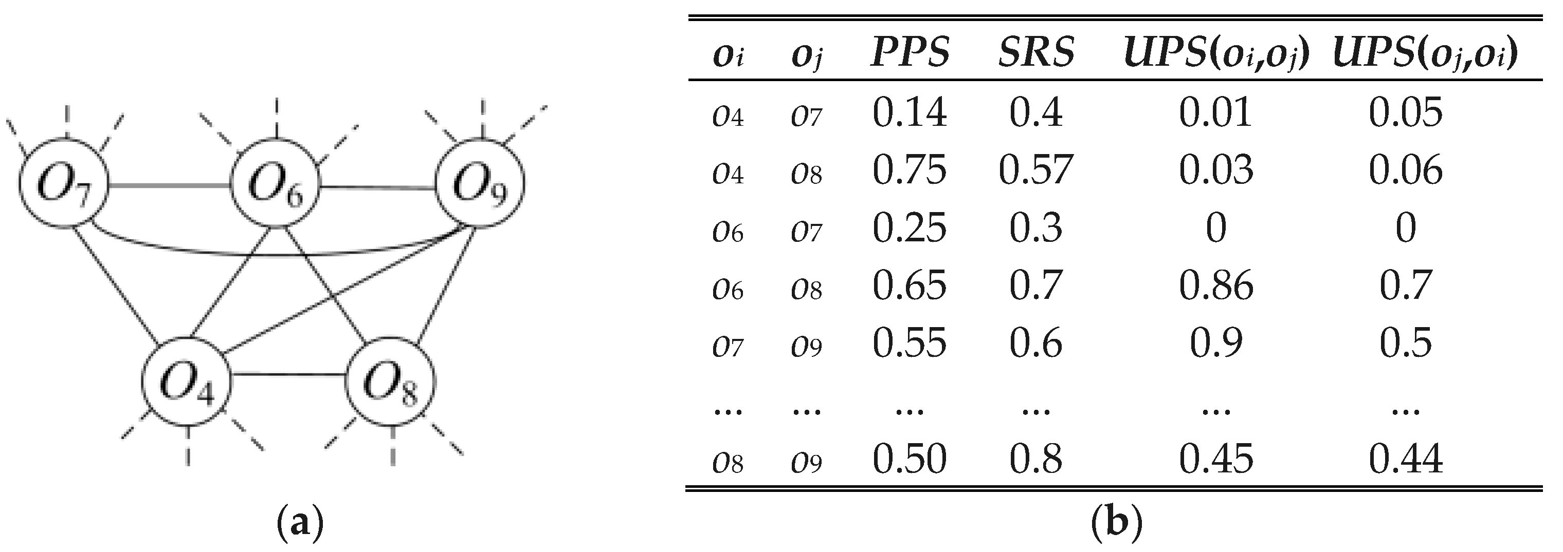
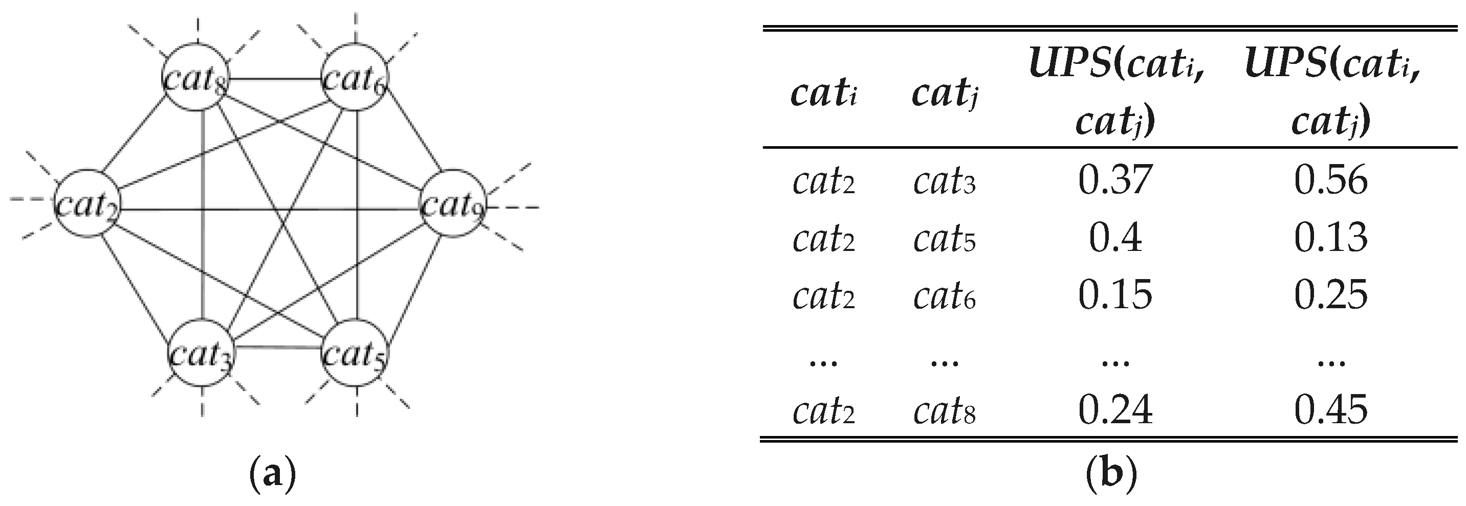
4.2.4. POI Graph and Category Graph

POI and category graphs are built to enable search functions in response to online queries. The POI graph records the POI profile, user profile and spatial relationship scores of any two POIs, and can aid the algorithm in finding potential partners for query q. However, we found that although the three types of scores stored in this graph are helpful in calculating the preferences of customers who have been to q, they do not consider customers who have not yet visited q. We therefore used the category graph to calculate the preferences of customers who have never been to q. This graph records the relationships between POIs in different categories; for example, the relationship between a POI selling bread and a POI that is a cafe. In this situation, as long as we know which category query POI q belongs to, we can access data on customers who have not previously visited q. In the sections below, we detail the development of these two types of graphs.

POI Graph: This undirected graph is formed from the POI O set and the three scores UPS, PPS, and SRS. Figure 5 is an example of a POI graph, where all POIs are connected by edges except for those belonging to the same category. Each edge shows the PPS, UPS, and SRS scores of two POIs, forming [PPS, SRS, UPS(o_i,o_j), UPS(o_j,o_i)], where i is less than j. Note that there are two UPS scores on the edge, because UPS(o_i,o_j) and UPS(o_j,o_i) are usually different and have to be recorded separately. In Figure 5, for instance, assume that o₈ and o₇ belong to the same category, so they are not connected. The scores [0.5, 0.8, 0.45, 0.44] for o₈ and o₉ represent PPS(o₈,o₉) = 0.5, SRS(o₈,o₉) = 0.8, UPS(o₈,o₉) = 0.45, and UPS(o₉, o₈) = 0.44. Notably, Figure 5 shows scenarios in which the UPS of two POIs equal 0; for example, UPS(o₆, o₇) and UPS(o₇, o₆) both equal 0. This is because o₆ and o₇ share no customers.

Category Graph: The structure of a category graph is similar to that of a POI graph, as shown in Figure 6. Nodes are shown as categories, while edges represent the correlation scores between categories.

The difference between the two graphs is that in a POI graph, the edges record PPS, UPS and SRS, while the category graph shows only UPS. The reason that PPS is not calculated is because despite belonging to the same category, two POIs can attract customers with significantly different attributes. For example, some cafes may be designed to appeal to an older crowd, while others target young customers. In this case, calculating PPS would be completely meaningless. We are unable to calculate SRS between two categories because each category contains multiple POIs, and we cannot calculate the distance relationships among multiple POIs.

In a category graph, UPS can be calculated using Equation (12). Assuming that category cat_i includes POIs o_i,1, o_i,2, ..., o_i,m, and category cat_j comprises POIs o_j,1, o_j,2, ..., o_j,n, we can calculate the user profile score UPS(cat_i, cat_j) as follows:

$$UPS\left(ca{t}_i,ca{t}_j\right)={\displaystyle {\sum }_{k=1}^m{\displaystyle {\sum }_{l=1}^{n}UPS\left(o_{i,k},o_{j,l}\right)}}/\left|m\times n\right|,$$

(12)

where UPS(o_i,o_j) is calculated using Equation (10).

4.3. Online Query

The online query stage of JPPRS has three processes: (1) selection of the most appropriate promotion strategy for query POI q, (2) finding candidate partners using the chosen strategy, and (3) calculation of the partner score for the candidate partners using the speed-up algorithm.

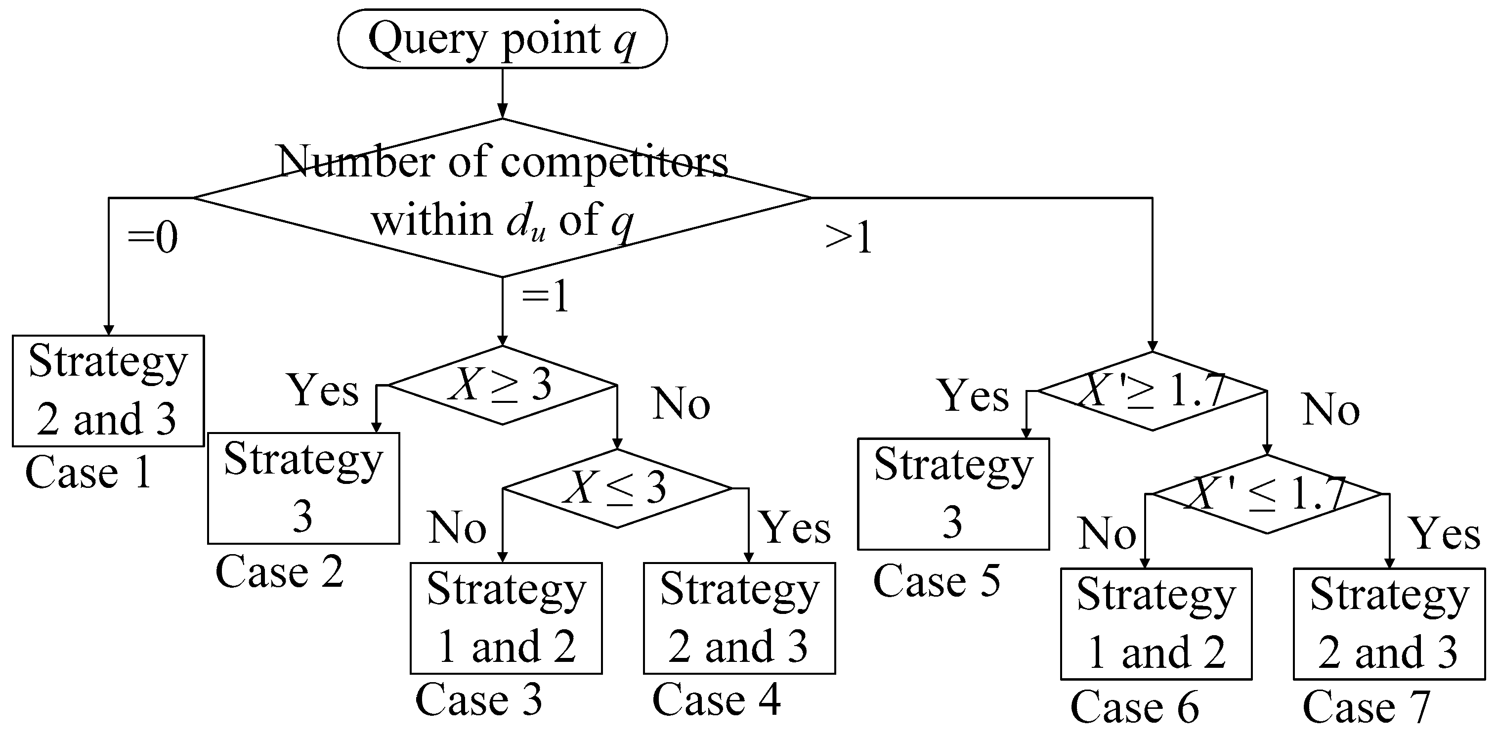
4.3.1. Promotion Strategy Selection

Joint promotion is a frequently discussed topic that has many commercial applications [1,83]. One of the most well-known joint promotion theories is Lanchester’s law [84,85,86], which is a wide-ranging concept that covers mathematical analysis, modeling, and theoretical deduction. This study used only the shooting range theory [87] of Lanchester’s law to select an appropriate strategy for query POI q. By strategy we mean the methods of setting and achieving targets, and allocating required information. In the sections below, we explain how to use the shooting range theory of Lanchester’s law to formulate strategies. This theory includes the following two theorems.

Theorem 1.

Only two businesses of the same type within the same area are referred to as A and B. If the market share of A is three times or more that of B, then B cannot compete for the customers of A. Conversely, A and B would be able to compete for each other’s clientele.

Theorem 2.

If there are three or more businesses of the same type in the same area, as long as the market share of A is at least 1.7 times that of any of the others, the so-called B, then B cannot compete for A’s customers. If not, however, then A and B can compete for each other’s customers.

Based on Theorem 1 and 2, we categorized market competition between the POIs into seven potential scenarios, corresponding to three different strategies. There are one to two response strategies to each scenario (Figure 7). Our three response strategies are discussed below, followed by the seven market scenarios. We designated the query POI as q, and assumed that POIs of the same category as q are its competitors. Competitors that have comparable market share to q and therefore pose a reasonable threat are referred to as real competitors. We used user-given distance d_u to define the ’area’ referred to in Theorems 1 and 2.

Our three response strategies are as follows:

Strategy 1. Attracting customers from real competitors: The objective of this strategy is to attract the customers of real competitors. To achieve this objective through a joint promotion, q must identify POIs that share the same customer groups as the real competitors, and then partner with those POIs to employ new promotional activities to attract customers.

Strategy 2. Protecting one’s own customer base: The objective of this strategy is to prevent the loss of existing customers. To achieve this goal through a joint promotion, q must identify what other POIs its customers like to frequent, and partner with those POIs in a joint promotion. This provides the customers of q with a strong incentive to keep coming back to q to consume.

Strategy 3. Attracting potential customers: This strategy aims to attract potential new customers. We must first identify POIs with clientele who may be interested in q, and then partner with POIs from that category to host a joint promotion. The reason that we first evaluate POIs by category is because there may be many POIs in one city, and assessing their customer groups individually would be too time-consuming. Our approach reduces the number of POIs to be processed and therefore accelerates computational speed.

Next, we outline the seven market scenarios of Figure 7. Note that for the ease of explanation, the value of (market share of q/market share of competitor) is defined as X in the following.

In Case 1, d_u has no competitors at all. Without an opportunity to attract the customers of competitors (i.e., Strategy 1), the only remaining options are to protect its own customer base or attract potential customers (i.e., Strategies 2 and 3).

In Cases 2 to 4, there is only one competitor within d_u of q:

In Case 2, there is only one competitor within d_u and X ≥ 3. In this situation, other POIs will not be able to attract the customers of q (Theorem 1) and will even lose money in the process of attempting to. Therefore, q does not need to worry about protecting its existing customers (i.e., Strategy 1) and can focus on the other two strategies. However, because the market share of competitors is significantly lower than that of q, there is no need to attract customers from competitors. Therefore, q need only focus on attracting potential customers (i.e., Strategy 3).

In Case 3, there is only one competitor within d_u and X is within the range of [1/3, 3], meaning that q and its real competitor both have a chance of attracting each other’s customers (Theorem 1). Therefore, q must focus on luring the customers of its real competitor (i.e., Strategy 1) as well as consolidating its existing customer base (i.e., Strategy 2), in order to gain greater market share. In this scenario, it is not necessary to attract new customer groups (i.e., Strategy 3).

In Case 4, there is only one competitor within d_u and X ≤ 1/3. This means that q cannot compete for the customers of its competitor (Theorem 1) and can only employ Strategies 2 and 3 to protect its existing customer base while attracting potential new customers. In Cases 5 to 7, multiple competitors are within d_u of q. We discuss different cases and response strategies below, where the value of (market share ratio between q and these competitors) is defined as X’.

In Case 5, there are two or more competitors within d_u, and X’ ≥ 1.7. In this scenario, no competitors can compete for q’s customers (Theorem 2), and it would not be efficient for q to attempt to attract the customers of its competitors. Therefore, q need focus on developing new customer groups (i.e., Strategy 3).

In Case 6, there are two or more competitors within d_u, and X’ is within the range of [10/17, 1.7]. This means that q and its competitors all have the opportunity to attract each other’s customers (Theorem 2). For this reason, q should employ Strategies 1 and 2 to attract the customers of its real competitors while protecting its own customer base.

In Case 7, there are two or more competitors within d_u, and X ’≤ 10/17. This means that q cannot attract customers from its competitors (Theorem 2) and must protect its own customer base as well as generate new business (i.e., Strategies 2 & 3).

Note that in some unusual cases, the predetermined strategies may fail to identify k number of partners; in such cases, we apply additional strategies. For example, if the results of Strategies 1 and 2 in Case 6 did not meet the requirement for k partners, we would then apply Strategy 3 to make up the difference.

The above discussion shows that market share is an important factor in the evaluation of the competitiveness of a POI. Equation (13) shows how we calculate market share using check-in data:

$$MS\left(o_i,O_{MS}\right)=\left(o_i.tct/{\displaystyle {\sum }_{\forall o\in O_{MS}}o.tct}\right)\times 100\%,$$

(13)

where o_i is the POI for which we are calculating market share; O_MS is the set of POIs in the same category as query POI q, and o.tct is the total check-in times of a POI (o∈O_MS). Higher check-in times implies greater market share.

Figure 1 presents an example of the process of strategy selection on the basis of check-in data, where o₈ = query POI q. Within the given range shown in the figure, o₈ has two competitors: o₅, and o₁₃. Given the check-in frequencies of o₅, o₈ and o₁₃ as 100, 150, and 180 times, respectively, then market share is calculated as follows: 100/(100+150 +180)*100%=23%; 150/(100+150+180)*100% = 35%, and 180/(100+150+180)*100% = 42%. In this example, o₈ has multiple competitors and its market share ratio to at least one of these competitors is within the range of [10/17, 1.7]. This is considered a Case 6 scenario. This means that o₈ should employ Strategies 1 & 2. If it is still unable to identify k partners, then we will apply Strategy 3 to source enough partners to meet the requirement.

4.3.2. Finding Candidate Partners

After selection of appropriate strategies for query POI q, the next step is to employ these strategies to select candidate partners. In this section we explain how to use POI graphs (PG) and category graphs (CG) to find candidate partners for the three abovementioned response strategies.

Strategy 1. Attracting customers from real competitors: In this strategy, q must identify the POIs that share customers with its real competitors. These POIs are the nodes linked to q and its real competitors in the PG. The UPSs for q, real competitors, and these nodes must also exceed a certain threshold. We need only identify these nodes in order to find candidate partners for q. Note that the PG enables us to easily calculate the three scores for any two POIs. The UPS threshold must be considered in order to eliminate those POIs that do not share customers with q or whose customers are unlikely to participate in promotional activities. For example, if the UPS threshold of Figure 5 is set at 0.1, o₈ is the query POI q, and o₇ is the real competitor of o₈. The selected node is o₉ because it is linked to both o₇ and o₈, and the UPS score exceeds 0.1, indicating that many customers of o₉ visit o₈ and o₇. For these reasons, o₉ is a candidate partner of o₈. Although o₄ is linked to o₇ and o₈, it was not selected because the UPS results were 0.01 and 0.03, i.e., less than 0.1. The probability that the customers of o₄ will participate in the promotional activity is therefore too low. Likewise, o₆ was not selected because its UPS in relation to o₇ equaled 0, indicating that it shares no customers with o₇.

Strategy 2. Protecting one’s own customer base: To implement this strategy q must identify POIs frequented by its existing customers and partner with these POIs in joint promotion. Customers are then encouraged to continue to frequent this POI in order to participate in the promotion. To identify suitable partners, we must identify nodes that are linked to q and have UPS above a predefined threshold. As for Strategy 2, threshold values are considered to eliminate those POIs that do not share customers with q or whose customers are unlikely to participate in promotional activities. For example, if the UPS threshold of Figure 5 is set at 0.1 and the candidate partners are o₆ and o₉.

Strategy 3. Attracting potential customers: The aim of this strategy is to attract potential customers (those who have not previously been to q but are likely to be interested in doing so). Because these individuals have never visited q, we are unable to obtain data using the PG, as the PG only records data on customers who have been to q at some point. We instead use the category graph (CG) to identify the category cat_q. of q. We next identify which additional categories the customers of cat_q also enjoy (using UPS value). The POIs in such categories are the candidate partners of q. Figure 6 shows an example in which query POI q belongs to cat₈, and cat₈ customers also like cat₂, cat₃, cat₅ and cat₆. Therefore, the POIs in these categories are all candidate partners.

4.3.3. Partner Score Calculation

After identifying all candidates, we calculate the fit between each candidate partner p_cand and query POI q. The calculation is a two-part process. We first calculate the willingness of q to collaborate with any p_cand,, (W(q, p_cand)) and vice versa (W(p_cand, q)). Note that W(q, p_cand) and W(p_cand, q) may not be the same, because q may want to partner with a certain p_cand, but that p_cand may not be willing to collaborate with q. We next use W(q, p_cand) and W(p_cand, q) to calculate the feasibility of partner score between q and any p_cand PS(p_cand, q). We can calculate the willingness score of a POI o_i to collaborate with another POI o_j as follows:

$$W\left(o_i,o_j\right)=[\alpha \times PPS\left(o_i,o_j\right)+\beta \times UPS\left(o_j,o_i\right)+\left(1-\alpha -\beta \right)\times SRS\left(o_i,o_j\right)],$$

(14)

where α and β are user-given parameters. The three scores are obtained from PG and CG and do not need to be separately calculated, which reduces computational time.

The partner score PS(o_i, q) is then calculated from the above results, as shown in Equation (15):

$$PS\left(o_i,q\right)=[W\left(o_i,q\right)+W\left(q,o_i\right)-\frac{\left|W\left(o_i,q\right)-W\left(q,o_i\right)\right|}{W\left(o_i,q\right)+W\left(q,o_i\right)}].$$

(15)

Note that W(o_i, q)+ W(q, o_i) is the sum total of partnership feasibility between the two POIs. Generally speaking, the higher this score, the higher the partner score. However, there are exceptions to this guideline. If the values of W(o_i, q), W(q, o_i) vary too greatly, this may be reduce their partnership feasibility, even if the sum total is high. We therefore subtract |W(o_i, q) − W(q, o_i)|/(W(o_i, q) + W(q, o_i)) to avoid this situation. Note that the difference between the POI scores is divided by W(o_i, q) + W(q, o_i) for normalization.

4.3.4. Partners Finding Speed Up Algorithm

Note that the most intuitive way to find the top-k partners for a query POI q is to calculate the partner score for each candidate partner node and q and retrieve the first k candidate partners with the highest scores. However, this method can be quite inefficient. Hence, we developed the Partners Finding Speed Up Algorithm to solve this problem. This algorithm reduces the computational load using the regressive SRS scores between candidate partners and q in Equation (14). The candidate partners are first arranged from smallest to largest according to their distance from query POI q. The k candidates closest to q are considered to be the top-k partners. Each of the other candidates is then examined to see if it can replace any of the top-k partners, starting with the (k + 1) candidate closest to q. This is determined as follows: Assuming that the minimum partner score of top-k partner is S_lowest, then the candidate to be examined is p_cand. The first step is to calculate the maximum score of p_cand (i.e., S_pcand,_highest) with a given SRS:

$$s_{p_{cand},highest}=2\left[\left(\alpha +\beta \right)+(1-\alpha -\beta )SRS\right],$$

(16)

To develop Equation (16), we replaced PPS and UPS in Equation (14) with 1 and then integrated it with Equation (15). If the score is lower than S_lowest, then all the candidates after p_cand cannot be top-k partners, so the evaluation is complete. Conversely, however, if the score exceeds S_lowest, then all the candidates after p_cand have a possibility of being top-k partners. We continue this process until all candidates have been examined and the remaining top-k partners are the final partners of q.

5. Experiments

In this section, we examine (1) the data and setup used in the experiments; (2) The conditions of various response strategies; (3) A performance comparison with one baseline algorithm and various relevant algorithms, (4) A case study to verify the applicability of the proposed algorithm, and (5) Experiment results. All experiments were implemented in Java running on Windows 7 64-bit using an Intel Core i7-870 4-core CPU with clock speed of 3.2 GHz and 8 GB of RAM. We opted for JAVA rather than other programming languages because JPPRS is meant to perform back-end calculations and present the results via a webpage. JAVA is one of the most common languages used for back-end algorithms.

5.1. Experiment Settings

We first introduce the data used in the experiment, which comprised the New York City dataset in the Foursquare dataset [52,88]. Note that we used the Foursquare dataset rather than other LBSN datasets to search for joint promotion partners for the three following reasons. (1) The Foursquare platform is an LBSN; therefore, its dataset contains a substantial amount of location-related information, which facilitates the investigation of spatial relationships between POIs. (2) The Foursquare dataset is one of the few LBSN datasets that are accessible, and this has made it a benchmark dataset for LBSN-related research. (3) Careful management of the Foursquare dataset ensures that the data fields and details are complete, while avoiding the issues imposed by having to use APIs or web crawlers to capture datasets from other LBSNs. Note that there are various versions of the Foursquare dataset, each of which differs slightly in terms of locations, information fields, and number of items. We opted for the Foursquare dataset version suggested in [52,88], due to the fact that the included data and fields were the best fit for this study. The details of the Foursquare dataset we used are shown in

Table 5. Foursquare dataset.

Description	Dataset	Description	Dataset
Number of POI check-ins	155,637	Time period	2011/12/08–2012/04/23
Number of paths	12,574	Number of categories	425
Number of users	81,685	Distance threshold dt	20.24
Number of users’ rating	166,585	Number of POIs	7691

. This dataset includes 155,637 pieces of check-in data, 12,574 paths, 81,685 users, 166,585 user ratings, 7691 POIs, the latitude and longitude of each POI, and categories from Foursquare. Calculations revealed that the longest average travel distance of consumers in New York City was 20.24 km, so this value was used as the distance threshold d_t. In addition, Foursquare does not include prices, star ratings, and the personal information of its users; we therefore randomly generated this data. Each experiment was performed 30times, and each query POI q was selected at random. Below, we present all of our experiment results.

5.2. Conditions of Algorithm under Different Response Strategies

The algorithm proposed in this paper adopts different response strategies depending on the market share, as shown in Figure 7, which then result in significantly different conditions in the execution of the algorithm. Thus, the first part of the experiment simulations was to examine the conditions of the algorithm under separate response strategies. The seven market situations in Figure 7 correspond to three possible response strategy combinations, including (1) using Strategies 1 and 2 (S12) at the same time, (2) using Strategies 2 and 3 (S23) at the same time, and (3) using only Strategy 3 (S3). We thus focused on these three circumstances in our experiments. Notably, the number of candidate partners identified by Strategies 1 and 2 may be too low. This is discussed further in the next section. In this case, the algorithm generally requires Strategy 3 for assistance; thus, we also considered the circumstance in which Strategy 3 was executed after Strategies 1 and 2 were used (S12+S3). Owing to the fact that this is the first study to use LBSN data to identify joint promotion partners, we also analyzed the number of candidate partners resulting from each strategy and the probability of each strategy combination being executed in addition to the performance of each strategy combination. The results serve as reference for query POI q.

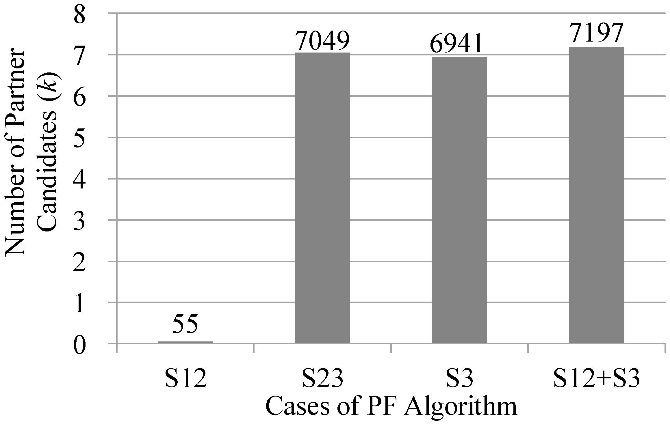
5.2.1. Numbers of Candidate Partners Identified by Different Response Strategies

This experiment analyzed the influence of the response strategy executed on the number of candidate partners identified. As can be seen in the experiment results displayed in Figure 8, the numbers of candidate partners identified by S12 are considerably lower than those identified by the other three strategy combinations. The results of 30 experiments averaged at merely 55 candidate partners. This is because S12 mainly identifies POIs with the same customers as query POI q. However, in the dataset employed in this study (as shown in Table 5), each user only makes about 2 check-ins on average (155,637/81,685 ≈ 2). Therefore, if a customer has already checked in at query POI q, he/she will on average only check in at one other POI. In other words, q can only find a small number of POIs with the same customers, which means that the number of candidate partners that S12 can identify is very low. In contrast, S23, S3, and S12+S3 found substantially more candidate partners than S12 (around 7000 candidates each). This is because with Strategy 3, the algorithm includes all of the POIs in the selected categories as candidate partners. The above results revealed that in most of case (S23, S3), the LBSN dataset no doubt provides more information than can generally be obtained using questionnaire surveys, which also demonstrates the rationality of using LBSN datasets for the proposed recommendation system. Of course, sometimes strategy S12 may face a problem that only few candidate partners are identified, due to the reason that users only leave limited amount of information in the LBSN. Note, however, that in such cases, it should be possible to obtain a reasonable number of candidate partners using other strategies (S12+S3). In the following, we outline an experiment aimed at verifying whether the proposed algorithm can overcome the problems encountered when implementing strategy S12.

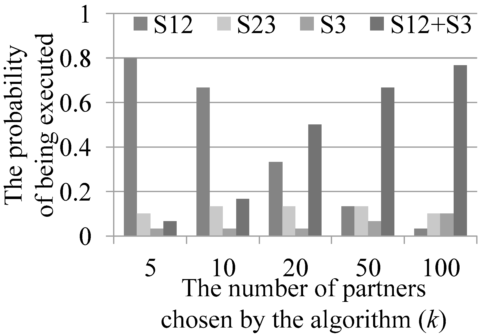
5.2.2. Probability of Each Strategy Combination Being Executed During Queries

In addition to identifying suitable partners, POI owners or managers may also be interested in what promotion strategies they can use. For this reason, we also investigated the probability of each strategy being executed in this paper. Figure 9 shows the results, presenting the probability of each response strategy combination being executed when k = 5~100. First, we found that as k decreases, the probability that S12 is executed becomes far greater than those for S23 and S3. This is because the market circumstances for which S12 is used are common in reality. For instance, q may have only one competitor nearby, with market share ratio of q and the competitor being [1/3, 3] (i.e., Case 3 in Figure 7), or multiple competitors, with q and at least one competitor having a market share ratio within [10/17, 1.7] (i.e., Case 6 in Figure 7). As k increases, the probability of S12 being executed gradually declines, while that of S12+S3 being executed increases to a degree far higher than those of S23 and S3. This is due to the fact that when k increases, the number of candidate partners identified by S12 becomes less than k. This requires that Strategy 3 be executed so that k partners can be identified. When k = 50 and 100, almost all of the cases using S12 required Strategy 3. As a result, the probability of S12+S3 being executed became significantly higher than those of S23 and S3.

In Figure 9, we can also see that in most circumstances, the probability of S3 being executed is lower than that of S23. This is because S3 is only executed when the market share of query POI q is far greater than those of all the other competitors (i.e., Cases 2 and 5 in Figure 7). In practice, this is not common, so the probability of S3 being executed is lower than that of S23 being executed. Finally, we also found that regardless of k, the probabilities of S23 or S3 being executed rarely change. This is because the probability of a strategy combination being executed is only associated with market share and is therefore independent of k. The results above confirm the feasibility of the proposed algorithm in practical applications. Even in cases where strategy S12 was unable to identify a sufficient number of candidate partners to satisfy the query requirements of the POI owner, strategy S3 would be used to cover the discrepancy.

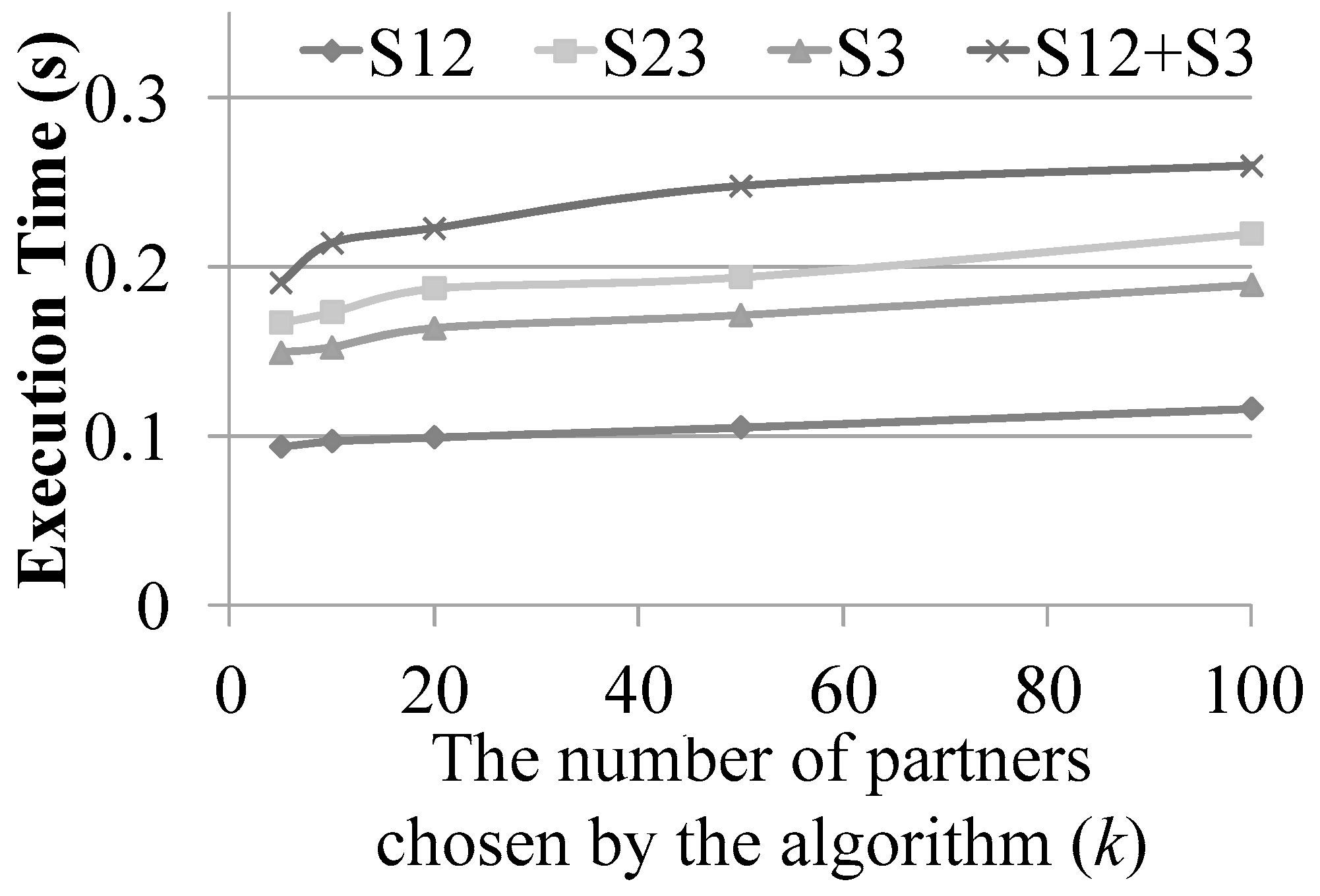
5.2.3. Execution Time of Algorithm Using Various Strategy Combinations

This section discusses the execution times corresponding to the various strategies. The proposed system is intended for online deployment; therefore, it is important to consider the execution time as well as accuracy. The execution times corresponding to the various strategy combinations are presented in Figure 10. Note that for any strategy combination, the execution time falls remained within 0.3 seconds, which falls well within the generally accepted three second standard for webpage query systems. Next, we can see in Figure 10 that the amount of time that the strategy combinations take from least to most is S12, S3, S23, and S12+S3. First, S12 took less time as it identified fewer candidate partners. In contrast, S12+S3 was the most time-consuming because the algorithm must execute S12 and then execute S3, which means it executes the partner search twice.

Both S23 and S3 took more time than S12 because they identified more candidate partners than S12. In terms of S23 and S3 alone, S3 takes slightly less time than S23 because it only needs to find candidate partners from the category graph. S23, however, requires that the algorithm identify not only the POIs that satisfy Strategy 2 in the POI graph but also the POIs that satisfy Strategy 3 in the category graph.

Furthermore, we found that as k increases in Figure 10, the amount of time that each strategy combination takes increases. This is because when k increases, the number of candidate partners that the algorithm must check also increases, which is then reflected in the execution time.

The above experiment results verify that regardless of the requirements of the POI owner, JPPRS is able to return a sufficient number of query results within a short time period sufficient for online implementation.

5.3. Performance Comparison with Baseline Algorithm and Other Relevant Algorithms

In this subsection, we compare the performance of JPPRS with a baseline algorithm and a number of other related algorithms. The baseline algorithm considers only the check-in count of POIs (CC), which is widely used in POI and travel recommendation systems [23, 60]. The other eleven algorithms consider at least one of the partner selection factors mentioned in Section 1. The other algorithms were as follows: shortest distance (SD), demographic data (DA), rating and awareness factor (RA), price and star rating factor (PS), association (AS), POI profile (PP), singularly joint strategy with demographic data (SDA), strategy with rating and awareness factor (SRA), strategy with price and star factor (SPS), strategy with association (SAS), and strategy with POI profile (SPP).We performed two assessments in this experiment: we sought to verify whether the results are relevant to query POI q and how far the identified partners are from q on average. In the real world, POI owners and managers generally do not require a large pool of partners, so we set k = 1~15.

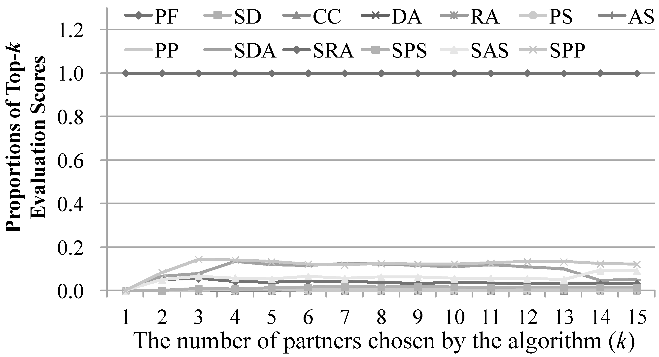
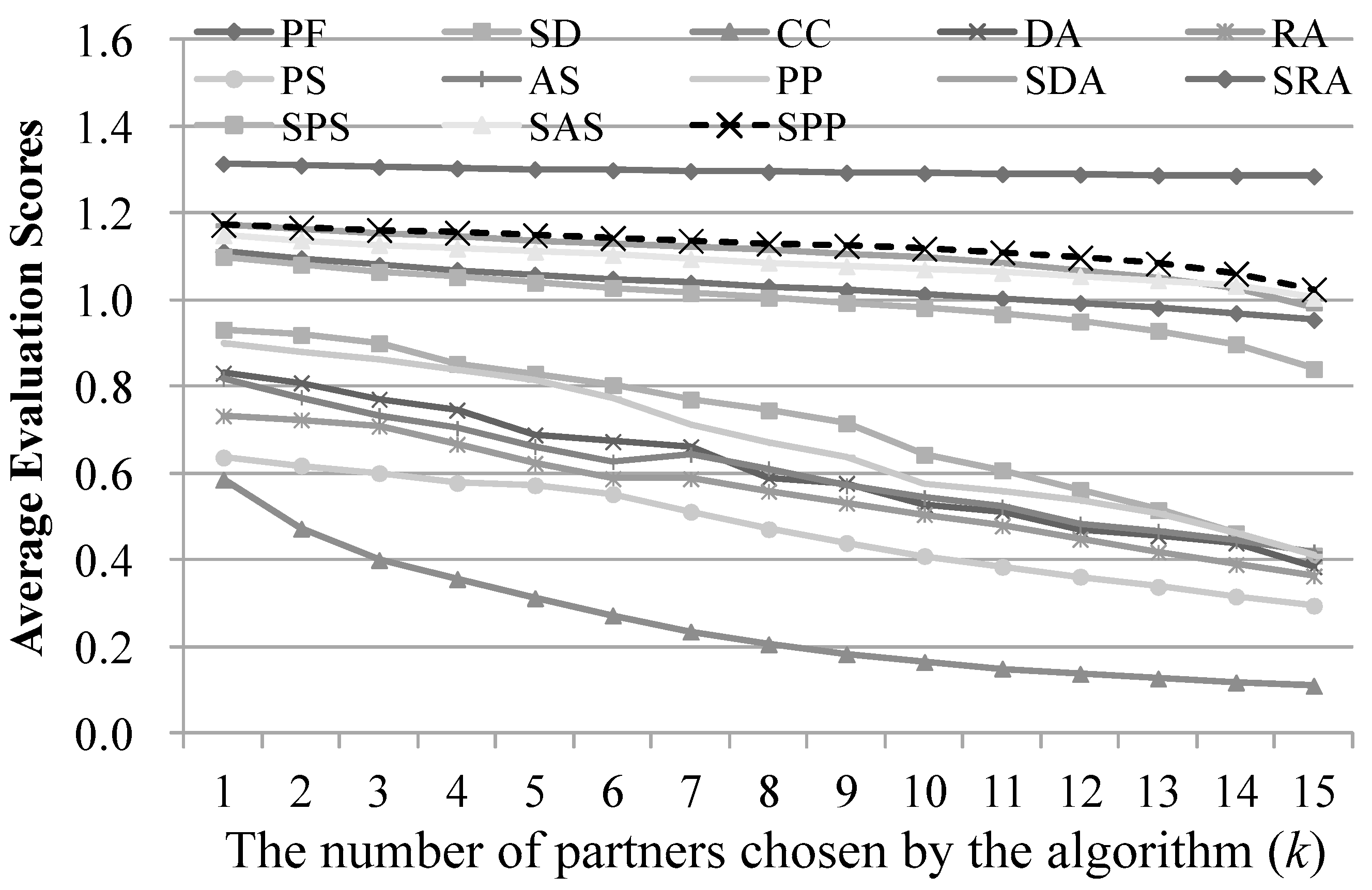
5.3.1. Relevance of Results to Query POI q

In this section, we used an evaluation score and two methods to assess whether the identified POIs are appropriate to query POI q. The evaluation score calculates the suitability of a POI with regard to q and can be written as

$$\mathrm{PS}\left(\mathrm{result}{\left(q\right)}_i,q\right)\times fg\left(\mathrm{result}{\left(q\right)}_i,q\right),$$

(17)

where result(q)_i denotes partner i identified by the methods for q, where 1 ≦ i≦k. PS(result(q)_i, q) is the partner score, of result(q)_i and q, and fg(result(q)_i, q) indicates whether result(q)_i is a POI that the strategy of q is aimed at. If so, then fg(result(q)_i, q) equals 1; otherwise, fg(result(q)_i, q) is 0. If q enters a joint promotion partnership with a POI that does not fit its strategy, the partnership will incur extra costs for q and not attract many customers. In this case, this evaluation score will show that it has no contribution to make to q (i.e., fg(result(q)_i, q)). For each result(q)_i, a higher evaluation score will mean that the POI is more suitable as a partner for q. Using this score, we conducted two experiments to compare our algorithm with the 12 other algorithms. The first experiment determined whether these algorithms can identify the POIs with the top-k evaluation scores for q. The second experiment determined whether the partners obtained by these algorithms have high evaluation scores.

Figure 11 displays the results of the first experiment. In this figure, we can see that for any k, the proposed algorithm derives the POIs with the top-k evaluation scores for q. As for the other methods, they only considered one or two of the partner factors mentioned in Section 1, unlike the proposed algorithm which considers them all. Consequently, they could only find a small portion of the POIs found by the proposed algorithm.

Figure 12 presents the average evaluation scores of the top-k results obtained by our algorithm and the other methods. As can be seen, our method produced the highest average evaluation scores, which indicates that our method is the most capable of identifying suitable partners for query POI q. The other methods could be roughly divided into three groups. The first group included SPP, SDA, SAS, SRA, and SPS, the average evaluation scores of which were slightly lower than our method (PF) because they considered the response strategies and at least one partner factor. The second group contained SD, PP, DA, AS, RA, and PS, the average evaluation scores of which were lower than our method because they only considered partner factors but not the promotional strategies. The final group included only CC, which derived the lowest average evaluation scores of all the methods. This is because POI owners and managers generally do not consider highest popularity when they look for partners. The results in this subsection indicate that the proposed PF algorithm is better suited than other algorithms to finding partners for query POI q, based on the six factors mentioned in this paper. The fact that in any situation, the top-k evaluation scores of PF were higher than those of other methods confirms the effectiveness of the proposed scheme.

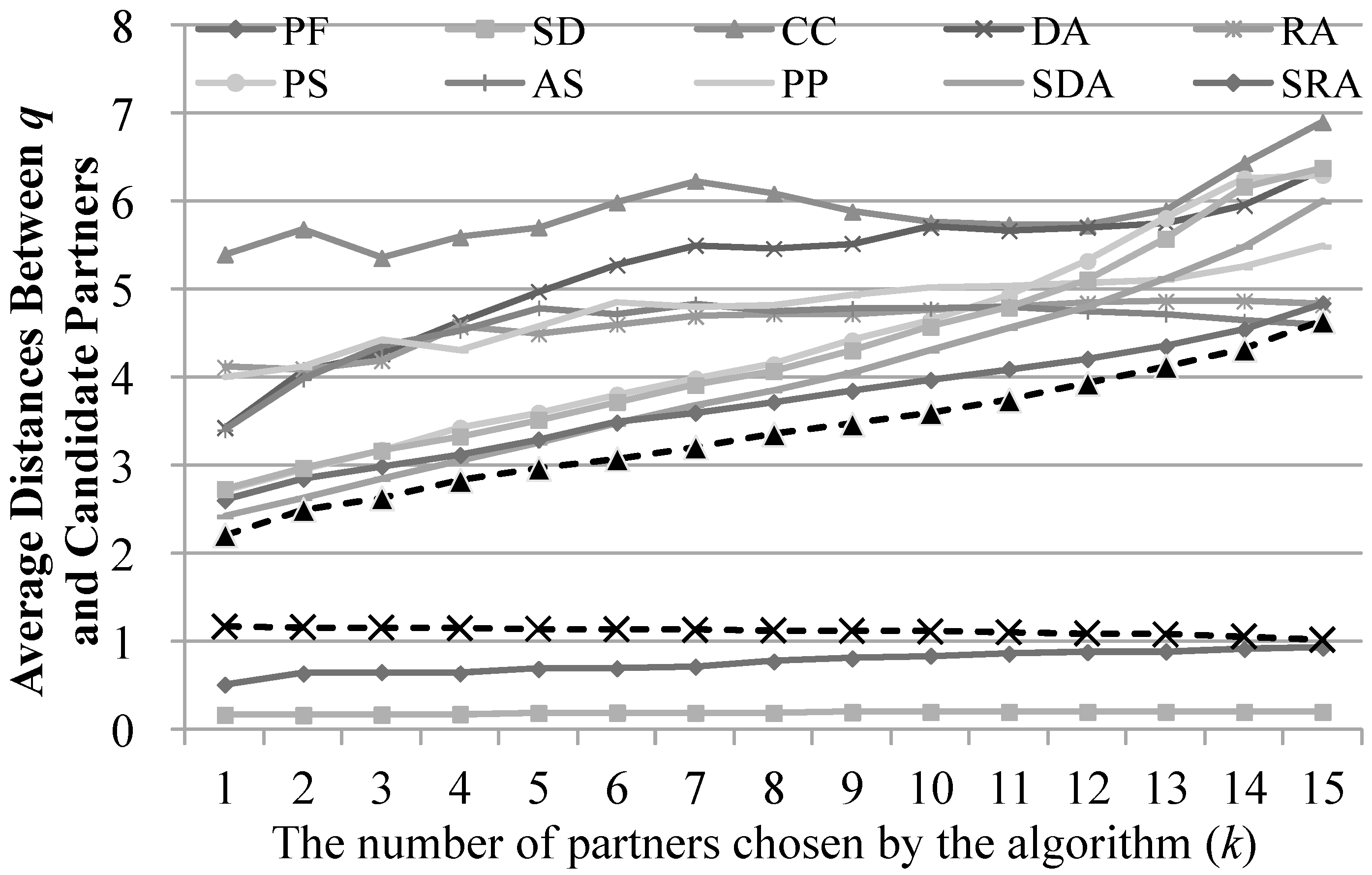
5.3.2. Average Distance between q and Identified Partners

In addition to using the evaluation score presented in the begin of this section to assess the partners identified by our method and the other 12 approaches, we also used distance to determine the suitability of the partners for query POI q. Note that the distance was used here because it is a significant factor affecting the success of joint promotions between two POIs. As we mentioned in Section 1, the shorter the distance between them, the higher the chance of success, and the longer the distance, the higher the chance of failure.

Figure 13 displays the average distances between q and the identified candidate partners. In this figure, we can see that candidate partners identified by the SD approach are on average the closest to q. This is because the SD approach only looked for the top-k closest POIs to q. As can be seen in Figure 13, the average distances derived by our method were larger than those obtained by the SD method; however, regardless of k, the average distances remained less than 1 km. This shows that the proposed algorithm can assist query POI q in finding POIs that are both close to q and suitable partners, which increases the chance of success of joint promotions between q and these POIs. Except for those obtained by SD and our algorithm, we can also see that the average distances derived by the other methods range between 2 km and 7 km, which is several times larger than those from our algorithm. The reason for this was that these algorithms did not take distance into account. If q were to become joint promotion partners with these POIs, the promotion activities would have a smaller chance of success. This is because, a larger distance between two POIs leads to fewer customers who are willing to travel the distance between them. Our analysis in the previous section revealed that the candidate partners identified by the proposed algorithm are not only well suited to query POI q, but also located within 1 km from q.

5.4. Case Study to Verify Accuracy of Our Algorithm

This section uses some actual cases to verify the accuracy of our algorithm. Suppose that in real life, POIs of Category A can cooperate with those of Category B. We therefore performed a top-15 query with the POIs in these two categories, respectively, and compared the two groups of results in terms of recommended categories of POIs.

Table 6. Joint promotion cases.

Category of Query	Category of Partner	Reference
Dry Cleaner	Tailor Shop	[1] p. 37
Tailor Shop	Dry Cleaner	[1] p. 37
Nail Salon	Salon/Barbershop	[1] p. 37
Salon/Barbershop	Nail Salon	[1] p. 37
Cosmetics Shop	Nail Salon	[83] p. 238
Nail Salon	Cosmetics Shop	[83] p. 238
Bakery	Coffee shop, Cafe	[83] p. 186
Coffee shop, Cafe	Bakery	[83] p. 186
Coffee shop, Cafe	Dessert Shop, Snack Place	[83] p. 186
Dessert Shop, Snack Place	Coffee shop, Cafe	[83] p. 186

presents the joint promotion cases that we collected. For the sake of brevity, we limited our discussion here to the combination mentioned in [1]: “A dry cleaning business offers a 50% discount to anyone who visits a nearby tailor. The tailor offers one free hemming service to people who visit the drycleaner. Both businesses benefit from potential new clients and improved relationships with their current customers.”

Figure 14 presents the average results of the top-15 queries performed based on the two only POIs in the dry cleaner category in New York City. The X axis shows the categories that have appeared in the query results. The Y axis on the left measures the average number of times that each POI category appeared in the top-15 queries, whereas the Y axis on the right indicates that average ranking of each category with regard to their appearance in the top-15 queries. Note that the axis on the right presents the ranking in descending order. Because a smaller number generally means a higher ranking, we reversed the order of the axis markings. As can be seen in the figure, the tailor shop category is recommended an average of 1.5 times in the top-15 query results, and each time, it ranks ninth on average, behind the categories clothing stores, women’s stores, and American restaurants. Note that that this is an extremely good result, as there are a total of 425 categories in New York City (as shown in Table 5), but the tailor shop category only falls behind three categories. As for the tailor shop category only appearing an average of 1.5 times in the top-15 query results, which is significantly lower than the 8 times of clothing store, this was because there are only 7 POIs in the tailor shop category in all of New York City, much fewer than the 69 POIs in the clothing store category. The average ranking at ninth place of the tailoring category was also due to the fact that the tailor shops were farther from the dry cleaners than the POIs in other categories were.

Figure 14 also shows that it is more suitable for the two dry cleaners in New York City to partner with clothing stores, women’s stores, and American restaurants than with tailor shops. First of all, clothing stores and women’s stores are not unexpected results as these categories and the tailor shop category are all related to the clothing industry, so they are suitable partners for dry cleaners. The algorithm suggested American restaurants as suitable partners for dry cleaners because the food-related POIs where users check in most frequently (55% of the check-ins in the dataset used in this study were made at POIs related to food and beverage), and the number of POIs in this category is high. As a result, they can often be found near the dry cleaners (i.e., the distances between them and q are shorter), which results in higher partner scores.

Figure 15 displays the average results of the queries performed based on the seven tailor shops in New York City. The axes are the same as those in Figure 14. In this figure, we can see that dry cleaners are recommended an average of 2/7 times. Note that POIs in the dry cleaner category are rarely recommended because there are only two POIs in the dry cleaner category in the New York City dataset; thus, not all of the tailor shops have dry cleaner POIs nearby for the algorithm to recommend. Nevertheless, we discovered that if a dry cleaner appeared in the top-15 results of a tailor shop query, they would always rank fairly high, second on average, which also means that dry cleaner POIs are suitable partners for tailor shop POIs. Figure 15 also indicated that laundry services which are analogous to dry cleaner are also suitable partners for tailor shops. This demonstrates that our algorithm can identify suitable candidate partners in real-world circumstances.

Figure 15 also revealed that in addition to dry cleaners and laundry services, gyms, coffee shops, salons/ barbershops, seafood restaurants, pubs, American restaurants, pizza places, breweries, sandwich places, men’s stores, and nightclubs were also suitable partners for tailor shops. As explained above, POIs related to food and beverages are recommended due to the high number of check-ins at these POIs and high number of POIs in these categories. As for gyms and salons/barbershops, they were likely to be listed by our algorithm as suitable partner categories because they share many of the same customers. This is reasonable because customers who will frequent tailor shops to purchase tailored clothing attach importance to their appearance. It seems likely therefore that they would also frequent gyms and salons or barbershops.

The results for dry cleaners and tailor shops in Figure 14 and Figure 15 confirm that the joint promotion partners identified by JPPRS are similar to those identified using methods based on marketing theory [1].

5.5. Discussion of Experiment Results

The simulations described above confirm that JPPRS provides several advantages over existing schemes. The experiment in Section 5.2 verified that when using the LBSN dataset, JPPRS is able to identify a suitable number of joint promotion partners for a given POI within a suitable period of time. The experiment in Section 5.3 demonstrated the superiority of JPPRS over existing methods in terms of fitness score and distance. The experiment in Section 5.4 verified that the results obtained using JPPRS were very similar to those obtained using methods based on conventional marketing theory [1]. Overall, these results indicate that JPPRS in conjunction with the LBSN dataset is a viable alternative to methods based on marketing theory in terms of accuracy and computational overhead.

6. Conclusions

Joint promotion has been studied extensively; however, much of this work involved field visits, which often involved having participants fill out questionnaires. However, those methods are costly in terms of time and money, and the results are not generalizable. The gradual maturation of LBSN analysis methods in recent years has spawned a wide variety of recommendation systems; however, most of those schemes targeted end-users rather than vendors. In the current study, we developed a novel joint promotion partner recommendation system (JPPRS) based on LBSN data. To the best of our knowledge, no previous works focus on this topic.

In this study, we aimed to create a recommendation system that met the following two conditions: (1) the system had to be suitable for most LBSN datasets, and (2) it had to be directly applicable to a real-world environment. To meet the first condition, we referred to existing studies to select the following six factors common to most LBSNs: customer base, association, ratings and awareness, prices and star ratings, distance, and promotional strategies. To meet the second condition, we designed simple offline and online algorithms with fast calculation capabilities. With these algorithms, the proposed method can be directly realized in the backend of websites, returning results to online users almost instantly. Finally, we used a real-world LBSN dataset to verify the accuracy and efficiency of the proposed system.

This study offers an innovative approach to recommendation systems for businesses and commerce research. The proposed method overcomes the limitations posed by traditional questionnaire-based methods; our experiments verified that using LBSN datasets for analysis can provide better recommendations more swiftly. This paves the way for marketing analysis based on social network datasets. It further pioneers the application of recommendation systems aimed at businesses. The current study is the first to broaden the target of recommendation systems beyond individual consumers. This represents a significant contribution.

Potential future directions of research are diverse. As mentioned, it delves into new topics within recommendation systems such as social network datasets and diverse targets. As such, we focus on a simple framework for practical application within this paper; future research could extend the proposed method in aspects such as data, algorithms, environments, and even application. For example, if system developers could collect more data, more factors could be added to the system to further increase the accuracy of recommendations. System developers could also think outside of the box and go beyond statistical analysis by applying artificial intelligence to make recommendations, which would further enhance the applicability and accuracy of the system. For instance, a rule-based machine learning algorithm could substitute the Lanchester’ law used in this work. A k-means algorithm could be added to categorize all of the businesses in the LBSN beforehand, and then the relationships between categories could be used to estimate the suitability scores of joint promotions between different businesses. Another possibility is application of a deep learning model to learn the characteristics of different businesses to serve as the foundation of searching for joint promotion partners. Considering the sparsity of data in LBSN datasets, a generative adversarial network could also be used to generate reasonable fake data to make up for inadequacies in the LBSN data. In terms of implementation environment, the proposed method was designed with a single host in mind. However, as existing cloud environments are already mature, many recommendation systems also apply the concept of cloud computing to increase computational speed. Regarding application, this study merely considered one-to-one joint promotion partners. Future studies could consider adjusting the proposed method to make it applicable to one-to-many joint promotions or joint promotion alliances.

References

1. Hartnett, R. Small Business, Big Opportunity: Winning the Right Customers through Smart Marketing and Advertising, 2nd ed.; Sensis: Melbourne, Australia, 2008. [Google Scholar]
2. Varadarajan, P.R. Joint sales promotion: An emerging marketing tool. Bus. Horiz. 1985, 28, 43–49. [Google Scholar] [CrossRef]
3. Varadarajan, P.R. Horizontal Cooperative Sales Promotion: A Framework for Classification and Additional Perspectives. J. Mark. 1986, 50, 61–73. [Google Scholar] [CrossRef]
4. Huang, H.C.; Chang, Y.T.; Yeh, C.Y.; Liao, C.W. Promote the price promotion: The effects of price promotions on customer evaluations in coffee chain stores. Int. J. Contemp. Hosp. Manag. 2014, 26, 1065–1082. [Google Scholar] [CrossRef]
5. Kim, W.G.; Lee, S.; Lee, H.Y. Co-Branding and Brand Loyalty. J. Qual. Assur. Hosp. Tour. 2007, 8, 1–23. [Google Scholar] [CrossRef]
6. Chen, H.L.; Huang, Y. The Establishment of Global Marketing Strategic Alliances by Small and Medium Enterprises. Small Bus. Econ. 2004, 22, 365–377. [Google Scholar] [CrossRef]
7. Abowd, G.D.; Atkeson, C.G.; Hong, J.; Long, S.; Kooper, R.; Pinkerton, M. Cyberguide: A mobile context-aware tour guide. Wirel. Netw. 1997, 3, 421–433. [Google Scholar] [CrossRef]
8. Ye, M.; Yin, P.; Lee, W.C.; Lee, D.L. Exploiting geographical influence for collaborative point-of-interest recommendation. In Proceedings of the International Conference on Research and Development in Information Retrieval (SIGIR), Beijing, China, 24–28 July 2011; pp. 325–334. [Google Scholar]
9. Bao, J.; Zheng, Y.; Mokbel, M.F. Location-based and preference-aware recommendation using sparse geo-social networking data. In Proceedings of the International Conference on Advances in Geographic Information Systems, Redondo Beach, CA, USA, 6–9 November 2012; pp. 199–208. [Google Scholar]
10. Logesh, R.; Subramaniyaswamy, V.; Vijayakumar, V.; Li, X. Efficient user profiling based intelligent travel recommender system for individual and group of users. Mob. Netw. Appl. 2019, 24, 1018–1033. [Google Scholar] [CrossRef]
11. Huang, H.H.; Chiu, S.M.; Chen, Y.C.; Lee, C. Group trip recommendation systems. Adv. Intell. Syst. Comput. 2019, 886, 391–412. [Google Scholar]
12. Zheng, Y.; Zhang, L.; Xie, X.; A, W.Y.M. Mining interesting locations and travel sequences from gps trajectories. In Proceedings of the International Conference on World Wide Web, Madrid, Spain, 13–14 January 2009; pp. 791–800. [Google Scholar]
13. DeScioli, P.; Kurzban, R.; Koch, E.N.; Liben-Nowell, D. Best friends: Alliances, friend ranking, and the myspace social network. Perspect. Psychol. Sci. 2011, 6, 6–8. [Google Scholar] [CrossRef]
14. Zhu, J.; Wang, C.; Guo, X.; Ming, Q.; Li, J.; Liu, Y. Friend and POI recommendation based on social trust cluster in location-based social networks. EURASIP J. Wirel. Commun. Netw. 2019, 1, 89. [Google Scholar] [CrossRef] [Green Version]
15. Chen, Y.C.; Li, C.T. Finding potential propagators and customers in location-based social networks: An embedding-based approach. Appl. Sci. 2020, 10, 8003. [Google Scholar] [CrossRef]
16. Kumar, M.S.; Narayana, M.S. A Study on Habits and Preferences of Customers towards Shopping at Modern Retail Stores. Glob. J. Commer. Manag. Perspect. 2018, 7, 7–14. [Google Scholar]
17. Aaker, D.A.; Keller, K.L. Consumer Evaluations of Brand Extensions. J. Mark. 1990, 54, 27–41. [Google Scholar] [CrossRef]
18. Yin, D.; Mitra, S.; Zhang, H. Research Note—When Do Consumers Value Positive vs. Negative Reviews? An Empirical Investigation of Confirmation Bias in Online Word of Mouth. Inf. Syst. Res. 2016, 27, 131–144. [Google Scholar] [CrossRef]
19. Goldsmith, R.; Flynn, L.; Kim, D. Status Consumption and Price Sensitivity. J. Mark. Theory Pract. 2010, 18, 323–338. [Google Scholar] [CrossRef]
20. Hakim, T.; Almahdi, H.K. Impact of Proximity Marketing Devices on Buying Decision-strategical Approach by Small and Medium Size Retail Entrepreneurs. J. Manag. Inf. Decis. Sci. 2020, 23, 187–198. [Google Scholar]
21. Narasimhan, C. Competitive Promotional Strategies. J. Bus. 1988, 61, 427–449. [Google Scholar] [CrossRef]
22. Instagram. Available online: https://www.instagram.com/ (accessed on 29 October 2020).
23. Twitter. Available online: https://twitter.com/ (accessed on 29 October 2020).
24. Facebook. Available online: https://www.facebook.com/ (accessed on 29 October 2020).
25. Flickr. Available online: https://www.flickr.com/ (accessed on 29 October 2020).
26. Dataset Information of Gowalla. Available online: https://snap.stanford.edu/data/loc-gowalla.html// (accessed on 29 October 2020).
27. Foursquare. Available online: https://foursquare.com/ (accessed on 29 October 2020).
28. Gan, M.; Gao, L. Discovering memory-based preferences for POI recommendation in location-based social networks. ISPRS Int. J. Geo-Inf. 2019, 8, 279. [Google Scholar] [CrossRef] [Green Version]
29. Naserian, E.; Wang, X.; Dahal, K.; Alcaraz-Calero, J.M.; Gao, H. A partition-based partial personalized model for points of interest recommendations. IEEE Trans. Comput. Soc. Syst. 2020, Accepted. [Google Scholar]
30. Cao, K.; Guo, J.; Meng, G.; Liu, H.; Liu, Y.; Li, G. Points-of-interest recommendation algorithm based on LSBN in edge computing environment. IEEE Access 2020, 8, 47973–47983. [Google Scholar] [CrossRef]
31. Jiao, X.; Xiao, Y.; Zheng, W.; Wang, H.; Hsu, C.H. A novel next new point-of-interest recommendation system based on simulated user travel decision-making process. Future Gener. Comput. Syst. 2019, 100, 982–993. [Google Scholar] [CrossRef]
32. Kang, L.; Liu, S.; Gong, D.; Tang, M. A personalized point-of-interest recommendation system for O2O commerce. Electron. Mark. 2020, Accepted. [Google Scholar] [CrossRef]
33. Wei, H.; Zhang, H. Research on hybrid recommendation algorithm for integrating consumption habits in LSBN. In Proceedings of the International Conference on Machine Learning and Computing, Shenzhen, China, 15–17 February 2020; pp. 188–192. [Google Scholar]
34. Pan, H.; Zhang, Z. Research on context-awareness mobile tourism e-commerce personalized recommendation model. J. Signal Process. Syst. 2019. [Google Scholar] [CrossRef]
35. Bian, L.; Holtzman, H. Online friend recommendation through personality matching and collaborative filtering. In Proceedings of the International Conference on Mobile Ubiquitous Computing, Systems, Services and Technologies, Lisbon, Portugal, 20–25 November 2011; pp. 230–235. [Google Scholar]
36. Chen, W.; Fong, S. Social network collaborative filtering framework and online trust factors: A case study on Facebook. Int. J. Web Appl. 2011, 3, 17–28. [Google Scholar]
37. Clements, M.; Serdyukov, P.; de Vries, A.P.; Reinders, M.J.T. Using flickr geotags to predict user travel behavior. In Proceedings of the International Conference on ACM SIGIR on Research and Development in Information Retrieval, Geneva, Switzerland, 19–23 July 2010; pp. 851–852. [Google Scholar]
38. Singh, T.; Nayyar, A.; Solanki, A. Multilingual opinion mining movie recommendation system using RNN. In Proceedings of the International Conference on Computing, Communications, and Cyber-Security (IC4S), Chandigarh, India, 12–13 October 2019; pp. 589–605. [Google Scholar]
39. Vesdapunt, N.; Garcia-Molina, H. Identifying users in social networks with limited information. In Proceedings of the 2015 IEEE 31st International Conference on Data Engineering, Seoul, South Korea, 13–17 April 2015. [Google Scholar] [CrossRef]
40. Vicente, M.; Batista, F.; Carvalho, J.P. Gender detection of twitter users based on multiple information sources. Stud. Comput. Intell. 2018, 794, 39–54. [Google Scholar]
41. Vesdapunt, N. Entity Resolution and Tracking on Social Networks. Ph.D. Thesis, Stanford University, Stanford, CA, USA, 2016. [Google Scholar]
42. Asukai, S.; Yamamoto, K. A recommendation system regarding meeting places for groups during events. ISPRS Int. J. Geo-Inf. 2018, 7, 296. [Google Scholar] [CrossRef] [Green Version]
43. Carta, S.; Podda, A.S.; Recupero, D.R.; Saia, R.; Usai, G. Popularity prediction of instagram posts. Information 2020, 11, 453. [Google Scholar] [CrossRef]
44. Guo, D.; Xu, J.; Zhang, J.; Xu, M.; Cuia, Y.; He, X. User relationship strength modeling for friend recommendation on Instagram. Neurocomputing 2017, 239, 9–18. [Google Scholar] [CrossRef]
45. Tiwari, P.; Pandey, H.M.; Khamparia, A.; Kumar, S. Twitter-based opinion mining for flight service utilizing machine learning. Informatica 2019, 43, 381–386. [Google Scholar] [CrossRef] [Green Version]
46. Bao, J.; Zheng, Y.; Wilkie, D.; Mokbel, M. Recommendations in location-based social networks: A survey. GeoInformatica 2015, 19, 525–565. [Google Scholar] [CrossRef]
47. Horozov, T.; Narasimhan, N.; Vasudevan, V. Using location for personalized POI recommendations in mobile environments. In Proceedings of the International Symposium on Applications and the Internet (SAINT), Phoenix, AZ, USA, 23–27 January 2006; pp. 124–129. [Google Scholar]
48. Salter, J.; Antonopoulos, N. CinemaScreen Recommender Agent: Combining Collaborative and Content-Based Filtering. IEEE Trans. Intell. Syst. 2006, 21, 35–41. [Google Scholar] [CrossRef]
49. Barranco, M.J.; Martínez, L. A method for weighting multi-valued features in content-based ltering. In Proceedings of the International Conference on Industrial Engineering and Other Applications of Applied Intelligent Systems, Córdoba, Spain, 1–4 June 2010; pp. 409–418. [Google Scholar]
50. Arase, Y.; Xie, X.; Hara, T.; Nishio, S. Mining people’s trips from large scale geo-tagged photos. In Proceedings of the International Conference on Multimedia, Firenze, Italy, 25–29 October 2010; pp. 133–142. [Google Scholar]
51. Ying, J.J.C.; Lu, E.H.C.; Kuo, W.N.; Tseng, V.S. Urban point-of-interest recommendation by mining user check-in behaviors. In Proceedings of the International Workshop on Urban Computing, Beijing, China, 12 August 2012; pp. 63–70. [Google Scholar]
52. Levandoski, J.J.; Sarwat, M.; Eldawy, A.; Mokbel, M.F. Lars: A location-aware recommender system. In Proceedings of the International Conference on Data Engineering (ICDE), Arlington, VA, USA, 1–5 April 2012; pp. 450–461. [Google Scholar]
53. Liu, Q.; Chen, E.; Xiong, H.; Ge, Y.; Li, Z.; Wu, X. A cocktail approach for travel package recommendation. IEEE. Trans. Knowl. Data Eng. 2014, 26, 278–293. [Google Scholar] [CrossRef]
54. Xie, M.; Lakshmanan, L.V.; Wood, P.T. ComPrec-Trip: A composite recommendation system for travel planning. In Proceedings of the International Conference on Data Engineering, Hannover, Germany, 11–16 April 2011; pp. 1352–1355. [Google Scholar]
55. Hsieh, H.P.; Li, C.T.; Lin, S.D. TripRec: Recommending trip routes from large scale check-in data. In Proceedings of the International Conference on World Wide Web, Lyon France, 16–20 April 2012; pp. 529–530. [Google Scholar]
56. Sang, J.; Mei, T.; Sun, J.T.; Xu, C.; Li, S. Probabilistic sequential pois recommendation via check-in data. In Proceedings of the International Conference on Advances in Geographic Information Systems, Redondo Beach, CA, USA, 6–9 November 2012; pp. 402–405. [Google Scholar]
57. Lu, E.H.C.; Chen, C.Y.; Tseng, V.S. Personalized trip recommendation with multiple constraints by mining user check-in behaviors. In Proceedings of the International Conference on Advances in Geographic Information Systems, Redondo Beach, CA, USA, 6–9 November 2012; pp. 209–218. [Google Scholar]
58. Chiang, H.S.; Huang, T.C. User-adapted travel planning system for personalized schedule recommendation. Inf. Fusion 2015, 21, 3–17. [Google Scholar] [CrossRef]
59. Hosseini, S.; Li, L.T. Point-Of-Interest Recommendation Using Temporal Orientations of Users and Locations. In Proceedings of the International Conference on Database Systems for Advanced Applications (DASFAA), Dallas, TX, USA, 16–19 April 2016; pp. 330–347. [Google Scholar]
60. Hosseini, S.; Yin, H.; Zhou, X.; Sadiq, S.; R, M.; Kangavari, M.R.; Cheung, N.M. Leveraging multi-aspect time-related influence in location recommendation. World Wide Web 2019, 22, 1001–1028. [Google Scholar] [CrossRef] [Green Version]
61. Meng, S.; Wang, H.; Li, Q.; Luo, Y.; Dou, W.; Wan, S. Spatial-Temporal Aware Intelligent Service Recommendation Method Based on Distributed Tensor factorization for Big Data Applications. IEEE Access 2018, 6, 59462–59474. [Google Scholar] [CrossRef]
62. Cai, L.; Xu, J.; Liu, J.; Pei, T. Integrating spatial and temporal contexts into a factorization model for POI recommendation. Int. J. Geogr. Inf. Sci. 2018, 32, 524–546. [Google Scholar] [CrossRef]
63. Ying, Y.; Chen, L.; Chen, G. A temporal-aware POI recommendation system using context-aware tensor decomposition and weighted HITS. Neurocomputing 2017, 242, 195–205. [Google Scholar] [CrossRef]
64. Zheng, X.; Luo, Y.; Sun, L.; Zhang, J.; Chen, F. A tourism destination recommender system using users’ sentiment and temporal dynamics. J. Intell. Inf. Syst. 2018, 51, 557–578. [Google Scholar] [CrossRef]
65. Mukasa, Y.; Yamamoto, K. A sightseeing spot recommendation system for urban smart tourism based on users’ priority conditions. J. Civ. Eng. Archit. 2019, 13, 622–640. [Google Scholar] [CrossRef] [Green Version]
66. Su, C.; Chen, Y.; Xie, X. Location recommendation with privacy protection. In Proceedings of the International Conference on Intelligent Systems, Metaheuristics & Swarm Intelligence, Male, Maldives, 23–24 March 2019; pp. 83–91. [Google Scholar]
67. Huo, Y.; Chenad, B.; Tang, J.; Zeng, Y. Privacy-preserving point-of-interest recommendation based on geographical and social influence. Inf. Sci. 2021, 543, 202–218. [Google Scholar] [CrossRef]
68. Li, W.; Liu, X.; Yan, C.; Ding, G.; Sun, Y.; Zhang, J. STS: Spatial–temporal–semantic personalized location recommendation. ISPRS Int. J. Geo-Inf. 2020, 9, 538. [Google Scholar] [CrossRef]
69. Wang, W.; Chen, J.; Wang, J.; Chen, J.; Liu, J.; Gong, Z. Trust-enhanced collaborative filtering for personalized point of interests recommendation. IEEE Trans. Ind. Inform. 2019, 16, 6124–6132. [Google Scholar] [CrossRef]
70. Mehmood, F.; Ahmad, S.; Kim, D.H. Design and development of a real-time optimal route recommendation system using big data for tourists in jeju island. Electronics 2019, 8, 506. [Google Scholar] [CrossRef] [Green Version]
71. Guo, Q. Graph-based point-of-interest recommendation on location-based social networks. Ph.D. Thesis, Nanyang Technological University, Singapore, 2019. [Google Scholar]
72. Bin, C.; Gu, T.; Sun, Y.; Chang, L. A personalized POI route recommendation system based on heterogeneous tourism data and sequential pattern mining. Multimed. Tools Appl. 2019, 78, 35135–35156. [Google Scholar] [CrossRef]
73. Yang, Y.; Pan, X.; Yao, X.; Wang, S.; Han, L. PHR: A personalized hidden route recommendation system based on hidden markov model. In Proceedings of the Asia-Pacific Web and Web-Age Information Management Joint International Conference on Web and Big Data, Tianjin, China, 12–14 August 2020; pp. 535–539. [Google Scholar]
74. Gao, Y.; Duan, Z.; Shi, W.; Feng, J.; Chiang, Y.Y. Personalized recommendation method of POI based on deep neural network. In Proceedings of the International Conference on Behavioral, Economic and Socio-Cultural Computing, Beijing, China, 28–30 October 2019; pp. 1–6. [Google Scholar]
75. Zhang, C.; Li, T.; Gou, Y.; Yang, M. KEAN: Knowledge embedded and attention-based network for POI recommendation. In Proceedings of the IEEE International Conference on Artificial Intelligence and Computer Applications, Dalian, China, 27–29 June 2020. [Google Scholar]
76. Liu, C.; Liu, J.; Xu, S.; Wang, J.; Liu, C.; Chen, T.; Jiang, T. A spatiotemporal dilated convolutional generative network for point-of-interest recommendation. ISPRS Int. J. Geo-Inf. 2020, 9, 113. [Google Scholar] [CrossRef] [Green Version]
77. Ying, J.J.C.; Lee, W.; Ye, M.; Chen, C.; Tseng, V. User association analysis of locales on location based social networks. In Proceedings of the International Conference on ACM SIGSPATIAL International Workshop on Location-Based Social Networks, Chicago, IL, USA, 1–4 November 2011; pp. 69–76. [Google Scholar]
78. Pan, X.; Hu, R.; Li, D. Social-IFD: Personalized influential friends discovery based on semantics in LBSN. In Proceedings of the International Conference on Communications, Dublin, Ireland, 7–11 June 2020. [Google Scholar]
79. Xin, M.; Wu, L. Using multi-features to partition users for friends recommendation in location based social network. Inf. Process. Manag. 2020, 57, 102125. [Google Scholar] [CrossRef]
80. Luo, C.; Lou, J.G.; Lin, Q.; Fu, Q.; Ding, R.; Zhang, D.; Wang, Z. Correlating events with time series for incident diagnosis. In Proceedings of the International Conference on Knowledge Discovery and Data Mining, New York, NY, USA, 24–27 August 2014; pp. 1583–1592. [Google Scholar]
81. Sarwat, M.; Eldawy, A.; Mokbel, M.F.; Riedl, J. Plutus: Leveraging location-based social networks to recommend potential customers to venues. In Proceedings of the IEEE International Conference on Mobile Data Management (MDM), Milan, Italy, 3–6 June 2013; pp. 26–35. [Google Scholar]
82. Deza, M.M.; Deza, E. Dictionary of Distances; Elsevier Science: London, UK, 2006. [Google Scholar]
83. Mullin, R. Sales Promotion: How to Create, Implement and Integrate Campaigns That Really Work; Kogan Page Publishers: London, UK, 2010. [Google Scholar]
84. Jørgensen, S.; Sigué, S.P. Defensive, offensive, and generic advertising in a lanchester model with market growth. Dyn. Games Appl. 2015, 5, 523–539. [Google Scholar] [CrossRef]
85. Lanchester, F.W. Aircraft in Warfare: The Dawn of the Fourth Arm; Constable and company limited: London, UK, 1916. [Google Scholar]
86. Pearson, D. The 20 Ps of Marketing: A Complete Guide to Marketing Strategy; Kogan Page Publishers: London, UK, 2013. [Google Scholar]
87. Boar, B.H. Constructing Blueprints for Enterprise IT Architectures; John Wiley & Sons, Inc.: New York, NY, USA, 1998. [Google Scholar]
88. Sarwat, M.; Levandoski, J.J.; Eldawy, A.; Mokbel, M.F. Lars*: An efficient and scalable location-aware recommender system. IEEE Trans. Knowl. Data Eng. 2014, 26, 1384–1399. [Google Scholar] [CrossRef] [Green Version]
Figure 1. Example of proposed problem.
Ijgi 10 00057 g001
Figure 2. System framework.
Ijgi 10 00057 g002
Figure 3. An example of age curve.
Ijgi 10 00057 g003
Figure 4. An example of finding a proper distance threshold.
Ijgi 10 00057 g004
Figure 5. Example of POI graph: (a) Visual structure of POI graph; (b) Content of POI graph.
Ijgi 10 00057 g005
Figure 6. Example of Category Graph: (a) Visual structure of category graph; (b) Content of category graph.
Ijgi 10 00057 g006
Figure 7. Different competitive scenarios and response strategies.
Ijgi 10 00057 g007
Figure 8. Numbers of candidate partners with different strategies.
Ijgi 10 00057 g008
Figure 9. Probability of each strategy combination being executed.
Ijgi 10 00057 g009
Figure 10. Execution time of different response strategies.
Ijgi 10 00057 g010
Figure 11. Proportions of top-k evaluation scores among results of various methods.
Ijgi 10 00057 g011
Figure 12. Average evaluation scores of various methods.
Ijgi 10 00057 g012
Figure 13. Average distances between q and candidate partners as derived by various methods.
Ijgi 10 00057 g013
Figure 14. Average results of queries based on the 2 dry cleaners.
Ijgi 10 00057 g014
Figure 15. Average results of queries based on the 7 tailor shops.
Ijgi 10 00057 g015