Prediction of Groundwater Level Variations in a Changing Climate: A Danish Case Study

Abstract

Shallow groundwater is a key resource for human activities and ecosystems, and is susceptible to alterations caused by climate change, causing negative socio-economic and environmental impacts, and increasing the need to predict the evolution of the water table. The main objective of this study is to gain insights about future water level changes based on different climate change scenarios using machine learning algorithms, while addressing the following research questions: (a) how will the water table be affected by climate change in the future based on different socio-economic pathways (SSPs)?: (b) do machine learning models perform well enough in predicting changes of the groundwater in Denmark? If so, which ML model outperforms for forecasting these changes? Three ML algorithms were used in R: artificial neural networks (ANN), support vector machine (SVM) and random forest (RF). The ML models were trained with time-series data of groundwater levels taken at wells in the Hovedstaden region, for the period 1990–2018. Several independent variables were used to train the models, including different soil parameters, topographical features and climatic variables for the time period and region selected. Results show that the RF model outperformed the other two, resulting in a higher R-squared and lower mean absolute error (MAE). The future prediction maps for the different scenarios show little variation in the water table. Nevertheless, predictions show that it will rise slightly, mostly in the order of 0–0.25 m, especially during winter. The proposed approach in this study can be used to visualize areas where the water levels are expected to change, as well as to gain insights about how big the changes will be. The approaches and models developed with this paper could be replicated and applied to other study areas, allowing for the possibility to extend this model to a national level, improving the prevention and adaptation plans in Denmark and providing a more global overview of future water level predictions to more efficiently handle future climate change scenarios.

1. Introduction

Shallow groundwater is defined as the uppermost water table, and is a key resource to human activities and ecosystems [1]. Groundwater is widely used as a source for drinking water (e.g., about 75% of EU inhabitants depend on groundwater for their water supply), is an important resource for industry and agriculture, affects terrestrial ecosystems directly by impacting the vegetation’s access to water, and represents an important link in the hydrological cycle, providing the base flow for surface water systems [2]. Changes in groundwater levels can impact the state of terrestrial and aquatic ecosystems, human health and food provision, and can even pose flooding hazards and cause severe droughts. For instance, several studies have proven that both low and high groundwater levels can negatively impact field crops, with the ideal water table height being between 1 and 2 m below the surface [3,4], and high groundwater levels can intensify the risk of flooding, which might be especially hazardous in urban areas [5].

As global mean temperatures continue to rise, regional patterns of precipitation will be altered [6] and extreme climatic events will occur with higher intensity and frequency [7]. This means that the hydrological cycle will be affected, producing changes in precipitation and evapotranspiration patterns, and altering the periodicity and intensity of climatic events such as storms or droughts [6,8], causing more frequent and severe droughts and flooding events, and affecting the groundwater recharge rates and table elevation [9].

However, these hydrological changes will not be regionally uniform. Different regions have different projections [6], and while some countries will suffer from high reductions in the water table levels and more frequent droughts, countries at higher latitudes, such as Denmark, are expected to potentially raise their water tables due to increases in precipitation and subsequent water recharge rates [10]. For instance, among other changes, it is expected that the water table in Denmark will rise during the wet season due to the increased precipitation, while summers are expected to become drier due to the increase in temperatures and evapotranspiration [11]. Because of the impact and repercussions that these changes in the water level could have, methodologies that can predict the evolution of the water table are growing in importance (e.g., [12,13]). With the ability to model and predict future climate change scenarios and their consequences and impact on both the environment and people’s lives, more and better adaptation plans, as well as prevention measures, can be made.

Machine learning (ML) is a branch of artificial intelligence that focuses on providing systems with the ability to learn automatically from data, improving their decision-making and predictive accuracy over time without being explicitly programmed to do so [14]. ML is increasing in popularity among all fields, and it has been a main component of spatial analyses in GIS, being widely used for classification of spatial components, modelling of spatial varying relationships and predicting changes over time [15].

This increase in popularity can mostly be attributed to the advantages of data-driven models in mitigating the difficulties associated with physics-based models [16,17]; this is, physical relationships and parameters do not need to be defined. ML algorithms only need to process the data, and will find and approximate the relationships between model inputs and outputs through an iterative learning process [18]. Moreover, data availability is improving by the day thanks to the internet, sensors, and improvements in data collection, making ML algorithms a more reliable choice. On the other hand, although ML algorithms are not intended to replace physics-based models, in many cases they have been found to perform better [19], making them a useful and suitable tool for predicting future changes.

Because of the possibilities that ML brings in planning and preparing for future scenarios, these approaches are playing a crucial role in climate change prevention and adaptation. The relevance of ML is thus rising, being increasingly used in modelling the impact of climate change in many fields and from different perspectives (e.g., [12,13]), including the impact that climate change will have on shallow groundwater. Therefore, the aim of this project is to investigate future water level variation under climate change and explore the possibilities of applying machine learning algorithms to groundwater level prediction. Specifically, the goal is to study the potential changes to the shallow water table in Denmark, where current predictions state that groundwater levels will rise due to the increased precipitation that is expected in countries at such latitudes.

1.1. Machine Learning for Groundwater Prediction

With the development of information science and technology, many modelling techniques based on physical principles have been developed and used to explore and understand groundwater dynamics, and to provide quantitative assessments of groundwater resources [20]. These physical models have been widely developed and applied to simulating groundwater dynamics, improving the understanding of hydrologic and water resource systems [21].

The difficulties of applying physical models arise from the fact that it is necessary to develop and solve fluid mechanics and thermodynamics equations, apply detailed boundary conditions, and to describe the dynamics of the hydrological system in order to obtain the input–output relationship. However, solutions for physically based models often require simplifying assumptions because the physiographic and geomorphic characteristics of most hydrologic systems are complicated, and have a large degree of uncertainty in their boundary conditions [22]. Additionally, these models also possess other limitations, such as the requirements on the accuracy of the data or the limitations on the computation resources. Physical models require a large quantity of accurate data, which can never be ascertained with absolute accuracy (e.g., the physical properties of aquifers) [23].

To overcome these limitations that physical models present, more data-driven models based on ML approaches are being studied and applied by researchers as an alternative to physical models [24], and more ML models are being developed for forecasting in various hydrologic research fields (e.g., [25,26]). In the ML approach, physical relationships and parameters do not need to be defined. ML models are data-driven, meaning that ML algorithms only need to process the data, and will find and approximate the relationships between the macro-description of the behaviour of a system (model output) and the behaviour of the constituents of this system (model input) through an iterative learning process [18,27].

Overall, ML models have given very promising results for modelling hydrological systems and dynamics, and for forecasting groundwater levels, in many cases outperforming the results from physical models [19]. Of the many algorithms researched, random forest is being widely used for groundwater modelling, giving very robust results (e.g., [26,28,29]). Different algorithms within neural networks are also widely used for groundwater table forecasting (e.g., [17,30]). Finally, SVMs are also a popular choice and are obtaining good results [31], and usually outperforming other models [23].

For these reasons, this study explores the performance of three ML algorithms when trained with historical groundwater measurements and different geological, topographic, and climatic variables, in order to forecast changes on the depth to shallow groundwater. The selected algorithms are random forest (RF), support vector machine (SVM) and artificial neural network (ANN), based on the information obtained from the literature reviewed.

1.2. Study Objectives and Problem Statement

Current predictions expect Denmark to receive more precipitation in the future due to climate change. With higher precipitation and a rise of temperatures, as well as an increase in the number of sporadic events of very heavy precipitation, the hydrological cycle is expected to be affected by climate change, and local events of flooding, as well as drier soils in the summer, are within the predictions made for Denmark by the Danish Nature Agency. Thus, the water table is expected to suffer changes due to climate change, with increased risks of both floods and droughts.

ML is increasing in popularity as more and more data is available and easily accessible, and this methodology is being increasingly used in forecasting environmental problems and changes including caused by climate change, such as changes in the groundwater levels. Moreover, ML has been proven to be quite efficient for modelling and forecasting changes in hydrology settings, and predictions of changes in the water table will offer better opportunities for the management water resources, by providing adaptation plans for possible events and the risks caused by the change in the water table levels.

Thus, the aim of this study is to gain insights about future water level changes based on different climate change scenarios using ML algorithms while addressing the following research questions:

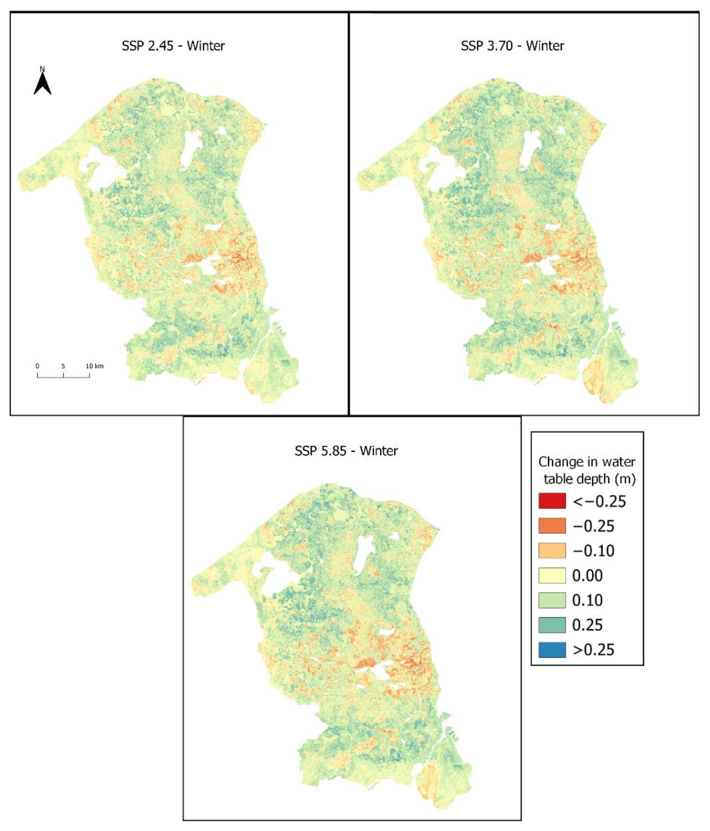
• How will the water table be affected by climate change in the future based on different socio-economic pathways (SSPs)?
• Do ML models perform well enough in predicting changes of the groundwater in Denmark? If so, which ML model outperforms for forecasting these changes?

The major contribution of this study lies within the incorporation of SSPs and advanced machine learning models to predict what the future of water level will look like in the coming decades.

2. Data and Materials

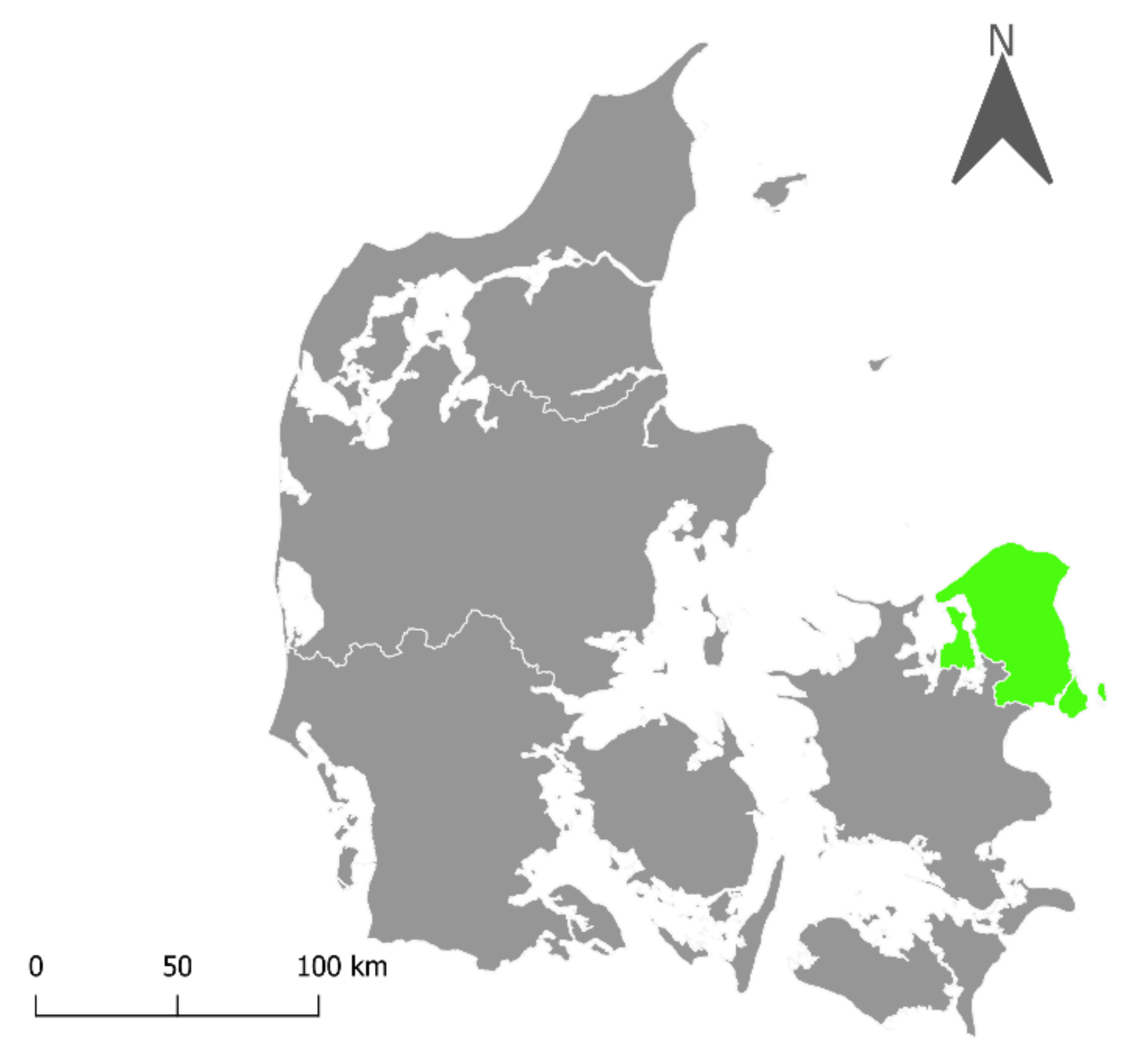
2.1. Study Area

Denmark is a small country with an area of 43,000 km². Basically all of the landscape in Denmark can be labelled as cultural, with barely any pristine nature areas left, since most of the land has been altered. The study area selected, the region of Hovedstaden (Figure 1), comprises 2568 km², of which approximately 43% is agricultural, 39% is urban and less than 20% is natural (forest, wetlands, etc.) [32].

The highest point in Hovedstaden is approximately 96 m above sea level, and the topography is overall modest, with no high elevations and mostly a flat landscape that has been highly modified by glaciers from the Quaternary. Thus, the uppermost sediments are predominantly sandy and clayey tills and sandy or gravelly meltwater deposits that allow groundwater recharge in most areas [33]. These Quaternary sediments cover Tertiary and Cretaceous limestone and chalk, which often hold important groundwater resources in fractures originated from the pressure of past glaciers. The geology is dominated by aquifers based on sandy meltwater deposits and pre-Quaternary limestone, which are covered by a Quaternary clayey till that acts as a confining layer and overlies fractured chalk or limestone. Moreover, as the Quaternary cover is rather thin over the region, the limestone and major aquifers in the study area are vulnerable to pollution [33].

Streams are mainly groundwater-fed and relatively small when compared to other European rivers. The climate in the region is coastal temperate, with average annual precipitation of approximately 700 mm and a mean annual temperature of approximately 7 °C [34]. Due to climate change, the mean annual temperature has increased almost 1.5 °C during the last century, and annual precipitation has increased 15% (100 mm) since 1874, when records began. On the other hand, there are also fewer days of snow cover, with longer warmer seasons and higher rates of evapotranspiration [35].

According to the OECD [35], the projected impacts of climate change in the region show a rise in annual temperatures of 3–5 °C depending on the emissions scenario, leading to fewer days with frost and snow cover. Precipitation will increase 10–40% in winter, and will be reduced in the summer in the order of 10% to 25%, with a clear tendency towards more episodes of extreme precipitation that will yield 20–30% more water than today.

These changes in precipitation and temperature averages will lead to a reduced formation of groundwater in summer and an increased formation during the rest of the year, which will affect the use of groundwater for drinking water or irrigation, and increase the risk of pollution. The Danish water supply relies almost entirely on unpolluted groundwater, so the aforementioned repercussions might lead to limitations on water extraction [11].

Shallow groundwater systems are and will be challenged by climate change. Previous studies have predicted a rise of groundwater levels by up to 1.5 m for a 100-year event relative to present average conditions [36], and climate change will bring changes of at least 0.5 m in the water table for 26% of Denmark [37]. As stated before, changes in the groundwater table levels affect crops and ecosystems, might limit water extraction, and might increase the risk of both local floods and pollution infiltrations to the groundwater [38]. Even though Denmark has abundant groundwater resources, some regions are experiencing pressure on groundwater due to rising temperatures and evapotranspiration [39], and the need for irrigation systems might increase in the future. Therefore, the main concern of these changes on the groundwater table on the region are on the water supply impacts they will cause, from drinking water supply to irrigation issues, while flooding risks are seen as very local hazards that will be mainly caused by heavy precipitation, cloudbursts, and coastal floods from sea level rise [40].

All these problems call for comprehensive modelling tools that can support environmental decision making aiming at tackling current and future challenges related to shallow groundwater.

The region of Hovedstaden was selected due to computational constraints, since the databases were too large for a broader analysis.

2.2. Dependent Variable: Jupiter Database

The depth to water table measurements that were used for this study as the dependent variable were part of a dataset provided by GEUS, called Jupiter. Jupiter is a public national well database with environmental and geotechnical data on groundwater, drinking water, and raw materials [41]. In Denmark, water supply data are reported to the Jupiter database, so the database contains data collected from different companies and organizations in Denmark [42].

The database contains information about more than 280,000 wells, including the technical structure of the wells, geographical location, administrative information, geological descriptions, water level measurements, and groundwater chemical tests and analyses.

This database can be accessed and downloaded as a Postgres database (among other formats) containing more than 100 tables on the different measurements and administrative and metadata on all the wells (more info at [43]).

For this study, the dataset for Hovedstaden was used (available at [44]). It was downloaded as a Postgres database (backup Postgres file) and processed using PgAdmin. The required data, including measurements of the depth to the water table, date and coordinates, among others, were selected in PgAdmin and then connected to QGIS for further processing of the resulting points, clipping them to the extent of the selected study area and exporting them as a shapefile.

Once loaded in R, the measurements were given a proper time format and filtered to a time period between 1990 and 2018. Wells with a screen depth deeper than 10 m were excluded, keeping only measurements for the shallow water table. Outliers were also removed by dropping out measurements deeper than the screen depth, and a maximum of 5 m over the surface was set too. Finally, for wells with several observations in the same month, these daily observations were summarized and transformed into monthly observations. Once this pre-processing was complete, nearly 1200 wells remained, covering more than 10,000 measurements of ground water levels in total, and were then used for training and testing the different ML models.

It is important to note that the number of observations varied greatly from one well to another, some wells had very complete time series while others had fewer measurements of the depth to the water table. Additionally, the available time series were very irregular, as the time frames between measurements varied greatly, from monthly to annual measurements depending on the well, and even changing abruptly in the same well (e.g., from monthly measurements to measurements every other month).

2.3. Independent Variables

In total, 27 variables were acquired for this study, although only 20 of them were used to train the final models (see

Table 1. Data collected for the study. Variables not used for training/testing the final ML models are marked in grey.

Type/Group	Variable	Type	Resolution	Source
Geology	Clay content (1–4)	Continuous	30 m	Adhikari et al. [48]
	Depth to clay occurence	Continuous	30 m	-
	Soil drainage class	Categorical	30 m	Møller et al. [49]
	Soil type	Categorical	N/A	GEUS [50]
Topography	DEM	Continuous	25 m	Copernicus [51]
	Topographic wetness index	Continuous	25 m	-
	Flow accumulation	Continuous	25 m	-
	Slope	Continuous	25 m	-
	Incoming solar radiation	Continuous	25 m	-
Water	Horizontal distance to nearest waterbody	Continuous	25 m	-
	Vertical distance to nearest water body	Continuous	25 m	-
	Water bodies (lakes, streams, etc.)	Categorical		Koch et al. [29]
	Sea level	Continuous	N/A	NOAA [52]
Land cover	Corine	Categorical	100 m	Copernicus [53]
	Imperviousness	Continuous	20 m	Copernicus [54]
Bioclimatic variables (monthly historical data)	Precipitation	Continuous	4.5 km	Harris et al. [55]
	Minimum temperature	Continuous	4.5 km
	Maximum temperature	Continuous	4.5 km
	Average temperature	Continuous	4.5 km
Coordinates	xytm	Continuous	25 m	-
	yutm	Continuous	25 m	-
Bioclimatic variables–Future projections	Precipitation	Continuous	4.5 km	Fick & Hijmans [56]
	Average temperature	Continuous	4.5 km

). The data used for this study were chosen following the recommendations from the literature [29,45,46,47]. Some of the variables could be obtained from different sources, while others had to be calculated.

The clay content was developed by Adhikari et al. [48] and the dataset was composed of four tif files, each showing a different depth level of the soil. In this way, clay 1–4 represent the content of clay as a percentage in the first 0–30, 30–60, 60–100 and 100–200 cm of soil, respectively. The depth-to-clay ocurrance was calculated in R by using available soil types and their depths, provided by a local consulting company. Thus, the depth to the clay layers of soil was used to obtain a single layer with the total depth to the first clay occurance, in metres.

The soil drainage class was developed by Møller et al. [49]. It consists of a tif raster file with categorical values from 1 to 5 depending on the drainage class of the soil, with 1 being very well-drained soils, while 5 being very poorly drained soils.

The soil type was obtained from GEUS, and it was a shapefile containing the different types of soils as polygons. This shapefile was transformed to raster in R. More information about the different soil categories can be read at the source [50]. The horizontal and vertical distance to water bodies were both calculated in SAGA by using both the digital elevation model (DEM) and the water bodies files. Additionally, the topographic wetness index (TWI), flow accumulation, slope and incoming solar radiation for each month of the year were also calculated in SAGA using the DEM.

Finally, the DEM, imperviousness and Corine land cover were all obtained from Copernicus as raster files, while all the climatic variables, both historical [55] and future predictions [56], were obtained from WorldClim. The reason to choose this historical climate data was the available temporal resolution, as no other datasets were found that covered the period selected for this study in monthly measurements. Similarly, the Corine land cover and Copernicus imperviousness data also had a rather suitable temporal scale, covering several years during the selected period, and thus changes on both land cover and imperviousness could be considered.

Future projections for the bioclimatic variables were available for several periods of time and four different socio-economic pathways (SSPs). For this study, the future projections were selected for the period 2060–2100, along with the SSPs that follow best current EU and Danish plans and legislation regarding gas emissions. Thus, the selected SPPs were SSP2-4.5 (a scenario where efforts are made to limit warming to 3 °C by 2100, with a slow decline of CO₂ emissions), SSP3-7.0 (a middle of the road scenario showing 4.1 °C of warming) and SSP5-8.5 (a high-emission business as usual scenario with a mean warming of 5 °C).

Further pre-processing of the data was performed in RStudio. All the data were reprojected to a Danish projection system (EPSG:25832) and resampled to a resolution of 25 m by the nearest neighbour method. This method ensures that no new values are created when resampling the data, which is especially important for categorical variables like land cover, as new values do not account for any of the categories established for this dataset. Finally, the data was all clipped to the extent of the study area and exported as tif files that were later used for training the models and for the predictions.

3. Methods

3.1. Machine Learning Algorithms

In this project, regression ML was used by using the Caret package [57] in R. Regression analysis consists of a set of machine learning methods that allow us to predict a continuous variable (y) based on the value of one or multiple predictor variables (x) [58]. The goal of this methodology is to build a mathematical equation which defines y as a function of the x variables, and then use the equation to predict the outcome (y) based on new values of the predictor variables (x).

3.1.1. Random Forest

Random forest (RF) is an ensemble of decision tree (DT) algorithms, first developed by Breiman [59]. Decision tree is a supervised learning algorithm used for both classification and regression problems, and the RF algorithm is an extension of a bootstrap aggregation of DTs. The RF algorithm constructs multiple DTs that are trained in parallel with random bootstrapped samples of the training dataset, using different subsets of available features [59]. This method ensures that each DT is unique, since each is fit on a slightly different training dataset, thus showing a slightly different performance and reducing the variance of the RF. For the final prediction, all the predictions from the individual trees were aggregated and averaged, resulting in better performance than any single tree in the model [60].

This method also allows the RF to predict the importance of the variables by examining how much of the error of prediction increases when one of the variables is left out (out of the bag, oob) while the rest are left fixed [61].

For tuning the RF, the hyperparameters to consider are the number of trees (ntree) and the number of variables randomly sampled as candidates at each split (mtry).

3.1.2. Artificial Neural Networks

ANNs are pieces of a computing system designed to simulate the way the human brain analyses and processes information. ANNs are built up with hundreds or even thousands of artificial neurons which are called processing units, which are interconnected by nodes [62]. These nodes can be weighted to communicate each one’s strength and affect the final model outputs. The weights of these nodes are combined before being passed through an activation function that ultimately translates the input into an output with a value range of 0–1, in a process called feed-forward [63].

ANNs also use a set of learning rules called backpropagation or backward propagation of error. ANNs go through a training phase where they learn to recognize patterns in data, in which where the network compares the output with the actual measurements or what it was supposed to be. The difference between the outcomes is then adjusted using backpropagation, meaning that the network goes backwards from the output to the input units to adjust the weight of the connections between the units until the difference between outcomes produces the lowest error possible [62].

The hyperparameters that are necessary to tune for ANNs in the caret package were the decay, which is the regularization parameter to avoid overfitting, and the size, which serves to adjust the number of units in the hidden layers.

3.1.3. Support Vector Machines

Support vector machines are a set of supervised ML methods used for classification, regression and outlier detection. SVMs use a binary or multi-class approach to data segregation, finding a hyperplane that maximizes the margin between the classes of the data. The vectors that define the hyperplane are the support vectors. In the case of regression problems, a margin of tolerance is approximated, but the idea is the same: to minimize the error by individualizing the hyperplane that maximizes the margin.

SVMs are effective in high dimensional spaces, even in cases where the number of dimensions is greater than the number of samples. SVMs are also versatile, as they can be used for both linear and non-linear data by applying different Kernel functions to the decision function of the support vectors. However, SVMs are negatively influenced by large, noisy datasets, proving less suitable for these types of datasets than other ML algorithms [64].

When tuning a SVM model, the hyperparameters used are c (cost), which controls training errors and margins, and sigma, which determines the reach of a single training instance.

3.2. Implementation

First of all, the groundwater data was pre-processed as explained in Section 2.2., while the independent variables were all loaded into R and pre-processed to have the same extent and resolution, as explained in Section 2.3.

Once all the data were pre-processed in R, the extract function from the raster package [65] was used to get the background data for each of the groundwater observations at each of the observations’ location, and according to the date when they were collected. Like this, monthly precipitation and temperature were linked to each observation by date, and imperviousness and landcover were also extracted according to the year. The result of this process was a dataframe containing the groundwater measurements for each well along with the corresponding background data for each observation.

After the background data were extracted, the next step was to perform a PCA and a correlation test to better understand the importance of the different variables, excluding those that were highly correlated or explained little of the variation of the data, in order to reduce noise and avoid overfitting of the ML models. First, the correlation test was performed to detect collinearity between the variables by using the cor function built into R, and corrplot was used to see the correlation matrix. The correlation matrix shows the pairwise correlation between variables, both positive (blue) and negative (red), showing a stronger correlation with darker colours and bigger circles (Figure 2).

By examining the correlation matrix (Figure 2), it is easy to detect a strong positive correlation between the temperature variables, and some correlation between the temperature variables and incoming solar radiation (ins), especially with the maximum temperature (tmax). The Pearson correlation coefficient was also calculated separately, and a threshold of ±0.70 [66] was applied for the correlation coefficient, excluding variables that were highly correlated. It was decided to keep the average temperature (tmean) in order to have a bigger overview on the variance between minimums and maximums, and also because the maximum temperature showed the highest correlation to incoming solar radiation.

Then, a PCA was performed to determine how much of the variation of the data was explained by each of the independent variables, thus finding their importance in order to exclude the least important ones. Since PCA cannot handle categorical variables well, this process was performed only with the continuous data, leaving land cover, drainage class and type of soil out of the analysis. The PCA was performed with the function prcomp which is built into R, and factoextra was used to visualize the results. In the final graph obtained (Figure 3) the contribution of each variable to the first and second PCs, which are the ones explaining most of the variation of the data, can be seen.

After performing the PCA, the flow accumulation and sea level variables were also excluded, as these added little to the main PCs. The PCA also showed that both precipitation and temperature were quite low in the contribution to the first and second PCs, although their contribution was higher in following PCs. Additionally, these climatic variables are the ones with the highest variation as they are historical monthly data, while the other variables are mostly static, so these two were kept in the analyses. The PCA does not really examine the relationship between the independent variables and the values of the dependent variable, while RF and ANN do, when analyzing the importance of the variables. Therefore, these variables were left in the analyses for the models to pick up their importance, as they are supposed to be relevant for changes in the water level and thus, for forecasting future scenarios where these variables will undergo large changes. After dropping the highly correlated variables and those that explained little of the variation of the data, 20 independent variables were used for the models (see Section 2.3.).

For hyperparameter tuning, the caret package can optimize the hyperparameters for each model by using a random search and selecting the optimal values for each of the hyperparameters. This method allows it to easily find the best hyperparameters for each model, while making it possible to build all the models in a similar fashion so they can be compared easily. To train the models with caret, it is necessary to input the independent variables as a dataframe and the dependent variable as a vector separately, and some parameters need to be set: Method is used to set the ML algorithm to be used; trainControl defines the type and number of resampling, as well as the search method (for this project, a 5-fold cross-validation was used); metric determines how the final model is defined by selecting the tuning parameters with the highest value of the objective function (since these are regression models, it was set to “Rsquared”); and tuneLength sets the size of the default grid of the tuning parameters (it was set to 10 for all the three models).

The parameters were selected according to the literature and by trial and error when setting the models. For reproducibility, a seed number was set before each model. After setting all the parameters, the models were run, and the following performance metrics for each model were obtained: coefficient of determination (R2), mean absolute error (MAE) and root-mean-squared error (RMSE).

These metrics are used in regression ML models to assess the goodness of fit of the model and are obtained internally by the caret package when each model is run, summarizing the divergence between actual, observed data points and the expected data points for each ML model. In a regression ML model, R2 represents the proportion of variance of the dependent variable that has been explained by the independent variables in the model. It is an indication of goodness of fit, providing a measure of how close the observed data points are to the predicted points, showing how much of the variance contained in the training data is captured by the ML model. If $\widehat{y_{ }}$ is the predicted value of the i-th sample and y_i is the corresponding true value for total n samples, the estimated R² is defined as:

$$R^2=1-\frac{{{\displaystyle \sum }}_{i=1}^n{\left(y_i-\widehat{y_i}\right)}^2}{{{\displaystyle \sum }}_{i=1}^n{\left(y_i-\overline{y_i}\right)}^2}$$

The MAE is expressed as the average of the absolute values of the differences between the predicted and the actual values, and a form of verification of regression ML models. The MAE can be defined as:

$$MAE=\frac{1}{n} {\displaystyle \sum }_{i=0}^{n-1}{\left|y_i-\widehat{y_i}\right|}^{ }$$

where $\widehat{y_{ }}$ is the predicted value of the i-th sample, y_i is the corresponding true value, and n is the total number of samples or errors.

Finally, the RMSE is a measurement of the model’s prediction error, being a quadratic scoring rule which measures the average magnitude of the error. The RMSE is computed as:

$$RMSE=\sqrt{\frac{{{\displaystyle \sum }}_{i=1}^n{\left(y_i-\widehat{y_i}\right)}^2}{n}}$$

where $\widehat{y_{ }}$ is the predicted value of the i-th sample, $y_i$ is the corresponding true value, and n is the total number of samples or errors.

Since the RF model was the one with the best outcome, three more RF models were also trained based on three different land cover types. Thus, 3 models were trained by dividing the data into three categories: nature, agricultural and urban. This was done to check whether the location of the wells affected the model, or if the placement of the wells was affecting the observations.

Because static variables can cause overfitting in these types of models [67], additional RF and ANN models were trained, excluding all non-climatic variables to determine if the static variables were in fact overfitting the models. However, the results of this technique were not good, and further analyses on this matter were dropped.

For the future predictions, data for the different climate scenarios for both winters and summers were used. However, not all the data were available for the future climatic scenarios. For instance, climatic data were available for all the three different SSPs selected, but future predictions on land cover and imperviousness were not available. Therefore, the latest available data for these variables were used, which accounted for the period 2018–2020.

The variables for the different SSPs were pre-processed following the same steps as for the predictors used to train the models. This data were added to R as a raster stack and used with the predict function from the raster package along with the first trained RF model, as this was the one with the best results. Two predictions were made for each of the SSPs selected (SSP2-45, SPP3-70, SPP5-85), one for the winter and one for the summer.

The exact procedures in R can be seen in the code developed for preprocessing the data and building the ML models, which is available in the supplementary materials.

The resulting maps obtained from the predictions were exported as tif files and further processed in QGIS for better visualization and to make the final maps.

4. Results

The following section is used to show and describe the results obtained from the ML algorithms, starting with the direct metrics obtained from the ML models, and finishing with the prediction maps developed with the selected ML model.

4.1. Comparison of the Models

As explained in the implementation section, after performing the PCA and the correlation test, four variables were excluded for being too highly correlated or for explaining too little of the variation of the model, and further training of the models was performed without them.

After training the three different models and obtaining their performance metrics, it can be seen that the RF model was the one with the better scores (

Table 2. Result scores obtained from the training of the three different models.

ML Model	R2	RMSE (m)	MAE (m)
RF	0.75	0.98	0.61
ANN	0.63	1.19	0.85
SVM	0.65	1.15	0.75

), obtaining the highest R² (0.75) and the lowest MAE (0.61 m) and RMSE (0.98 m) of the three.

In the caret package, both RF and ANN have a built-in mechanisms to report on variable importance. When examining the importance of each variable based on these models (Figure 4), static variables like the elevation (dem), horizontal and vertical distance to water bodies (hdistance and vdistance, respectively) or the depth to clay ocurrance (cly_dpt) had relatively high importance in both models, being the predominant factors explaining the variation in the groundwater data. Imperviousness (imperv) also had a rather high importance in both models, while precipitation and temperature were, surprisingly, quite low, especially in the ANN model.

These results also go along with the PCA performed, where the climatic variables had a rather low importance in the first two principal components. No results are shown for the SVM, as this model does not have a built-in function to account for variable importance.

Three more RF models were trained with wells located in different land cover types. When dividing the data by land cover, three land cover types were used: urban, agricultural and nature, to determine whether the location of the wells affected the predictive efficiency of the model (

Table 3. Scores for the RF models trained with data from different locations based on land cover.

Land Cover Type	R2	MAE (m)
Urban	0.70	0.63
Agricultural	0.65	0.69
Nature	0.86	0.38

).

After training the three models with RF, it can be seen that the model seems to perform best on natural areas, while the worst performance seems to be in agricultural areas, which might indicate that there were other factors apart from the variables used in the model affecting some of the observations. However, it is also important to note that the number of observations in natural areas was lower than those of either the urban or agricultural land cover types.

Another reason for having least accuracy in farms would be that farms’ moisture level is manipulated through irrigation and the planting of high water consumption crops. Moreover, these crops are not planted every few years for maintenance purposes and hence the water level variation changes naturally. This means that farmlands are sometimes actual agricultural crops and sometimes are left as grass/barren land, depending on the region [68,69].

A RF model without any of the static variables was also trained to account for a possible overfit in the model caused by these factors. As explained before, land cover and imperviousness were also treated as static because they changed little during the period selected for this project. Therefore, only precipitation and temperature were used for this model.

However, the results were unsatisfactory, with low metrics after training (R² of 0.39 and MAE of 1.31), showing a very low predictive power. Thus, it seems that although the static variables can overfit a model, they also to some extent explain the variation of the data.

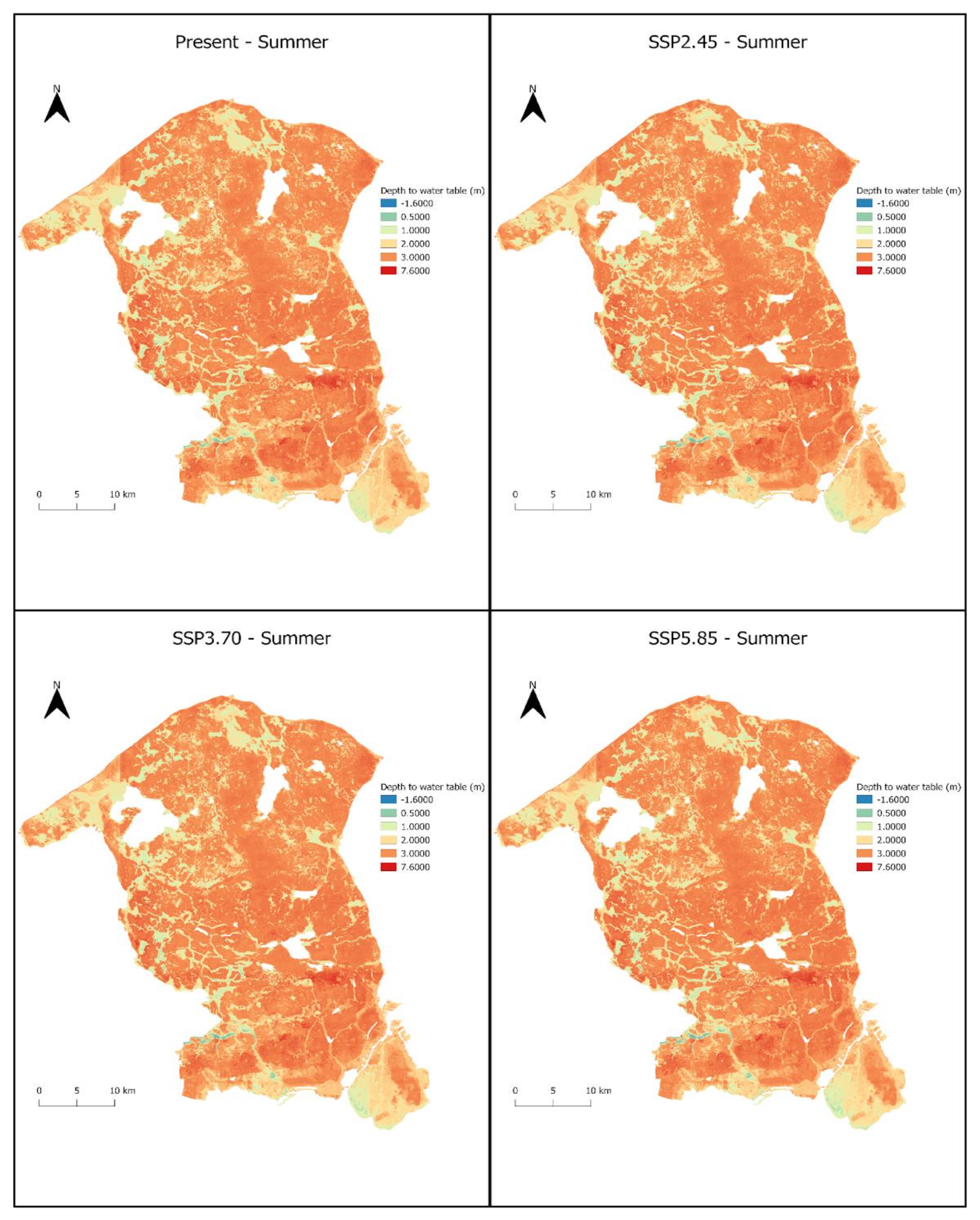
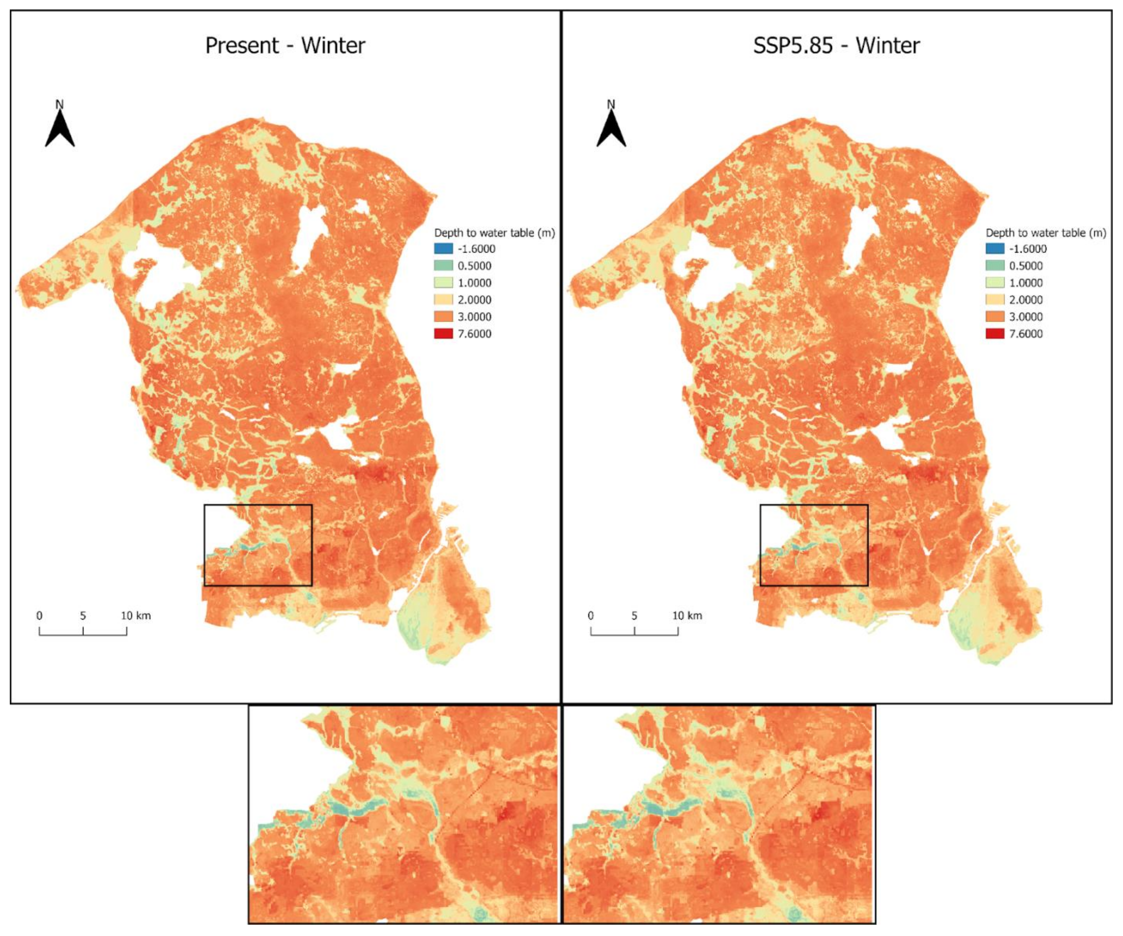
4.2. Future Predictions

Two prediction maps for each of the climatic scenarios were obtained from the predictions made with the RF model, one for the winter season and one for the summer season. Additionally, two maps were also obtained for the current situation, one for winter and one for summer. The final maps for each season and each climatic scenario can be seen in Appendix A.

Visually, there were no noticeable changes between climatic scenarios, although differences between the present and future water levels can be noticed, especially in some specific areas like to the east of Copenhagen (an example can be seen on Appendix A, Figure A1 and Figure A2). The maps show that, overall, the future water table will be higher, both in winter and summer, with the SSP2.4-5 being an exception by having levels similar to the current situation. Additionally, it shows that summers will be drier than winters, in line with the expectations from the literature [29].

Comparing a specific area in present and future scenarios (Example available in Appendix A, Figure A3), it can be appreciated that the orange and red shades were lighter in the future scenarios, and there were more blue shades, meaning that the groundwater will be closer to the surface in a larger area (

Table 4. Comparison of the % of groundwater in the first meter from the surface.

Scenario	Winter (%)	Summer (%)
2018	1.40	1.26
2.4–5	1.40	1.25
3.7–0	1.43	1.29
5.8–5	1.43	1.41

).

The average groundwater levels of the different scenarios oscillated between 2.95 and 3 m, being rather stable over the study area regardless of the month and scenario. However, when considering how the groundwater levels are distributed, we can see that in future scenarios there is an increase in the areas where the water table will be closer to the surface, even in the summer periods. Since the first meter from the surface is the most important, as the water table at this depth highly affects the surface, 1 m was the focus for showing changes to the water table depth.

The differential maps obtained between present and future scenarios (Figure 5 and Figure 6) show that overall, water levels will rise during the winter, while in the summer months most of the area will remain the same (yellow shades) or suffer a slight decrease (orange shades), although several areas will also see a raise in the water table (green/blue shades). In both cases, changes will still be limited, and most of the area will suffer changes within 0–0.25 m. While it could be seen before that the first meter of soil will overall be impacted by a rising water level (Table 4), it seems that the water at deeper levels will fall in summer, although not much (between 0 and 0.25 m).

When further studying these comparisons between the different future scenarios and the present, we can see that the fluctuation in the maximum rise values for the water levels were larger than the maximum fall values (

Table 5. Maximum change in the water level (rises and falls) for each of the scenarios compared to the present levels for both winter and summer.

	Winter			Summer
Scenario	SSP 2.4-5	SSP 3.7-0	SSP 5.8-5	SSP 2.4-5	SSP 3.7-0	SSP 5.8-5
Max. rise (m)	+0.67	+0.83	+0.82	+0.70	+0.70	+0.71
Max. fall (m)	−0.52	−0.47	−0.49	−0.52	−0.49	−0.52

), and that the increase in the maximum rise values was especially noticeable in the scenarios with higher emissions (especially during the winter).

When examining these results, it should be noted that, since the model is based on water levels from wells with no observations of either streams or water bodies, the model seems to predict drier scenarios than what should be expected, and the groundwater in streams is not represented over the surface. These limitations, together with the aforementioned possibility of overfitting, should be taken into consideration when inferring conclusions based on the model predictions.

5. Discussion

5.1. Comparison of the Models

RF had the best metrics in both the training and testing sets, and was, for this reason, deemed best for further analyses and for this project. As reviewed in the literature, RF is a model widely used in hydrology settings such as groundwater level forecasting, and it has been proven to provide very robust results and accurate predictions in several studies (e.g., [26,29,45]).

Although ANN and SVM are also popular choices in this field, they were outperformed by the RF model in this project. Even though it is a possibility that the tuning of these two models was insufficient because our goal was more focused on allowing comparison between the three models, it is not uncommon for RF to outperform models such as ANN [70]. Thus, with the data available for this project and with the tuning possibilities researched for each model, it can be concluded that the best model was RF, followed by ANN and finally SVM.

As was mentioned before, there is a possibility of the models being slightly overfit. As a measure to improve the model, possible overfitting was accounted for and different steps were followed to attempt to reduce it. As seen in the literature, it is possible, in models that use spatio-temporal data, to get overfit when static variables are used [63]. However, removing those static variables from the model did not improve the results, which might mean that the climatic variables alone were insufficient to predict changes in the groundwater level in the study area.

Additionally, an attempt was made to divide the groundwater data by season, as having a single model with data for both wet and dry seasons was presumed to be too confusing for the model. But this division of the data into wet and dry seasons did not improve the results either, giving similar metrics and predictions to those already obtained with the original RF model. Therefore, this approach was disregarded and, due to resource and time constraints, was not further investigated.

However, this should not reduce the value of the results from the RF model, since the metrics of the model are within the expectations for a successful model [71].

5.2. Future Predictions

According to our results, even though there were slight differences in the water levels amongst the different present and future scenarios, there seems to be less fluctuation than expected [36] in these values according to the selected RF model, based on the data available to apply. There are different reasons that could explain this limited change.

On one hand, artificially drained areas are not expected to have a rise in the water table depth, but rather the increase in precipitation will cause an increase in the drainage water runoff [72]. The selected study area is highly anthropomorphic, being composed of mostly agricultural and urban areas, and it is likely that artificial drainage in the region is extended throughout the area, although information on this specific factor could not be found for this project. Therefore, it is possible that the water table in the region will not suffer major changes.

On the other hand, both precipitation and temperature are expected to increase in the future, which would translate into a higher water level due to higher recharge rates as a result of precipitation, and also into a lower water level due to increased evapotranspiration caused by the rise in temperatures [11]. Because of these two opposite effects taking place, it is possible that average water levels for long periods such as dry and wet seasons, as compared in this project, will not change much in the future.

Additionally, the model picked some static variables as being important in explaining the variation of the water level. Since these variables will not change for each well for the different future scenarios, it is reasonable that there would just be small changes between their groundwater levels.

Regardless of the small changes in the average groundwater levels, it can be seen that in future scenarios (especially for the scenarios with higher emissions), the water table will be closer to the surface in some areas, albeit sometimes only barely so. Still, even small changes to the water table in the first meter of the terrain can greatly impact the ecosystems and human activities on the surface [4], and close attention should be paid. This is especially relevant when considering that the water table rising closer to the surface would translate into a higher risk of flooding, especially in case of heavy precipitation events [29]. It is highly possible that the risk of flooding will be very local, and specific to certain events such as heavy storms events [40].

It is expected that sporadic precipitation events will be more common and increase in intensity in the future in Denmark [11]. These sporadic events are not considered in the average precipitation data used in the model. The model presented in this paper is not trained to pick up on these extreme scenarios; it simply draws an overall trend based on how the groundwater levels have changed month-by-month, and how they will change based on the climatic changes in the future. For this reason, any raise, even if small, should be monitored closely, since any raise in the average groundwater level of an area estimated by the model could actually mean much more significant rises during these extreme scenarios, translating into possible flooding or pollution infiltration scenarios.

Current concerns regarding the groundwater in Denmark are mostly focused on possible pollution infiltration to the groundwater, as it is a valuable resource for water supply [35,38]. Changes in the water table levels can increase the risk of pollution of the groundwater, as pollutants infiltrate through the soil and come in contact with the water [72]. In addition to this, there are other concerns regarding the effect that a higher water level will have on artificial infrastructures such as sewers, water pipes or buildings. If the groundwater level rises, it will result in increased pressure on the foundations of buildings that are below the groundwater level. Moreover, groundwater can infiltrate through leaks in sewer and water supply pipes, and pollutants in the soil can infiltrate into the pipes with the water [73].

5.3. Limitations of the Model

As mentioned before, there are multiple factors that should be taken into consideration when inferring conclusions based on model predictions. The fact that the studied region is so affected by human activities could impact the ML model predictions. These areas are susceptible to water table modifications due to artificial drainage and irrigation, which are factors that the current model is not considering, and that might in turn be affecting the measurements of the wells, thus affecting the predictions of the model further. If the changes in a well are not fully reflected in the precipitation or the temperature of that month because there were other factors affecting it, the model will not learn properly about the trends and variation of those wells and its predictions will not be accurate. This might also be implied in the fact that the climatic variables used to train the models had overall a rather low importance, meaning that they explained little of the variability of the data. This was also suggested by the models trained with data located in different land cover types, as the model trained with observations in natural areas gave higher metrics than the other models, which could mean that other factors were, in fact, affecting the other areas.

Based on the metrics obtained from the RF model, it seems that this is a good method for forecasting future water table levels, although the conclusions must be drawn carefully. Based on the model, little change will be seen on average in the future scenarios, which could be caused partly by the artificial drainage in the regions, and partly because changes to the water table will be affected more by sporadic events. Additionally, adjustments should be made to further improve the results, such as adding measurements of streams and lakes to add examples of flooded areas to the model. Finally, it is possible that the model is slightly biased due to the high number of observations in Copenhagen, and observations from other land cover types could further improve the model and its predictions.

5.4. Limitations of the Data

There were several limitations in the implementation of this project in relation to the available data that impacted the results from the ML models and thus the predictions made based on this model. These limitations were mostly caused by issues regarding data quality and resolution.

First of all, the observations from the wells were monthly measurements of the groundwater level taken at a seemingly random day within the month, which might not be an ideal temporal resolution. For instance, a measurement of groundwater level could be taken during a very dry period of the month, which might not be reflected by the average monthly precipitation if it started raining just after this measurement was taken. This issue negatively affects the ML process making the relationship of monthly temperature and precipitation with the measurement of groundwater level less accurate.

These irregularities in the measurements could also be compromising the results since these monthly measurements were also being taken at different times for each of the different wells, not only making each time-series very irregular, but also creating irregularities among wells. For instance, the water levels of two wells in the same area might have been taken at completely different days in the same month, with very different climatic conditions. However, because the climatic variables used in this project were monthly averages, the model will learn that the water levels from these two wells was taken under the same climatic circumstances, when in fact that might not have been the case. Therefore, any variance between the wells that could be caused by climatic factors might be attributed to some other factor by the model.

Moreover, it seems that some land cover types and areas of the region selected might be underrepresented. Most of the observations of the groundwater levels were located in either urban or agricultural areas, and from these more than 50% were taken in Copenhagen. Meanwhile, natural areas had very few observations, and areas like lakes and streams, or humid biomes like peat bogs, etc. had no observations at all. This can cause the ML model to predict incorrectly in some of the unknown or underrepresented areas, which could explain the possible overfit mentioned in the results, and could be limiting the predictive possibilities of the model, since it did not have the necessary data to learn what was happening in these undersampled locations.

Additionally, there were some limitations due to the unavailability of future predictions for a few of the independent variables. Some independent variables, such as the imperviousness, showed high importance in the RF model, but no future forecasts of these variables were available, so current data was used for the future predictions. Making these variables static for current and future scenarios, even though it was a necessity with the limitation of available data, is unrealistic, and doing so added a degree of uncertainty to any predictions made by the model for the future SSPs selected.

5.5. Implications to Society and Decision Makers

According to the selected model, the fluctuations in the water level will be limited, but the overall trend seems to indicate that the water table will rise, especially during the winter. As mentioned, this can bring problems to human access to groundwater and can cause damages to artificial structures such as buildings or pipes.

The drinking water supply in Denmark is entirely based on groundwater [11]. With the high percentage of land used for agriculture, the Danish government has determined that the groundwater in the region is vulnerable to nitrate pollution, a risk that is further increased with the rise of the water table [38]. The closer the water table is to the surface, the higher the risk of infiltrated pollutants in the soil coming in contact with the water and affecting the drinking water supply. Currently, there is a monitoring program to periodically check the quality of the groundwater at a national level, called NOVANA (National Monitoring Assessment Programme for the Aquatic and Terrestrial Environment) [38], but further action might be required in the future if the risk of pollution of the groundwater increases, such as further filtering of extracted water or restrictions placed on the fertilizers and chemicals used in farms.

On the other hand, many infrastructures might be affected by a rise in the water table. Supply and wastewater pipes and sewers located in the groundwater are subject to infiltration as a function of depth below the water table [74]. Water infiltrates through defects in the structures and issues from external pipe deterioration, resulting in pollutants in the soil infiltrating into the water within the pipes [73], resulting in a higher maintenance and treatment costs of the infrastructures [74]. Similarly, the foundations of buildings can also be affected by a rise in the water table, which will also require a higher maintenance and repair costs, and which will also increase the risks of deteriorating foundations and subsequent hazards if damage is not prevented or treated [73].

Additionally, several studies have analysed the best groundwater levels for crops and vegetation, finding that the most suitable depth for the water table is between 1–2 m [3,4]. Changes in the water table depth, whether higher or lower, will affect crops and farms, as well as natural ecosystems. Furthermore, a higher water table will be more likely to surpass this optimal depth in case of heavy precipitation events, and it would increase the risk of flooding [29]. This could not only negatively impact ecosystems on the surface, but also it could translate into losses for the agricultural sector and possible risks to human safety [11].

For these reasons, preventive measures should be taken regarding possible water level rise in the region. Drainage methodologies might be required in agricultural areas to maintain an optimal water level in places where the water table will be too close to the surface. Artificial infrastructures might also need to be monitored more regularly, and predictions on the location of submerged infrastructures could also be used for adaptation plans. Finally, as it is expected that precipitations will become stronger and more sporadic, it might be necessary to focus on prevention plans for large, sporadic changes in the water table, including more accurate predictions based on storm events (see Section 7. Future work).

The results obtained from the model can be used in these planning and adaptation processes, as they show areas where the water levels will change, and how much. Knowing where the largest fluctuations on the water table will occur can give decision makers an idea of which areas will require more attention, and where to put more focus and resources to prevent damages and risks caused by changes in the water levels. Moreover, it can also serve to help determine which methods and plans to put into action depending on where these changes will occur.

6. Conclusions

For this study, and with the data available, RF outperformed the SVM and ANN models, giving the most robust predictions, providing sturdy outcomes and resulting in successful metrics in regards to the criteria defined by the literature.

On the other hand, the facts that the study area is highly anthropogenic, the data were uneven, and the model did not account for sporadic precipitation events, could be biasing its results and predictions. Because of these reasons, conclusions based on the model should be made cautiously, in consideration the discussed circumstances and context.

The analysis of the results from the RF models shows that the water levels will not change that much in future climate scenarios. However, predictions show that it will rise slightly, mostly in the order of 0–0.25 m, especially during winter, increasing the areas where the water table will be less than 1 m deep from the surface in Hovedstaden.

This is especially relevant since even slight fluctuations in the water table can have large repercussions, and should be considered and managed. Higher water levels can affect the drinking water supply and put pressure on artificial infrastructures such as pipes or buildings, they can cause economic losses by damaging crops, and they can increase the risk of flooding with the subsequent hazards posed to humans.

The work done in this project can be used to visualize areas where the water levels are expected to change, and to offer an overview of how big the changes will be. This can provide better perspectives when planning and adapting for the impacts of both climate change and changes in the water table, allowing for decision makers to work ahead of situations where the risks might be high.

Future work should focus on obtaining a more spatially and temporally spread representation of samples, accounting for human modifications and impacts if possible, and ideally improve the measurement collection on the wells, including local measurements of climatic variables.

Most of the limitations of this project were due to the irregularities in the data, or caused by variables with no available data. With future work improving the sampling of the data and the availability of independent variables, the model used in this project could be replicated and adapted to this new, better quality data, which could help in producing improvements to the model and its results, thus providing even more accurate and reliable predictions.

Additionally, the approaches and models developed with this project could be replicated and applied to different study areas, allowing for the possibility of extending this model to the national level, improving the prevention and adaptation plans in Denmark and providing a more global overview of future water level predictions to more efficiently handle future climate change scenarios.

7. Future Work

Based on the results obtained from the models and the aforementioned limitations due to the quality and accessibility of the data, some measures could be followed to improve the models in future works. For instance, obtaining new data with a better spatial distribution of the groundwater observations, with more measurements in different types of land cover, could bring new information to the model and improve its predictions. This would also include measurements at streams, lakes, and other flooded areas, so the model can have better examples of water bodies and better predict their future changes.

On the same line, the temporal resolution of the groundwater observations might not be sharp enough to account for some specific changes in the water table depth. Since future climate predictions show that heavy storm events will be more frequent, and that these will affect the water table levels and increase the risk of flooding, monthly measurements of groundwater levels and climate variables are not enough. For a better visualization of the effect of these storm events, it would be best to use samples collected at shorter times, such as daily groundwater measurements along with local measurements of precipitation and other climatic factors. In this way, a model could be trained to catch such local changes on the groundwater level and make more accurate predictions for possible sporadic precipitation events.

On the other hand, the study area was highly affected by human activities that impact the levels of the groundwater. Having data on factors such as irrigation or artificial drainage that affected the observations would also give the model the information needed to account for their effects, which could help it make more accurate predictions in areas highly affected by human activities, such as agricultural fields or cities.

References

1. Gleeson, T.; Befus, K.M.; Jasechko, S.; Luijendijk, E.; Cardenas, M.B. The global volume and distribution of modern groundwater. Nat. Geosci. 2016, 9, 161–167. [Google Scholar] [CrossRef]
2. European Commission. Groundwater; Environment. 2021. Available online: https://ec.europa.eu/environment/water/water-framework/groundwater/resource.htm (accessed on 20 May 2021).
3. Kahlown, M.A.; Ashraf, M. Effect of shallow groundwater table on crop water requirements and crop yields. Agric. Water Manag. 2005, 76, 24–35. [Google Scholar] [CrossRef]
4. Zipper, S.C.; Soylu, M.E.; Booth, E.G.; Loheide, S.P. Untangling the effects of shallow groundwater and soil texture as drivers of subfield-scale yield variability. Water Resour. Res. 2015, 51, 6338–6358. [Google Scholar] [CrossRef] [Green Version]
5. Jankowfsky, S.; Branger, F.; Braud, I.; Rodriguez, F.; Debionne, S.; Viallet, P. Assessing anthropogenic influence on the hydrology of small peri-urban catchments: Development of the object-oriented PUMMA model by integrating urban and rural hydrological models. J. Hydrol. 2014, 517, 1056–1071. [Google Scholar] [CrossRef]
6. Collins, M.; Knutti, R.; Gutowski, W.J., Jr.; Brooks, H.E.; Shindell, D.; Webb, R. Long-Term Climate Change: Projections, Commitments and Irreversibility. In Climate Change 2013: The Physical Science Basis; Contribution of Working Group I to the Fifth Assessment Report of the Intergovernmental Panel on Climate Change; Stocker, T.F., Qin, D., Plattner, G.-K., Tignor, M., Allen, S.K., Boschung, J., Nauels, A., Xia, Y., Bex, V., Midgley, P.M., Eds.; Cambridge University Press: New York, NY, USA, 2013. [Google Scholar]
7. Seneviratne, S.I.; Nicholls, N.; Easterling, D.; Goodess, C.; Kanae, S.; Kossin, J.; Luo, Y.; Marengo, J.; Mclnnes, K.; Rahimi, M.; et al. Changes in climate extremes and their impacts on the naturalphysical environment. In Managing the Risks of Extreme Events and Disasters to Advance Climate Change Adaptation; Field, C.B., Barros, V., Stocker, T.F., Qin, D., Dokken, D.J., Ebi, K.L., Mastrandrea, M.D., Mach, K.J., Plattner, G.-K., Allen, S.K., et al., Eds.; Cambridge University Press: Cambridge, UK; New York, NY, USA, 2012; pp. 109–123. [Google Scholar]
8. Wuebbles, D.J.; Fahey, D.W.; Hibbard, K.A.; Dokken, D.J.; Stewart, B.C.; Maycock, T.K. Climate Science Special Report: Fourth National Climate Assessment; U.S. Global Change Research Program: Washington, DC, USA, 2017; Volume I. [CrossRef] [Green Version]
9. Bates, B.; Kundzewicz, Z.; Wu, S.; Palutikof, J. Climate Change and Water. Intergovernmental Panel on Climate Change; Technical Paper 6; IPCC Secretariat: Geneva, Switzerland, 2008. [Google Scholar]
10. Woldeamlak, S.T.; Batelaan, O.; de Smedt, F. Effects of climate change on the groundwater system in the Grote-Nete catchment, Belgium. Hydrogeol. J. 2007, 15, 891–901. [Google Scholar] [CrossRef]
11. Danish Nature Agency. Mapping Climate Change—Barriers and Opportunities for Action; Task Force on Climate Change Adaptation: Washington, DC, USA, 2012. [Google Scholar]
12. Lakshamanan, V.; Gilleland, E.; McGovern, A.; Tingley, M. Machine Learning and Data Mining Approaches to Climate Science; Springer: New York, NY, USA, 2015. [Google Scholar]
13. Rolnick, D.; Donti, P.; Kaack, L.; Kochanski, K.; Lacoste, A.; Sankaran, K.; Ross, A.S.; Milojevic-Dupont, N.; Jaques, N.; Waldman-Brown, A.; et al. Tackling Climate Change with Machine Learning. arXiv 2019, arXiv:abs/1906.05433. [Google Scholar]
14. IBM Cloud Education. Machine Learning; IBM: Armonk, NY, USA, 2020; Available online: https://www.ibm.com/cloud/learn/machine-learning (accessed on 7 May 2021).
15. Singh, R. Where Deep Learning Meets GIS; ESRI: Redlands, CA, USA, 2014; Available online: https://www.esri.com/about/newsroom/arcwatch/where-deep-learning-meets-gis/ (accessed on 17 May 2021).
16. Fahimi, F.; Yaseen, Z.M.; El-shafie, A. Application of soft computing based hybrid models in hydrological variables modeling: A comprehensive review. Theor. Appl. Climatol. 2017, 128, 875–903. [Google Scholar] [CrossRef]
17. Bowes, B.D.; Sadler, J.M.; Morsy, M.M.; Behl, M.; Goodall, J.L. Forecasting groundwater table in a flood prone coastal city with long short-term memory and recurrent neural networks. Water 2019, 11, 1098. [Google Scholar] [CrossRef] [Green Version]
18. Solomatine, D.P.; Ostfeld, A. Data-driven modelling: Some past experiences and new approaches. J. Hydroinformatics 2008, 10, 3–22. [Google Scholar] [CrossRef] [Green Version]
19. Mohanty, S.; Jha, M.K.; Kumar, A.; Panda, D.K. Comparative evaluation of numerical model and artificial neural network for simulating groundwater flow in Kathajodi–Surua Inter-basin of Odisha, India. J. Hydrol. 2013, 495, 38–51. [Google Scholar] [CrossRef]
20. Singh, A. Groundwater resources management through the applications of simulation modeling: A review. Sci. Total Environ. 2014, 499, 414–423. [Google Scholar] [CrossRef]
21. Markstrom, S.L.; Niswonger, R.G.; Regan, R.S.; Prudic, D.E.; Barlow, P.M. GSFLOW—Coupled Ground-Water and Surface-Water Flow Model Based on the Integration of the Precipitation-Runoff Modeling System (PRMS) and the Modular Ground-Water Flow Model (MODFLOW-2005). In Geological Survey Techniques and Methods 6-D1; United States Geological Survey (USGA): Reston, VA, USA, 2008; p. 240. [Google Scholar]
22. Brutsaert, W. Hydrology: An Introduction; Cambridge University Press: New York, NY, USA, 2005. [Google Scholar] [CrossRef]
23. Chen, C.; He, W.; Zhou, H.; Xue, Y.; Zhu, M. A comparative study among machine learning and numerical models for simulating groundwater dynamics in the Heihe River Basin, northwestern China. Sci. Rep. 2020, 10, 1–13. [Google Scholar] [CrossRef] [Green Version]
24. Solomatine, D.P.; Shrestha, D.L. A novel method to estimate model uncertainty using machine learning techniques. Water Resour. Res. 2009, 45, 12. [Google Scholar] [CrossRef]
25. LeCun, Y.; Bengio, Y.; Hinton, G. Deep learning. Nature 2015, 521, 1–41. [Google Scholar] [CrossRef]
26. Blanco, C.M.G.; Gomez, V.M.B.; Crespo, P.; Ließ, M. Spatial prediction of soil water retention in a Páramo landscape: Methodological insight into machine learning using random forest. Geoderma 2018, 316, 100–114. [Google Scholar] [CrossRef]
27. Guergachi, A.; Boskovic, G. System models or learning machines? Appl. Math. Comput. 2008, 204, 553–567. [Google Scholar] [CrossRef]
28. Kenda, K.; Čerin, M.; Bogataj, M.; Senožetnik, M.; Klemen, K.; Pergar, P.; Laspidou, C.; Mladenić, D. Groundwater Modeling with Machine Learning Techniques: Ljubljana polje Aquifer. Proceedings 2018, 2, 697. [Google Scholar] [CrossRef] [Green Version]
29. Koch, J.; Berger, H.; Henriksen, H.J.; Sonnenborg, T.O. Modelling of the shallow water table at high spatial resolution using random forests. Hydrol. Earth Syst. Sci. 2019, 23, 4603–4649. [Google Scholar] [CrossRef] [Green Version]
30. Maier, H.R.; Dandy, G.C. Neural networks for the prediction and forecasting of water resources variables: A review of modelling issues and applications. Environ. Model. Softw. 2000, 15, 101–124. [Google Scholar] [CrossRef]
31. Hussein, E.A.; Thron, C.; Ghaziasgar, M.; Bagula, A.; Vaccari, M. Groundwater Prediction Using Machine-Learning Tools. Algorithms 2020, 13, 300. [Google Scholar] [CrossRef]
32. Statistics Denmark. AREALDK: Land by land cover, region and unit. In StatBank Denmark: Geography, Environment and Energy; StatBank Denmark: Copenhagen, Denmark, 2021; Available online: https://www.statbank.dk/statbank5a/default.asp?w=1280 (accessed on 30 April 2021).
33. Jørgensen, L.F.; Stockmarr, J. Groundwater monitoring in Denmark: Characteristics, perspectives and comparison with other countries. Hydrogeol. J. 2009, 17, 827–842. [Google Scholar] [CrossRef]
34. World Bank. Climate Data: Historical; World Bank: Washington, DC, USA, 2021; Available online: https://climateknowledgeportal.worldbank.org/country/denmark/climate-data-historical (accessed on 4 April 2021).
35. OECD. Water and Climate Change Adaptation; OECD Publishing: Paris, France, 2013. [Google Scholar] [CrossRef]
36. Kidmose, J.; Refsgaard, J.C.; Troldborg, L.; Seaby, L.P.; Escrivà, M.M. Climate change impact on groundwater levels: Ensemble modelling of extreme values. Hydrol. Earth Syst. Sci. 2013, 17, 1619–1634. [Google Scholar] [CrossRef] [Green Version]
37. Henriksen, H.J.; Højberg, A.L.; Seaby, L.P.; van der Keur, P.; Stisen, S.; Troldborg, L.; Sonnenborg, T.O.; Refsgaard, J.C. Klimaeffekter på Hydrologi og Grundvand (Klimagrundvandskort); GEUS: Copenhagen, Denmark, 2012. [Google Scholar]
38. Danish Ministry of the Environment. Groundwater Monitoring in Denmark. In The Danish Action Plan for Promotion of Eco-Efficient Technologies; Danish Ministry of the Environment: Copenhagen, Denmark, 2021. [Google Scholar]
39. Statistics Denmark. Geography, Environment and Energy: Statistical Yearbook 2017; Statistics Denmark: Copenhagen, Denmark, 2017. [Google Scholar]
40. Jebens, M.; Sørensen, C.S.; Piontkowitz, T. Danish risk management plans of the EU Floods Directive. ES3 Web Conf. 2016, 7. [Google Scholar] [CrossRef] [Green Version]
41. GEUS. National boringsdatabase (Jupiter). In De Nationale Geologiske Undersøgelser for Danmark og Grønland; GEUS: Copenhagen, Denmark, 2021; Available online: https://www.geus.dk/produkter-ydelser-og-faciliteter/data-og-kort/national-boringsdatabase-jupiter (accessed on 1 April 2021).
42. Miljøstyrelsen. Indberetning og godkendelse af vandforsyningsdata (Jupitervejledningen). Miljøministeriet, 2020. Available online: https://mst.dk/service/nyheder/nyhedsarkiv/2020/maj/indberetning-og-godkendelse-af-vandforsyningsdata-jupitervejledningen/ (accessed on 19 May 2021).
43. GEUS. Dokumentation af PCJupiterXL tabeller og koder. de Nationale Geologiske Undersøgelser for Danmark og Grønland; GEUS: Copenhagen, Denmark, 2021; Available online: https://data.geus.dk/tabellerkoder/index.html?tablename=WATLEVEL (accessed on 1 April 2021).
44. GEUS. Download PCJupiter. De Nationale Geologiske Undersøgelser for Danmark og Grønland. 2021. Available online: https://data.geus.dk/JupiterWWW/downloadpcjupiter.jsp?xl=1 (accessed on 1 April 2021).
45. Hedley, C.B.; Roudier, P.; Yule, I.J.; Ekanayake, J.; Bradbury, S. Soil water status and water table depth modelling using electromagnetic surveys for precision irrigation scheduling. Geoderma 2013, 199, 22–29. [Google Scholar] [CrossRef]
46. Hengl, T.; Nussbaum, M.; Wright, M.N. Random Forest for Spatial Data. GeoMLA. 2018. Available online: https://github.com/thengl/GeoMLA/blob/master/README.md (accessed on 30 April 2021).
47. Meyer, H. Introduction to Cast. R-Project. 2018. Available online: https://cran.r-project.org/web/packages/CAST/vignettes/CAST-intro.html (accessed on 3 May 2021).
48. Adhikari, K.; Kheir, R.B.; Greve, M.B.; Bøcher, P.K.; Malone, B.P.; Minasny, B.; McBratney, A.B.; Greve, M.H. High-Resolution 3-D Mapping of Soil Texture in Denmark. Soil Sci. Soc. Am. J. 2013, 77, 860–876. [Google Scholar] [CrossRef]
49. Møller, A.B.; Iversen, B.v.; Beucher, A.; Greve, M.H. Prediction of soil drainage classes in Denmark by means of decision tree classification. Geoderma 2019, 352, 314–329. [Google Scholar] [CrossRef]
50. GEUS. Download jordartskort. De Nationale Geologiske Undersøgelser for Danmark og Grønland. 2021. Available online: https://www.geus.dk/produkter-ydelser-og-faciliteter/data-og-kort/danske-kort/download-jordartskort (accessed on 1 April 2021).
51. Copernicus. EU-DEM v1.0. Copernicus Programme. 2021. Available online: https://land.copernicus.eu/imagery-in-situ/eu-dem/eu-dem-v1-0-and-derived-products/eu-dem-v1.0 (accessed on 1 April 2021).
52. NOAA. Relative Sea Level Trend. National Oceanic and Atmospheric Administration. 2021. Available online: https://tidesandcurrents.noaa.gov/sltrends/sltrends_station.shtml?id=130-021 (accessed on 1 April 2021).
53. Copernicus. CORINE Land Cover. Copernicus Programme. 2021. Available online: https://land.copernicus.eu/pan-european/corine-land-cover (accessed on 1 April 2021).
54. Copernicus. Copernicus Land Monitoring Service-High Resolution Layers—Imperviousness. European Environment Information and Observation Network. 2021. Available online: https://www.eea.europa.eu/data-and-maps/data/copernicus-land-monitoring-service-imperviousness-2 (accessed on 1 April 2021).
55. Harris, I.; Jones, P.D.; Osborn, T.J.; Lister, D.H. Updated high-resolution grids of monthly climatic—The CRU TS3.10 Dataset. Int. J. Climatol. 2014, 34, 11593–11610. [Google Scholar] [CrossRef] [Green Version]
56. Fick, S.E.; Hijmans, R.J. WorldClim 2: New 1-km spatial resolution climate surfaces for global land areas. Int. J. Climatol. 2017, 37, 4302–4315. [Google Scholar] [CrossRef]
57. Kuhn, M. The Caret Package 2019. Available online: https://topepo.github.io/caret/index.html (accessed on 23 May 2021).
58. STHDA. Regression Analysis Essentials for Machine Learning. Statistical Tools for High-Throughput Data Analysis, 2021. Available online: http://www.sthda.com/english/wiki/regression-analysis-essentials-for-machine-learning (accessed on 15 May 2021).
59. Breiman, L. Random forests. Mach. Learn. 2001, 45, 5–32. [Google Scholar] [CrossRef] [Green Version]
60. Brownlee, J. Random Forest for Time Series Forecasting. Machine Learning Mastery. 2020. Available online: https://machinelearningmastery.com/random-forest-for-time-series-forecasting/ (accessed on 6 May 2021).
61. Catani, F.; Lagomarsino, D.; Segoni, S.; Tofani, V. Landslide susceptibility estimation by random forests technique: Sensitivity and scaling issues. Nat. Hazards Earth Syst. Sci. 2013, 13, 2815–2831. [Google Scholar] [CrossRef] [Green Version]
62. Frankenfield, J. Artificial Neural Network (ANN). Investopedia, 2020. Available online: https://www.investopedia.com/terms/a/artificial-neural-networks-ann.asp (accessed on 17 May 2021).
63. Zhou, V. Machine Learning for Beginners: An Introduction to Neural Networks. Towards Data Science, 2019. Available online: https://towardsdatascience.com/machine-learning-for-beginners-an-introductionto-Neural-networks-d49f22d238f9 (accessed on 18 May 2021).
64. Sayad, S. An Introduction to Data Science; Saedsayad: Toronto, ON, Canada, 2021; Available online: https://www.saedsayad.com/data_mining_map.htm (accessed on 5 May 2021).
65. Hijmans, R.J. Package ‘Raster’. The Comprehensive R Archive Network. 2020. Available online: https://cran.rproject.org/web/packages/raster/raster.pdf (accessed on 23 May 2021).
66. Dormann, C.F.; Elith, J.; Bacher, S.; Buchmann, C.; Carl, G.; Carré, G.; García Marquéz, J.R.; Gruber, B.; Lafourcade, B.; Leitão, P.J.; et al. Collinearity: A review of methods to deal with it and a simulation study evaluating their performance. Ecography 2013, 36, 27–46. [Google Scholar] [CrossRef]
67. Meyer, H.; Reudenbach, C.; Hengl, T.; Katurji, M.; Nauss, T. Improving performance of spatio-temporal machine learning models using forward feature selection and target-oriented validation. Environ. Model. Softw. 2018, 101, 1–9. [Google Scholar] [CrossRef]
68. Levin, G. Dynamics of Danish agricultural landscape and role of organic farming. Agric. Ecosyst. Environ. 2007, 120, 330–344. [Google Scholar] [CrossRef]
69. Danish Agriculture & Food Council. Denmark—A Food and Farming Country; Danish Agriculture & Food Council: Copenhagen, Denmark, 2019. [Google Scholar]
70. Robbach, P. Neural Networks vs. Random Forest—Does It always Have to Be Deep Learning? Frankfurt School of Finance and Management. 2018. Available online: https://blog.frankfurt-school.de/neural-networks-vs-random-forests-does-it-always-have-to-be-deep-learning/ (accessed on 16 May 2021).
71. Henriksen, H.J.; Troldborg, L.; Nyegaard, P.; Sonnenborg, T.O.; Refsgaard, J.C.; Madsen, B. Methodology for construction, calibration and validation of a national hydrological model for Denmark. J. Hydrol. 2003, 280, 52–71. [Google Scholar] [CrossRef]
72. GEUS. Groundwater Monitoring 1989–2017—Summary; GEUS: Copenhagen, Denmark, 2017. [Google Scholar]
73. Miljø Metropolen. Copenhagen Climate Adaptation Plan; Miljø Metropolen: Copenhagen, Denmark, 2011. [Google Scholar]
74. Fung, A.; Babcock, R. A Flow-Calibrated Method to Project Groundwater Infiltration into Coastal Sewers Affected by Sea Level Rise. Water 2020, 12, 1934. [Google Scholar] [CrossRef]
Figure 1. Map of Denmark with the selected study area, Hovedstaden, marked in green.
Ijgi 10 00792 g001
Figure 2. Correlation matrix for assessing the correlation between variables, from 1 to −1 (xutm and yutm = coordinates, precip = monthly average precipitation, landcover = Corine landcover, imperv = imperviousness, tmin and tmax = minimum and maximum temperature, tmean = monthly average temperature, ins = incoming solar radiation, clay 1–4 = clay content, cly_dpt = depth to clay, dc = soil drainage class, dem = digital elevation model, flow = flow accumulation, hdistance = horizontal distance to water body, jordart = soil type, slp_dgr = slope, twi = topographic wetness index, vdistance = vertical distance to water, water = water bodies, monthcum = cummulative time in months, sealevel = sea level).
Ijgi 10 00792 g002
Figure 3. Results from the PCA. Contribution of each variable to the first and second PCs.
Ijgi 10 00792 g003
Figure 4. Importance of the variables based on the RF (left) and the ANN (right) models.
Ijgi 10 00792 g004
Figure 5. Differential maps showing changes in the water level between the present and each of the future SSPs selected, for the summer season. Positive numbers indicate a rise in the water table, while negative numbers indicate a fall.
Ijgi 10 00792 g005
Figure 6. Differential maps showing changes in the water level between the present and each of the future SSPs selected, for the winter season. Positive numbers indicate a rise in the water table, while negative numbers indicate a fall.
Ijgi 10 00792 g006