Article

Massively Parallel Discovery of Loosely Moving Congestion Patterns from Trajectory Data

1
School of Geodesy and Geomatics, Wuhan University, Wuhan 430079, China
2
Wuhan Natural Resources and Planning Information Center, Wuhan 430014, China
*
Author to whom correspondence should be addressed.
ISPRS Int. J. Geo-Inf. 2021, 10(11), 787; https://doi.org/10.3390/ijgi10110787
Submission received: 26 August 2021 / Revised: 13 November 2021 / Accepted: 15 November 2021 / Published: 17 November 2021

Abstract

:
The efficient discovery of significant group patterns from large-scale spatiotemporal trajectory data is a primary challenge, particularly in the context of urban traffic management. Existing studies on group pattern discovery mainly focus on the spatial gathering and moving continuity of vehicles or animals; these studies either set too many limitations in the shape of the cluster and time continuity or only focus on the characteristic of the gathering. Meanwhile, little attention has been paid to the equidirectional movement of the aggregated objects and their loose coherence moving. In this study, we propose the concept of loosely moving congestion patterns that represent a group of moving objects together with similar movement tendency and loose coherence moving, which exhibit a potential congestion characteristic. Meanwhile, we also develop an accelerated algorithm called parallel equidirectional cluster-recombinant (PDCLUR) that runs on graphics processing units (GPUs) to detect congestion patterns from large-scale raw taxi-trajectory data. The case study results demonstrate the performance of our approach and its applicability to large trajectory dataset, and we can discover some significant loosely moving congesting patterns and when and where the most congested road segments are observed. The developed algorithm PDCLUR performs satisfactorily, affording an acceleration ratio of over 65 relative to the traditional sequential algorithms.

1. Introduction

The currently available large-scale geolocation data from urban traffic including buses, trucks, and taxis equipped with global positioning system (GPS) equipment provide a reliable data source for traffic geography analysis. Such vehicle trajectory data have been applied for the extraction of points of interest within cities [1], map matching [2], road network map building and updating [3], location prediction [4], experiential optimal path selection [5] and other applications. The traffic patterns of urban residents can be understood across different spatiotemporal ranges via the examination and processing of these big data. In particular, movement patterns or group patterns underlying taxi trajectory data can be extracted for occupation and residence analysis and commuting analysis [6]. Such patterns extraction can also aid in the rational planning of residential and commercial areas and traffic areas so that the traffic pressure of morning and evening rush hour on urban development can be relieved.
Existing works in discovering group patterns of moving objects has mainly focused on detecting representational patterns like flocks [7], convoys [8] and swarms [9]. The patterns presented the spatiotemporal characteristics of the groups of objects moving together during a certain time period. The key differences between the patterns lie in the limitation of the shape of the object clusters and maintaining the shape over k consecutive timestamps as per theory. The flock and convoy patterns required the group of moving objects to be together for k consecutive times snapshots. The swarm patterns are more general and not limited by the shape of object clusters and holding the pattern for k consecutive time points. However, the flock and convey patterns are not realistic because of those limitations in a lot of applications. For the swarm pattern, two objects, which only clustered together at some time points, would be considered as moving together although their trajectories may be quite different. Thus, it is not necessarily fit to the characteristic of congestion pattern.
In this study, we attempt to detect congestion patterns by exploring group pattern from large-scale, raw taxi-trajectory data. We also attempt to discover sources of traffic congestion not limited only to road junctions with traffic signals. In actual scenarios, traffic jams on certain roads begin around the road junction and subsequently slowly spread over the whole road as more and more vehicles gather and move towards the road junction. Furthermore, the areas may be congested for long durations. According to the formed features of traffic congestion, such as slight movement, high density, direction, and duration, here we explore a new approach to discover new group patterns for the identification of congestion from the large-scale, raw taxi-trajectory data. Different from the previous group patterns, the congestion patterns do not set more strict limitation in consecutive time snapshots. Unlike the swarm patterns, their trajectories of moving objects in the congestion patterns are substantially the same. Meanwhile, the group patterns integrate with the congestion characteristic specially taking into direction coherence of moving objects to travel together at some time snapshots.
The efficient discovery of significant group patterns from large-scale trajectory data remains a challenging task. In this regard, firstly, we focus on the high usability of group patterns extracted from the vehicle trajectory data. For example, the discovered group patterns can reveal the underlying “patterns” of traffic jams in spatiotemporal dimensions. The main question we attempt to answer is the following: how do we use massive historical data to estimate when and where most congested road segments are “formed”? This question also implies that it is imperative to develop a high-performance algorithm for the analysis of big-data trajectories. Our key contributions are as follows:
  • We introduce the concept of a new moving group pattern with similar movement tendency and loose consistency moving of vehicles, which we call the loosely moving congestion pattern (LMCP). Different from the previous group patterns, which were basically used to detect moving object clusters instead of traffic congestion, our proposed LMCP can exhibit the actual traffic situation like high density, direction and duration, and take into account the characteristics of group pattern and congestion together.
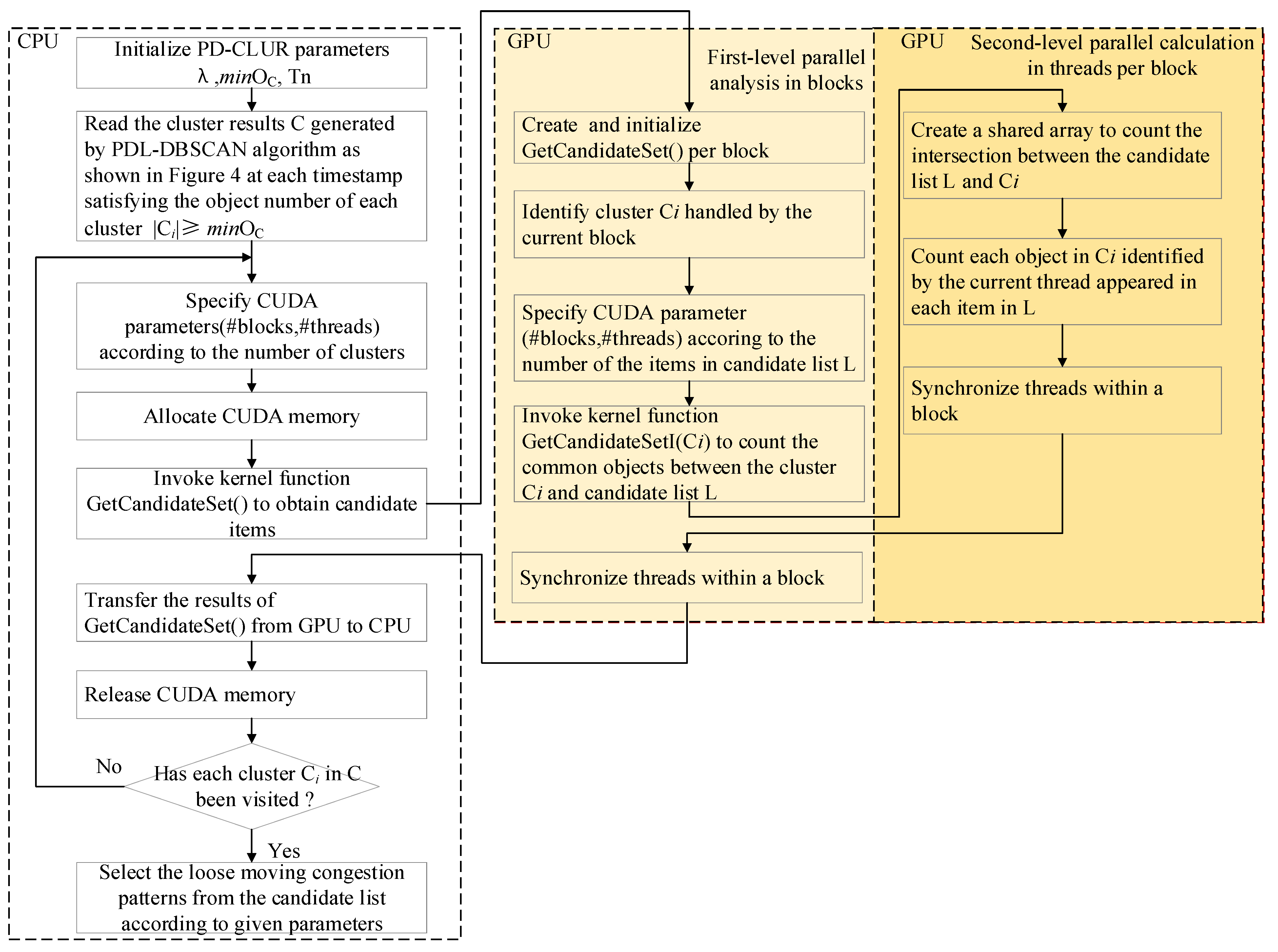
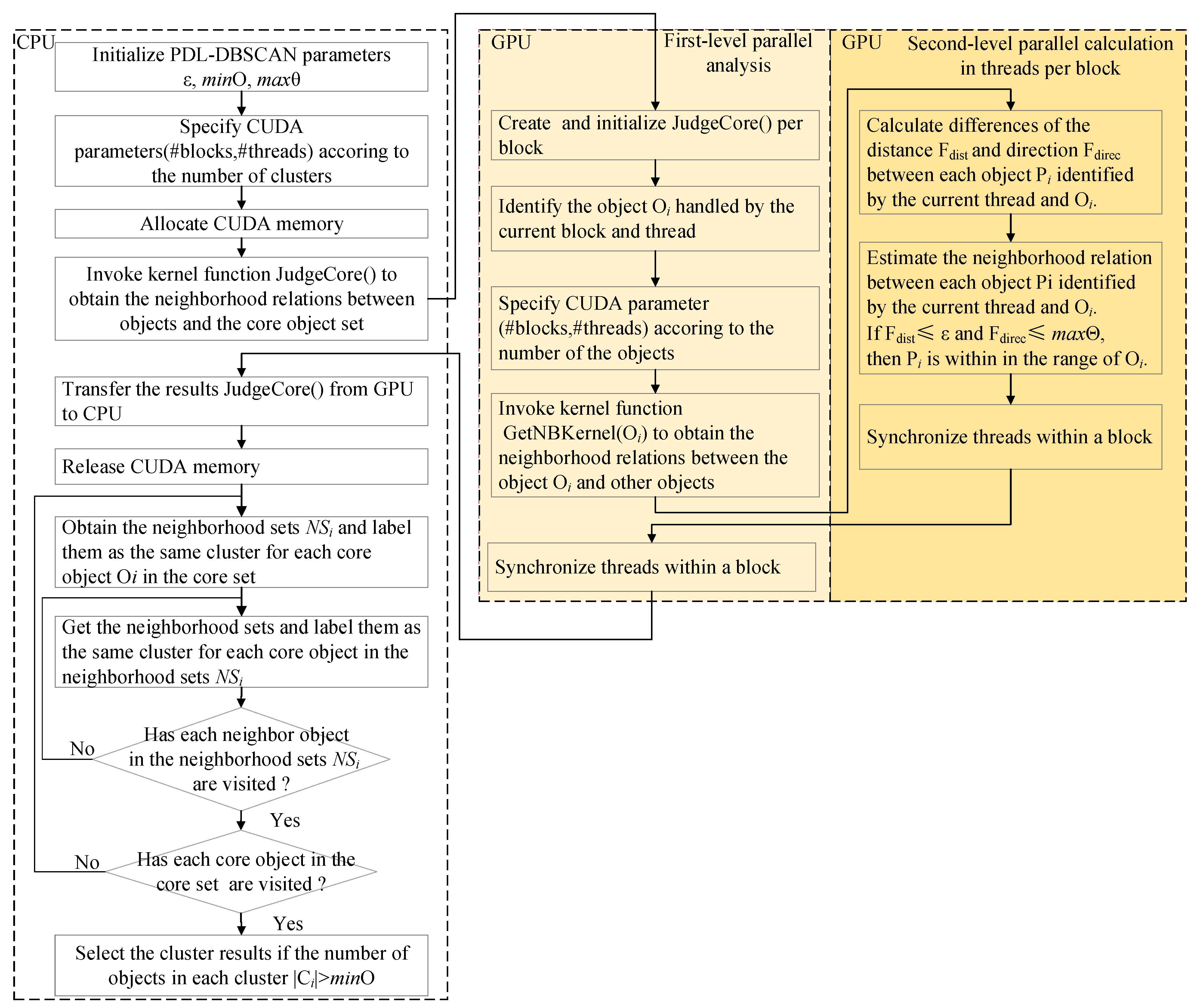
  • We propose an algorithm to discover loosely moving congestion patterns based on the characteristics of LMCP and the cluster-recombinant (CLUR) algorithm [10]. In order to achieve the high performance of the algorithm, we also designed a GPU-enabled parallel algorithm named PDCLUR based on the proposed discovery algorithm for handling the massive trajectory data.
  • We demonstrate the effectiveness and performance of the proposed algorithm as applied to an actual scenario. Compared with other group patterns like swarm, the discovery of LMCPs enables a better identification of congestion. Our results demonstrate certain significant congesting patterns pointing to the locations and timings of when the most congested patterns appear. Further, the proposed parallelized algorithm performs satisfactorily on handling large-scale datasets.
The rest of the paper is organized as follows. First, we review the related work on the spatiotemporal trajectory data analysis of moving objects. The next section illustrates the proposed concept and algorithm, with the penultimate section presenting our case study. Finally, we draw our conclusions in the final section.

2. Related Works

Related works on the spatiotemporal trajectory data analysis of moving objects essentially focus on three issues: (1) detecting traffic hotspots, (2) mining moving-object data, and (3) discovering group patterns. The conventional methods of hotspot detection include scan statistics [11] and kernel density estimation [12]. In addition to the above methods, the detection of hotspots by means of spatiotemporal data clustering methods including k-means and ordering points to identify the clustering structure (OPTICS) [13], DBSCAN [14], and grid-based clustering methods [15] has attracted intense research interest. In this context, Zhao et al. [16] proposed a trajectory clustering approach based on a decision graph and data field, which can select parameters for clustering, such as the number of clusters and cluster centers, to detect hotspots. The identified hotspots usually refer to geographical areas wherein the number of aggregates of objects exceeds an expected threshold. In this regard, a previous study [17] has introduced the trajectory box plot (TBP) to summarize and analyze trajectory streams, estimate their spatiotemporal density, and detect outliers. Obviously, the identification of dense traffic areas, which primarily exhibit crowding levels within a certain range instead of “regular” behavior, affords only static features rather than dynamic features. Meanwhile, other research works have focused on detecting spatiotemporal hotspots corresponding to urban resident behaviors [15], detecting networked and constrained hotspots of crimes [18], and so on.
The mining of moving-object data is an active research field. A moving cluster is defined as a sequence of spatial clusters, that is, clusters of moving objects gathered over consecutive snapshots [19]. Meanwhile, there are a large number of common objects appearing at consecutive time points during object movement [20]. In this regard, Wu et al. [21] proposed an automatic method to extract the profile of the regional representative moving modes of moving objects using trajectory data. The profile discovery of moving vehicles and animals can be used to detect road design flaws in urban planning and understand the habitual behaviors of animal migration under different geographical conditions, respectively. Unlike moving clusters, objects are “static” in spatiotemporal influence-based moving clusters proposed in the literature [22]. A spatiotemporal influence-based moving cluster refers to a sequence of spatial clusters that can exhibit the influence of their “spread” over a set of nearby objects; such clusters can be applied in the study of infectious diseases, ideas, etc. In a previous study [23], the authors proposed an approach to discover the dynamics patterns of leadership and followership by mining frequent patterns. In another study [24], the authors proposed a place-matching pattern-mining approach that enabled the identifying of stop episodes, refining stop-place candidates from OpenStreetMap (OSM), and subsequent matching using a hidden Markov model.
Here, we note that there is a growing interest in discovering group patterns of moving objects using trajectory data. The group patterns described by terms such as flocks [7], convoys [8], and swarms [9] refer to groups of objects moving together during a certain time periods. The flock patterns limit the range and shape of object clusters at each snapshot besides lasting for k consecutive timestamps. Different from the flock pattern, the shape of object clusters generated by the density-based spatial clustering of applications with noise (DBSCAN) algorithm is arbitrary for convoy patterns. While the swarm patterns may be employed in more application scenarios without the limitation of holding the pattern for k consecutive time points. The discovery algorithm of group patterns mostly searched the moving objects that satisfied the conditions of the pattern definition by building search space based on tree structure. The objectGrowth algorithm [9] used depth-first search strategy to find all subsets and checked if each subset is a swarm based on the object set search space. In order to reduce the search space, the authors proposed pruning strategies in the algorithm. Different from the objectGrowth algorithm, another algorithm CLUR [10] improved the algorithm performance by reducing the candidate item of the swarm based on defined inserting and updating rules. The inserting rules required that only the new candidate item which did not exist in previous candidate list be enabled to be inserted. While in the definition of updating rules, the key point checked if there is intersection between each candidate item needed to be updated and snapshot clusters. As regards group patterns, Zheng et al. [25] have pointed out that the abovementioned patterns are often unrealistic in practical group formations such as those in celebrations or parades. Therefore, they proposed gathering patterns that exhibit a dense and contiguous group of individuals without setting a coherent membership in the gathering. A gathering can be viewed as at least mp fixed objects appearing in kp clusters over a certain time period. This approach is more suitable for application to group events such as parades instead of traffic congestion pattern. In order to effectively and efficiently address a high volume of trajectory data, Zhang et al. [26] proposed a moving-object gathering pattern retrieval method based on spatio-temporal graphs. However, the performance of the retrieval method greatly depends on the construction of the spatiotemporal graph. Here, researchers noted that the interactions between moving objects would influence the mining of the group pattern as well as the dynamics. In a previous study [27], the concept of a crew was defined as a group of moving objects gathering with similar interactions and similar dynamics. The study also proposes a computational solution to discover crews from raw trajectory data. In this approach, the missing data points need to be filled for generating new fixes at the raw-data sampling rate because the movement parameters for interactions and dynamics are pairwise; this may limit the application of the approach. Zhao et al. [28] paid more attention to the converging pattern before moving objects gathered, and developed a mining framework. Furthermore, for improving the performance of online discovery of gathering patterns or converging pattern, various index structures like R-tree, quad-tree and grid have been introduced to accelerate computation [25,28]. Different from the discovery of group pattern, the related works in discovering traffic congestion mainly focused in traffic flow analysis [29], big data analysis [30] and so on. For instance, Kohan and Ale presented JamFlowScan algorithm [29] to discover the jam routes by finding hot routes based on speed and neighborhood searching for other jam routes based on the idea of DBSCAN. While in the literature [30], Zhao and Hu discovered the traffic congestion patterns from huge traffic monitoring information records by the congestion index analysis and K-mean clustering at the macro view. These studies rather differed from the discovery of group pattern and did not depend on moving object characteristics.

3. Methods

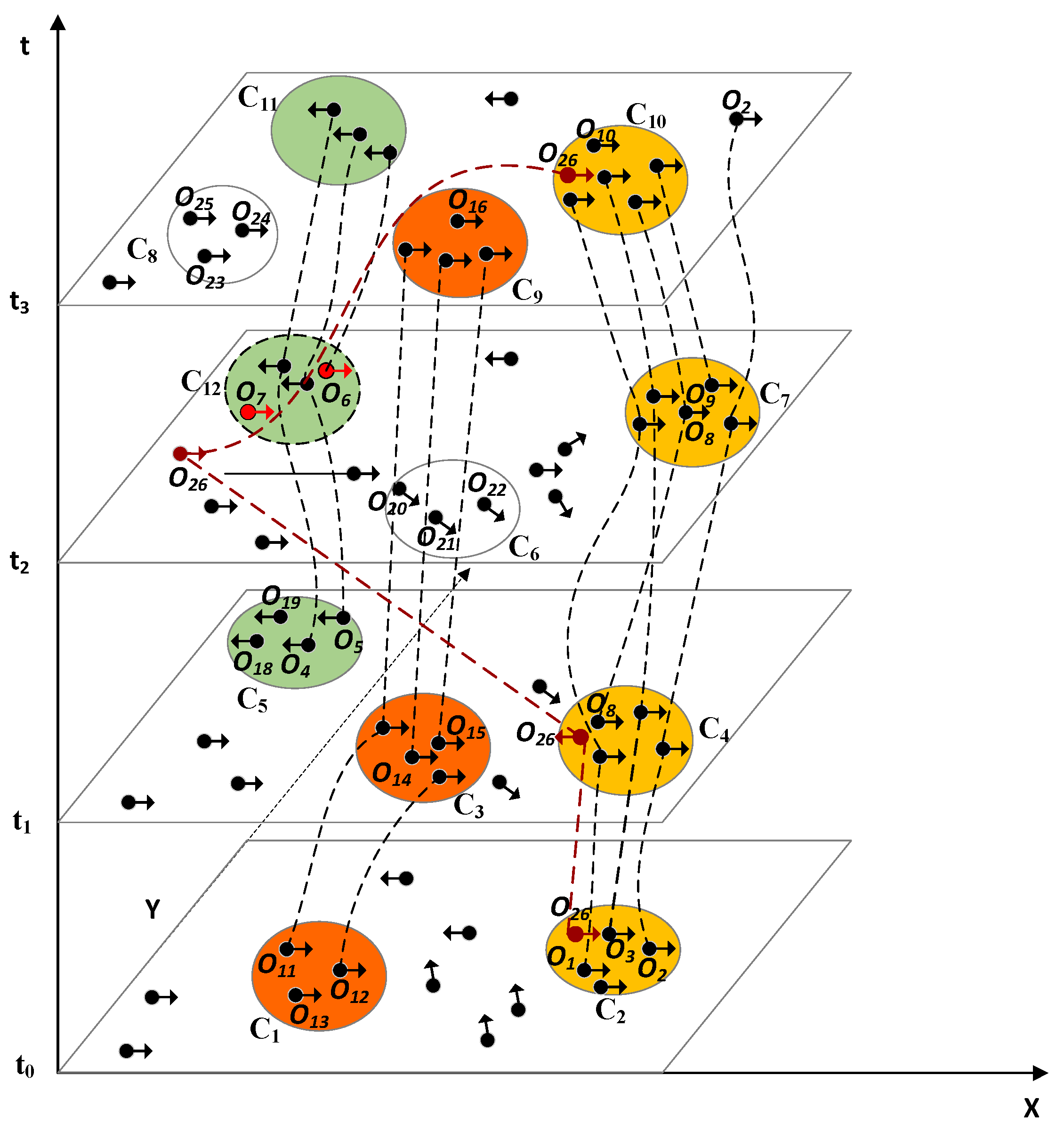
3.1. Concept and Definition

A loosely moving congestion pattern (LMCP) is a sequence of spatial clusters moving along a certain direction, wherein at least minOC objects holding an approximately similar moving direction gather in every cluster and at least λ common objects cluster together for at least two consecutive snapshots over the entire range of Tn time points. Essentially, a LMCP is expected to embody typical attributes of traffic congestion, such as high density, same moving direction, loose consistency moving feature, and duration. Among these features, high density refers to the concentration level of moving objects. In addition, the clustered objects can further exhibit a similar movement inclination. The loose consistency moving feature only requires that common objects travel together for at least two continuous time points instead of strict limitation on the continuity. The duration feature reflects the total time periods of congestion. The loosely moving congestion pattern can reveal traffic-congested roads instead of only near the junction or moving and crowded streams of individuals toward a certain target.
Let time period T = {t1, t2, …, ts} correspond to a series of time snapshots. Let O = {o1, o2,…,om} be a collection of objects that have moved toward a certain direction during time period T.
Definition 1.
A non-empty set of objects Ctij     O can be defined as an equidirectional spatial snapshot cluster at time point ti when each object in this spatial cluster moves along approximately the same direction and is densely connected to other objects in terms of the spatial distribution. We note here that there may be several equidirectional spatial snapshot clusters {Cti1, Cti2, …, Ctir} (r ≤ m) at time point ti.
Definition 2.
A loosely moving congestion pattern (LMCP) is expressed as <C, Tn, D>, where C = {Ctij, Cti+1k, …, Cti+n q} (1 ≤ j ≤ r, 1 ≤ k ≤ r, 1 ≤ q ≤ r) denotes a sequence of equidirectional spatial snapshot clusters moving along approximately the same direction D lasting Tn time points during time period T, such that
  • each Ctij C represents an equidirectional spatial snapshot cluster at timestamp ti for each i (1 ≤ i < s),
  • spatial cluster Cti+1k at timestamp ti+1 is formed after Ctij at timestamp ti for each i (1 ≤ i < s),
  • there are at least two equidirectional spatial snapshot clusters Ctij and Cti+1k in C satisfying |Cti j ∩ Cti+1k | ≥ λ (the common object number between two consecutive equidirectional spatial snapshot clusters), where λ denotes an integer >2 during T,
  • there are totally Tn time points satisfying |Ctij| ≥ minOC for each i (1 ≤ i < s) during time period T, where minOC denotes an integer >2 during T, and
  • all equidirectional spatial snapshot clusters exhibit approximately the same moving direction D in a LMCP.
The LMCP is rather different from previous group patterns like a swarm. A pair (O, T) is defined as a swarm if it satisfies three requirements [9]: (1) the objects number in the set O should be at least mino; (2) the objects in O are in the same cluster for at least mint; (3) there is at least one cluster containing all the objects in O at each time point. We illustrate Definition 2 and differences between LMCP and swarm using an example given in Figure 1. We observe that there is a cluster sequence {C2, C4, C7, C10} in Figure 1 when we set λ = 3, minOC = 3, and Tn = 4. Let λ = 2, minOC = 3, and Tn = 3, and consequently, the two sequences {C2, C4, C7, C10} and {C1, C3, C9} represent all cluster sequences of the LMCP in which each snapshot cluster contains at least two common objects holding at least two consecutive time points along the same movement direction during the given time periods. For the parameters setting, the smaller the value of the parameters λ, minOC and Tn, the more LMCPs we obtain. Meanwhile, new members can constantly “enter” each snapshot spatial cluster, such as objects O8 and O9 entering the equidirectional spatial snapshot clusters C4 and C7, respectively. Of course, there are also members, such as object O2 that has “exited” the snapshot spatial cluster C10 at timestamp t3. The set {C5, C12, C11} is not a cluster sequence of LMCP because C12 is not an equidirectional spatial snapshot cluster in which the moving directions of objects O6 and O7 are not consistent with the moving directions of other objects O4, O5 in cluster C12. In our algorithm, the two objects O6 and O7 cannot be gathered in cluster C12. If we set the thresholds of the swarm mino = 2 and mint = 3, there are three swarms: ({O1,O2,O3},{t0,t1,t2}), ({O1,O3,O8},{t1,t2,t3}) and ({O1,O3,O26}, {t0,t1,t3}). From Figure 1, we find that the swarm ({O1,O3,O26}, {t0,t1,t3}) contains the object O26 although its trajectory deviate others at timestamp t2. While in LMCP, the object O26 is not included in the cluster C4. If we set λ = 3, minOC = 5, and Tn = 3, there is only one snapshot cluster sequence {C2, C7, C10} in LMCP.

3.2. Pattern Discovery Algorithm

This paper mainly focuses on efficiently discovering LMCPs based on the CLUR algorithm [10], which was employed discovering the swarms. In order to extract the LMCPs, we develop three rules for creating new candidate items, updating the candidate list at each timestamp and identifying LMCPs finally. Given a spatial clusters Cti = {Cti1, Cti2, …, Ctin} at timestamp ti, which these clusters can be obtained by spatial clustering, we consider the following rules:
Rule 1.
For any spatial snapshot cluster Ctij at time point ti (1 ≤ j ≤ n), if the number of moving objects within it |Ctij| ≥ minOC and |Omd − Ond| ≤ maxθ (Omd and Ond belong to the range of the approximate direction D) for   Om∈Ctij and   On∈ Ctij (1 ≤ j ≤ n), where Omd and Ond denote the movement directions of Om and On, respectively, then Ctij is an equidirectional spatial snapshot cluster at timestamp ti, and a new candidate item <Ctij, ti, D > (D denotes the directional value) is created in the candidate list L of LMCPs.
Rule 2.
For any candidate item V = < Ctij, T, D> ∈ L (1 ≤ j ≤ n), if Cti+1k is an equidirectional spatial snapshot cluster at timestamp ti+1 and| Ctij ∩ Cti+1k | ≥ λ (there are λ common objects for two equidirectional spatial snapshot clusters Ctij and ti+1k), |Omd − Ond| ≤ maxθ for Om ∈ Ctij and   On ∈ Cti+1k (1 ≤ k ≤ n), then V is updated as <{Ctij, Cti+1k}, T ∪ {ti+1},D> in the candidate list L.
Rule 3.
For any candidate item V = <C, T, D> ∈ L (C = { Ctij, Cti+1k,…, Cti+nl}), if |T| ≥ Tn (Tn ≥ 2 represents the total lasting time) satisfying the condition: i : 1 i < i + 1 < n , t i T t i + 1 T = t r u e , then <C, T, D> is a loosely moving congestion pattern (LMCP).
Rule 1 is employed to create a new candidate item of LMCP at time point ti which is expressed as a triple < Ctij, ti, D>. We need to estimate whether or not a cluster Ctij is an equidirectional spatial snapshot cluster according to two conditions: (1) the number of objects within the cluster is greater than a given threshold minOC; (2) the difference of the direction value between objects within the same cluster is less than a given threshold maxθ. While rule 2 give the conditions of updating candidate item, one is the common object number of two consecutive snapshot cluster Ctk and Cti+1k, the other is the difference of the direction value between objects respectively within two consecutive snapshot cluster Ctk and Cti+1k. The rule can ensure that there are λ objects moving together toward the approximate same direction. Finally, a LMCP is identified from candidate list L when the total time points of a candidate item are greater than a given threshold Tn and a candidate item keeps at least two consecutive times points according to rule 3.
Based on these rules, we propose an algorithm for discovering LMCPs. This algorithm firstly performs spatial clustering of moving objects via the DBSCAN algorithm adding direction limitation at each timestamp. Next, we build and update a list of candidate items according to rules 1 and 2 at each timestamp. Finally, the LMCPs are identified according to rule 3. As an example, the discovery process of moving congestion patterns in Figure 1 is captured in Table 1. Before the generation of the candidate items, the equidirectional spatial snapshot clusters from C1 to C11 are obtained by the DBSCAN algorithm adding direction limitation. At the first timestamp t0, there are two candidate items V1 = <C2, t0, 0> and V2 = <C1, t0, 0> that satisfy the condition |C| ≥ minOC (minOC = 3), with the same moving directions of all objects within same cluster according to rule 1. Next, at timestamp t1, the candidate items V1 and V2 are, respectively, updated as <{C2, C4}, {t0, t1},0> and <{C1, C3}, {t0, t1},0> according to rules 2 when the parameter λ = 2. At the same time, the candidate item V3 = <C5, t1, π> is created at timestamp t1 according to rule 1. At time point t2, the moving directions of the objects within the cluster C12 are not consistent, and therefore, the cluster C12 is not created (minOC = 3) as per our modified DBSCAN algorithm. The candidate item <C12, t2, π>, indicated in italics, is not included in the candidate list. At the last timestamp t3, only two candidate items, <{C2, C4, C7, C10}, {t0, t1, t2, t3},0> and <{C1, C3, C9}, {t1, t2, t3},0>, correspond to the definition of LMCP according to rule 3 when we set Tn = 3 and λ = 2. In particular, an item <{C5, C12, C11}, {t1, t2, t3},π> is not a LMCP, as mentioned above. Furthermore, if we neglect cluster C12, the item <{C5, C11}, {t1, t3},π> cannot satisfy the condition holding at least two consecutive time points during the moving process as per rule 3.
Algorithm 1 presents the pseudo-code for discovering LMCPs. Given the input parameters like the candidate list L, snapshot clusters set Clusters, threshold minOC, maxθ,Tn and λ, the possible LMCPs will be generated by creating and updating candidate items. At each time point, we check each cluster of current snapshot clusters to see if it can become a candidate item. If so, the new candidate item will be created and inserted into next list as shown in lines 7–11 in Algorithm 1. Then we check each candidate item in candidate list L to see if it can be updated according to rule 2. The Lines 12–20 outlines the process. Meanwhile, we also insert the updated item into the next list. At last, all candidate items which satisfy the conditions of pattern identification will be inserted into the LMCPs list.
Algorithm 1. Discovering LMCPs
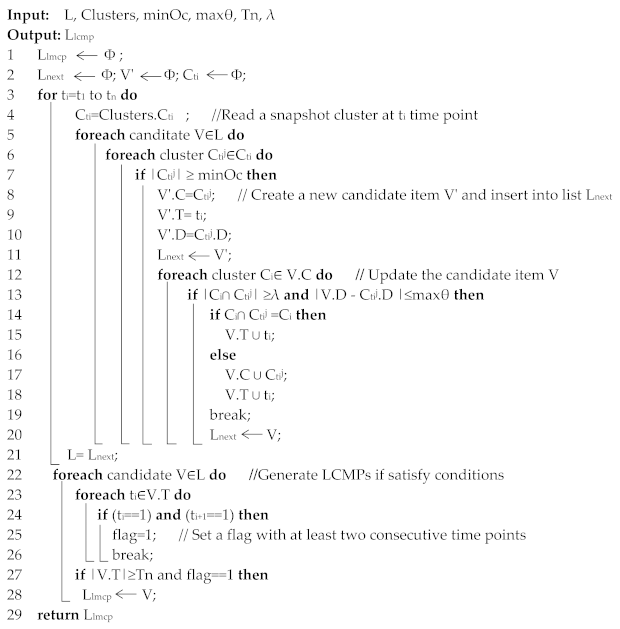
Ijgi 10 00787 i001
In order to accelerate the pattern discovery, we designed a GPU-enabled parallel algorithm named PDCLUR based on Algorithm 1 using Compute Unified Device Architecture (CUDA) (Figure 2). PDCLUR initializes the parameters and reads the clustering results generated by parallel computing adding direction limitation on DBSCAN (PDL-DBSCAN) algorithm, as shown in the flow chart in Figure 3, at each timestamp within the CPU environments, and then switches to the memory of GPU after specifying the CUDA parameters and allocating the CUDA memory for advanced calculations. The kernel function GetCandidateSet is employed to parallelize the discovery of LMCP. In this algorithm, two-level parallel computing is carried out, wherein all clusters at each timestamp are addressed as blocks within the global memory of the GPU environments via first-level parallel computing. Moreover, the calculations of the intersection between each cluster at each timestamp and each item in candidate list L are performed on a large number of threads invoked by kernel function GetCandidateSetI for implementing second-level parallel computing.
The PDL-DBSCAN algorithm also utilizes two-level parallelized computing by means of the kernel functions JudgeCore and GetNBKernel to obtain the core object set and the neighborhood relation between any two objects, respectively, which is a primary step for generating the neighborhood of each core object (this computation greatly affects the algorithm efficiency) using CUDA, as shown in Figure 3. An important point to estimate the neighborhood relation in the kernel function GetNBKernel takes account of not only the distance difference but also direction difference between objects. In PDCLUR and PDL-DBSCAN, the choice of the appropriate CUDA parameters (blocks and threads) for the parallel kernel function is dependent on the GPU device used. For example, each GPU device (GeForce RTX 2080) used in this study has up to 65,535 × 1024 threads.

4. Case Study

In order to evaluate the efficiency and effectiveness of the discovery algorithm of LMCPs, a comprehensive performance study has been conducted on two trajectory datasets with different size. The first dataset [31] contains 664 electric taxi GPS samples for one day on 22 October 2014 in the city Shenzhen including vehicle id, longitude, latitude, time, speed. We sampled 61,683 trajectory points from the dataset at a 1-min interval from 5 to 6 pm. These sampled trajectory points would be used to implement the experiment for the discovery of LMCPs. Because the data volume is small, we only used the Algorithm 1 to conduct the pattern discovery instead of parallel algorithm. The second dataset contains approximately 33,900,000 trajectory points generated by nearly 14,000 taxis in Beijing in November 2012. Trajectory points within 24-h per day were collected at about 1-min time interval, and each trajectory point contained the taxi’s trajectory information such as geographic position, speed, direction, timestamp and so on. In our study, a large number of taxi trajectory points were extracted during the morning (7–9 a.m.) and evening peak (5–7 p.m.) times for discovering LMCPs. The data of nearly 7900 taxis were extracted to calculation after data preprocessing, which included the removal of noisy data and sampling according to time granularity (5 min), during the daily morning peak traffic period. Similarly, the data of approximately 8800 taxis were extracted to pattern analysis during the daily evening peak time. For the second dataset, we implemented the PDCLUR algorithm to discover LMCPs. Through the case study, we expected to obtain valuable traffic information including the most congested road segments, congestion time, congestion directions and so on.

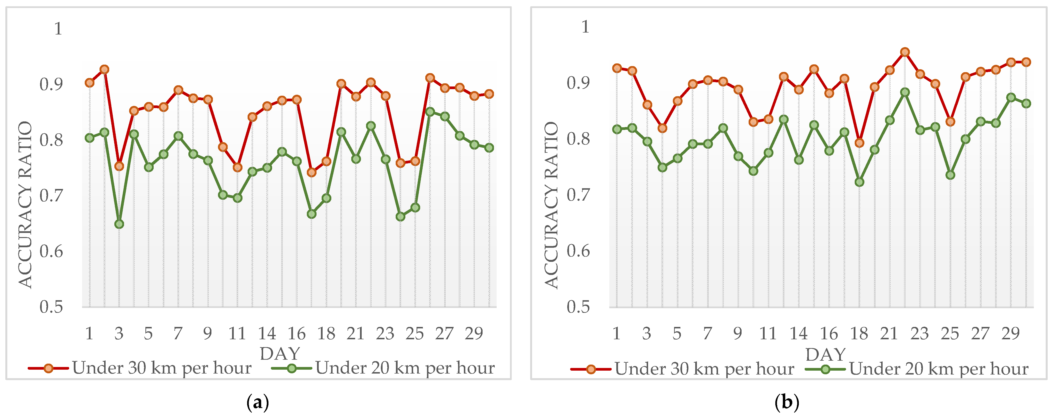
4.1. Algorithm Effectiveness Analysis and Discussion

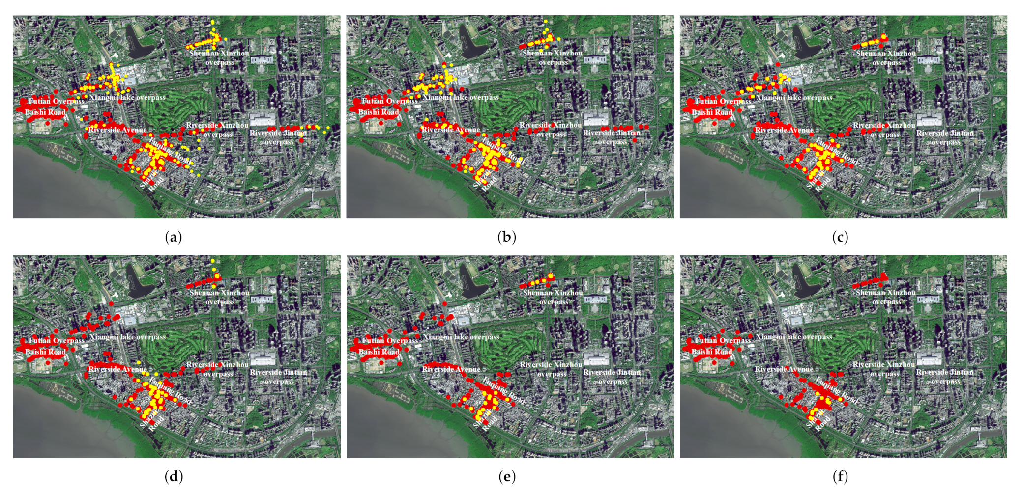
4.1.1. Effectiveness of LMCP Discovery Algorithm for Shenzhen Samples Dataset

In this case study, we used a total of 60 timestamps data from 5 to 6 pm according to 1-min interval. Next, we traced the trajectory point of every taxi at every time snapshot. The dataset lacks the direction information of each trajectory point. Thus, the default parameters used in this dataset of experiments are minOc = 5, Tn = 3 and λ. The parameter λ denotes the number of common objects between two consecutive snapshot cluster and is key for the discovery of LMCPs. We compared experimental results caused by setting different parameter λ. Meanwhile, we also compared the discovered LMCP with the swarm when the parameters λ and mino (at least the objects number in the object set O of swarm) were respectively set to different values. By setting λ = 3 to 8, we found 86, 84, 82, 76, 70 and 65 LMCPs, respectively. While setting mino = 3 to 5, the swarms we found were all 32. When we set mino = 6 to 8, there were 22, 16 and 16 swarms, respectively. Obviously, the discovery algorithm of LMCP can generate more group patterns.
The main experimental results are shown in Figure 4. The red trajectory points plotted in the Shenzhen image denoted the LMCPs generated by Algorithm 1, while the yellow trajectory points denoted the swarms generated by CLUR. Our algorithm can find the main four congested road segments like Futian Overpass, Baishi Road, Fuqiang Road and Shenan Xiuzhou Overpass in all settings of the parameter λ. To evaluate the validity of the discovery of LMCPs, we used the congestion index like speed to verify the results. By the calculations on the trajectory points belonging to LMCPs from 5 to 6 pm, the average speeds of the identified road segments were all at low speed, respectively 20, 18, 9 and 10 km per hour. In Figure 4a,b, we find that the key differences between two patterns focus on five road segments in the LMCPs: Futian Overpass, Baishi Road, Riverside Avenue, Riverside Xinzhou Overpass and Riverside Jintian Overpass. Correspondingly, the average speeds of these roads were, respectively, 20, 18, 10,16 and 13 km per hour. In Figure 4c, three congested segments, like Futian Overpass, Baishi road and Riverside Avenue, were discovered by our algorithm instead of CLUR. In Figure 4d–f, yellow trajectory points became less and less with the parameter mino increased. In particular, the discovery of swarm has hardly detected the congested road segments in Figure 4f. These findings indicated that our discovery of LMCPs outperforms the swarms for detecting the congestion pattern.

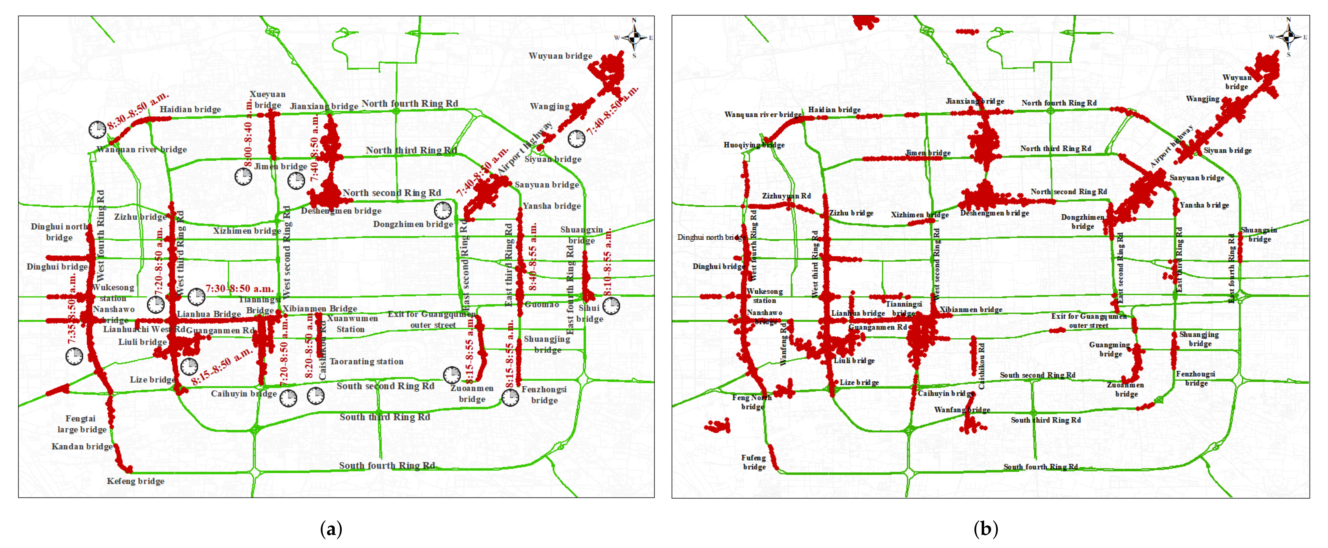
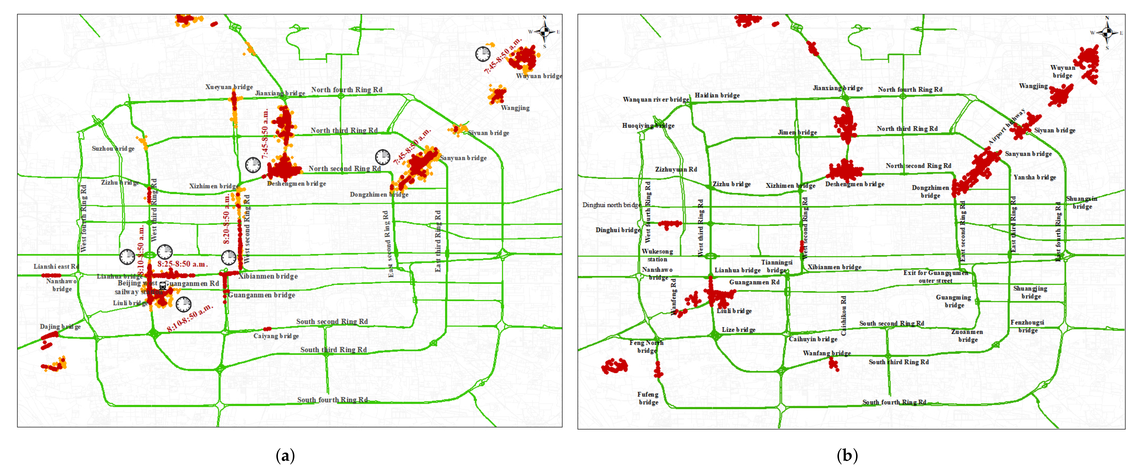
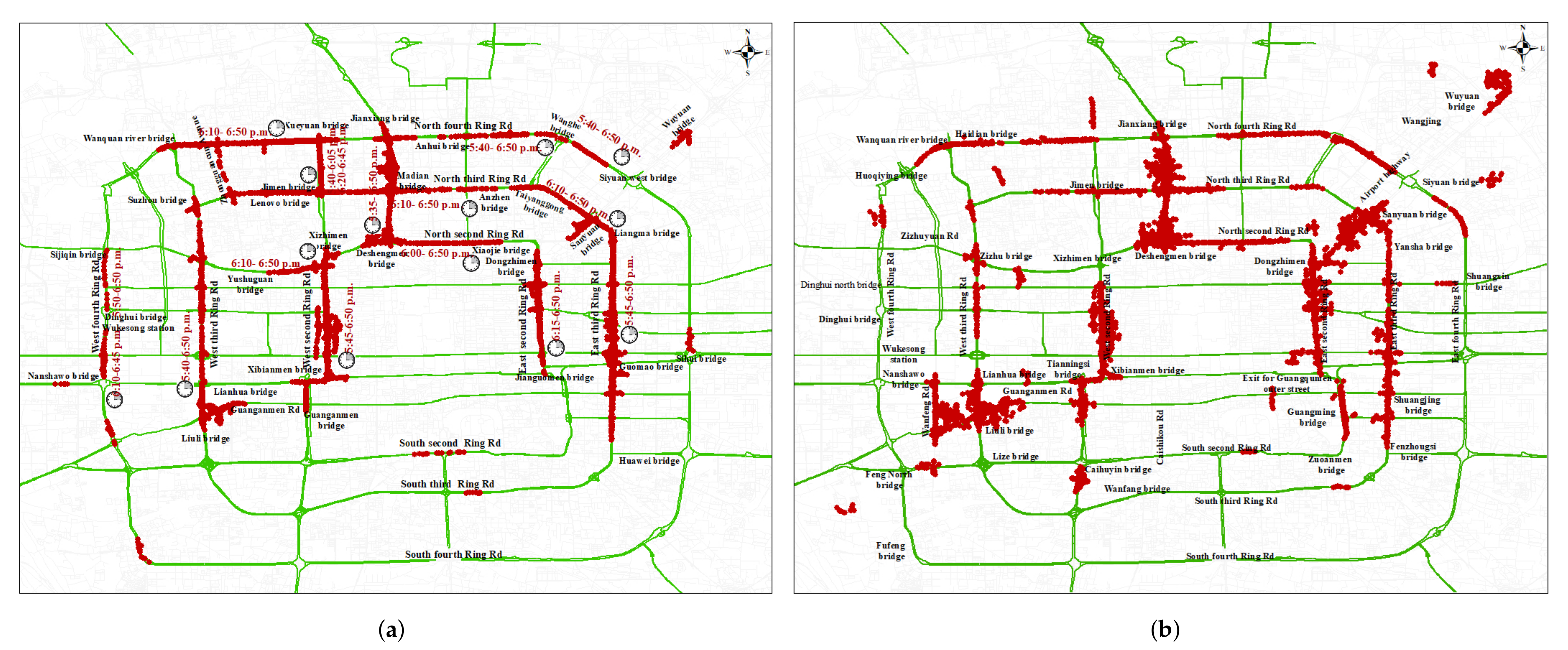
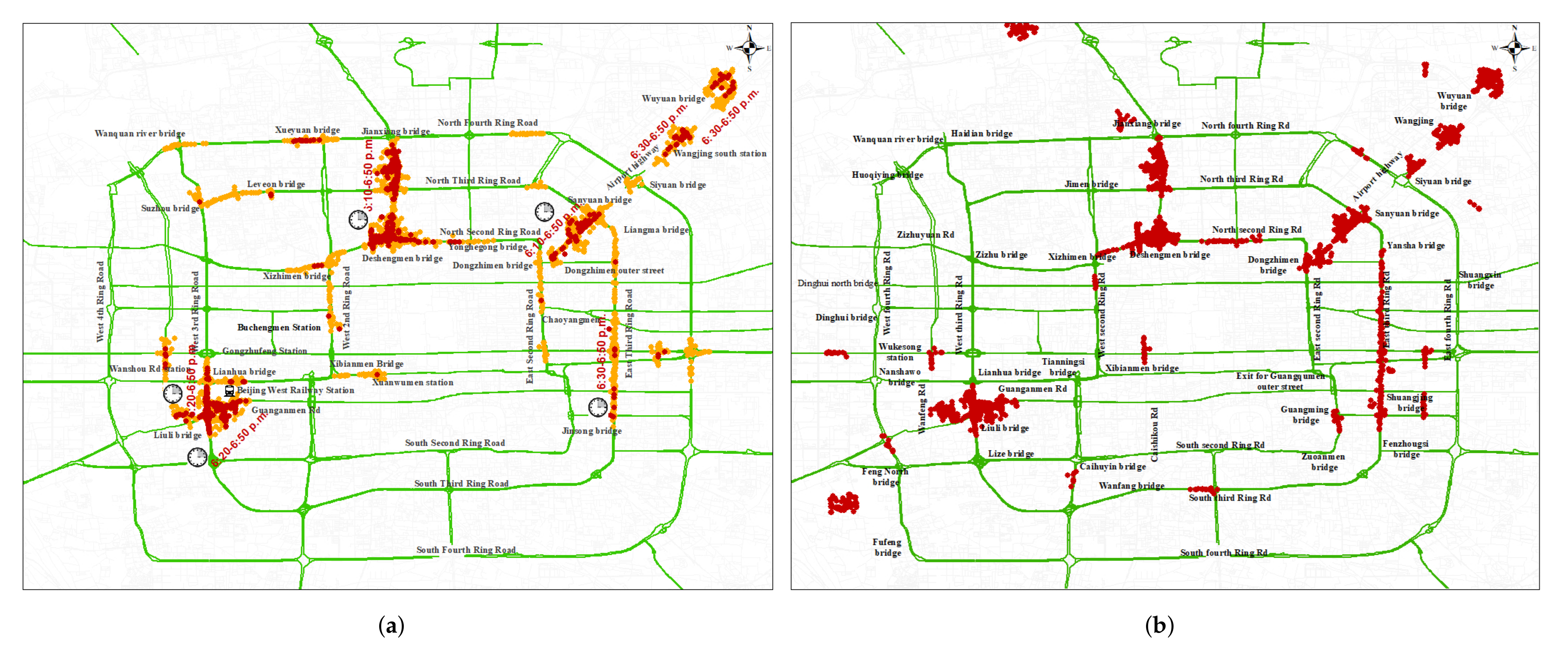
4.1.2. Effectiveness of LMCP Discovery Algorithm for Beijing Samples Dataset

In the second case study, CUDA version 9.1 was chosen to implement our GPU-based PDCLUR algorithm. The programming language used was C/C++, and the operating system was Windows. The GPU device used in this study was the NVIDIA GeForce RTX 2080 (2944 CUDA cores, 1.8 GHz clock rate, 8 GB global memory, and 64 computing units of peak performance for double-precision floating point operations). The CPU used for sequential computing was the Intel Core i7 6700 (dual four-core processor) with 3.4 GHz clock frequency and 16 GB memory.
We firstly discretized the peak time (7–9 a.m. and 5–7 p.m.) into different time points according to 5-min intervals. Thus, there are a total of 24 timestamps during the morning and evening peak intervals. Next, we traced the trajectory point of every taxi at every time snapshot. We set the algorithm parameters as minOc = 8, λ = 5, Tn = 3, maxθ = 0.4 (in radians). That is to say, no less than eight taxis are required to move together at every time point, of which at least five taxis keep moving together for 10 min. In addition, no less than five taxis in two snapshot clusters, which are not always continuous, merge together during no less than 15 min. For obtaining the snapshot clusters at each time point, we applied the PDL-DBSCAN algorithm with CUDA and settings of minO = 8, ε = 300 (m).
The effectiveness of our algorithm was evaluated via discovering LMCPs, using which we could determine the most congested road segments, time periods of the congestions, and congested differences between weekday and weekend morning peak (7–9 a.m.) and evening (5–7 p.m.) hours. In order to verify the validity of our algorithm, furthermore, we compared the discovered LMCPs with the generated swarm pattern by CLUR algorithm.
In the study, we found that in Beijing city, during the morning peak hours on working days from Monday to Friday (Figure 5a), the congested roads (rendered in red color) were mainly the West second Ring Road, West third Ring Road, West fourth Ring Road, North fourth Ring Road, area around Wangjing, and East third Ring Road. In addition, according to the direction of equidirectional spatial snapshot clusters in LCMPs, we found that the direction of traffic jams was chiefly aligned from the south to north in Beijing city. Among these congested roads, the segment from Caihuyin bridge to Tianningsi bridge in the West second Ring Road was severely congested. The most congested segment of the West third Ring Road spanned from Lize bridge to Zizhu bridge. Meanwhile, on the West fourth Ring Road, traffic jams occurred at two road segments: from Kefeng bridge to Kandan bridge and from Fengtai large bridge to Dinghui north bridge. On the West fourth Ring Road, there was a certain degree of congestion around Nanshawo bridge, Wukesong, and Dinghui bridge. Moreover, in the east region of the city, traffic jams occurred on East second Ring Road, East third Ring Road, and East fourth Ring Road. In particular, we determined two congested road segments from Fenzhongsi bridge to Shuangjing bridge and from Guomao station to Yansha bridge on the East third Ring Road. Serious congestions emerged in certain segments of the airport highway from Dongzhimen to Sanyuan bridge and from Siyuan bridge to Wuyuan bridge. In the north of the city, the road segment from Wanquan river bridge to Haidian bridge was congested on the North fourth Ring Road. Traffic on the road from Deshengmen bridge to Jianxiang bridge connecting North second Ring Road to North fourth Ring Road was heavy. In addition, the road section from Jimen bridge to Xueyuan bridge parallel to this road was also congested. From the west to east, severe congestion was observed from Lianhuachi west road to Xibianmen bridge. The time period of the congestion period mainly ranged from 7:20 to 8:55 a.m. Compared to the swarm pattern generated by CLUR algorithm (Figure 4b), the LMCPs almost embodied all the swarm pattern besides one section of Zizhuyuan road on North second Ring Road and another section around Jimen bridge on North third Ring Road. Our algorithm discovered more congested roads like the section from Guomao station to Yansha bridge on the East third Ring Road. To compare the results between LMCPs and swarm, we analyzed the actual road situation by evaluating the congestion index like speed. We calculated the average speed per day for all taxis belonging to the LMCPs on the East third Ring Road. For each working day, there may be 3 or 4 days of taxi data belonging to LMCPs in a month. Thus, we calculate at most three days of data belonging LMCPs per working day. In Figure 6a, we use four values to present the congestion level for each working day. The first three values are the taxis’ average speeds of three days belonging to the LMCPs on each working day, and the fourth value represents the average value of three days to show the overall average level. There was only one day of data on Monday, Tuesday and Friday. According to the local standard “Urban Road Traffic Operation Evaluation Index System” in Beijing city, the speed on the main road is mild congestion at 20 to 30 km per hour, moderate congestion at 15 to 20 km per hour, and heavy congestion below 15 km per hour. From the Figure 6a, we can see that all values are below 30 km per hour, and all average values per working day are below 20 km per hour. That means the road was congested, and our result like the congested road on East third Ring Road was consistent with the actual road situation during morning peak hours on working days.
Relative to weekdays, weekend traffic jams (Figure 7a) were greatly reduced from 7:00 to 9:00 a.m. Congestion was mainly concentrated at four road sections: from Guanganmen bridge to Xizhimen bridge on West second Ring Road, from Liuli bridge to Lianhua bridge near the Beijing west railway station on West third Ring Road, from Deshengmen bridge to Jianxiang bridge on the road connecting North second Ring Road and North fourth Central Road, and from Dongzhimen bridge to Sanyuan bridge and near Siyuan bridge, Wangjing, and Wuyuan bridge in the direction of the airport highway. In addition, traffic jams were also observed in the road section from Lianhua bridge to Xibianmen bridge in the west–east direction. The time interval of this congestion period mainly ranged from 7:45 to 8:50 a.m. Compared with the swarm pattern shown in Figure 6b, our algorithm generated more results like the congested road from Guanganmen bridge to Xizhimen bridge on West second Ring Road and other congested road between Lianhua bridge and Xibianmen bridge.
As shown in Figure 8a, during the evening peak traffic hours, congestion primarily appeared on the East third Ring Road, East second Ring Road, West second Ring Road, West third Ring Road, and the road segment from Deshengmen bridge to Jianxiang bridge that connects North second Ring Road to North fourth Ring Road from the south to the north. In addition, congestion was observed in the segment from Jimen bridge to Xueyuan bridge from south to north. From east to west, there were two congested roads on the North fourth Ring Road: from Wanhe bridge to Anhui bridge and from Xueyuan bridge to Wanquan river bridge. On the North third Ring Road, traffic jams spanned a long distance from Anzhen bridge to Zhongguancun avenue crossing. On the North second Ring Road, congestion ranged from Xiaojie bridge to Deshengmen bridge. From east to north, traffic was heavy in two road sections from Liangma bridge on the East third Ring Road to Taiyanggong bridge on the North third Ring Road and from Siyuan West bridge to Wanghe bridge on the North fourth Ring Road. From the generated results by the CLUR algorithm shown in Figure 8b, we can see that heavy traffic congestion also appeared on the same roads, basically. The main difference between LMCPs and swarm pattern was the congested road from Nanshawo bridge to Sijiqin bridge on West fourth Ring Road by our algorithm and the road on Wanfeng road by the CLUR algorithm. As before, we also compared the results between LMCPs and swarm by evaluating the congestion index. As shown in Figure 6b, all values are below 30 km per hour, and all average values per working day are below 20 km per hour on the road from Nanshawo bridge to Sijiqin bridge on West fourth Ring Road during evening peak traffic hour. This means that our results are more consistent with the actual road situation compared to the swarms. Meanwhile, our results also show that the congestion period is mainly concentrated between 5:30 and 6:50 p.m. These results are also consistent with the actual traffic situation. Basically, most workplaces are normally closed by 5:00 p.m. in Beijing, which corresponds to the beginning of the evening rush hour. We hypothesize that it takes about 30 min for a large number of vehicles to enter the road segments, which results in traffic congestion. Traffic significantly reduces after 6:50 p.m., thereby signaling the end of the evening peak.
Traffic on Saturdays and Sundays was slight between 5:00 and 7:00 p.m., which is the time interval corresponding to the evening peak situation on working days. From the discovered congested pattern by our algorithm and the CLUR algorithm shown in Figure 9, congestions were mainly observed on roads near the Beijing west railway station, airport highway, and the central road connecting the North second Ring Road to the North fourth Ring Road. For LMCPS, traffic jams were mainly observed after 6 p.m. In addition to these congested roads, slight congestions appeared on the East third Ring Road and East second Ring Road, near Xueyuan bridge on the North fourth Ring Road, Suzhou bridge on the North third Ring Road, and Xizhimen bridge on the West second Ring Road.
From the discovery of congestion patterns, we have reason to believe that the number of traffic lights and junctions are a possible because of traffic congestion. For instance, traffic congestion on the road from Deshengmen bridge to Jianxiang bridge connecting North second Ring Road to North fourth Ring Road was heavy whether travel time was morning or evening peak hours, working day or weekend. Obviously, there are more junctions on the congested road than other road from geographic location and road network structure. On the other hand, the traffic pressure on the second and third ring roads is great as a result of road network structure lacking of fast link lines between these ring roads. From our results of the discovery of congestion patterns, traffic jam usually was heavy on the second and third ring roads in east, west and north of the city. Other possible causes of traffic congestion include the division of urban functional zones, road capacity and so on.
We also report the evaluated results of LMCPs using the congestion index like speed. Figure 10a,b respectively present the accuracy ratios of the discovery of LMCPs during morning and evening peak traffic hours within 30 days. The red line represents the ratio of the number of taxis per day belonging to LMCPs, which their speeds were under 30 km per hour (mild congestion), to all number of taxis per day belonging to LMCPs. While the green line represents the ratio under 20 km per hour (moderate congestion). The accuracy ratios under 30 km per hour are higher than those under 20 km per hour. In Figure 10a, the lower values occur on November 3, 11, 17, 24 and 25 whatever under 30 km per hour or under 20 km per hour. Besides these days, other values are closed to 0.9 or above 0.9 when the speed of taxis, belonging to LMCPs, was under 30 km per hour. While under 20 km per hour, the accuracy ratios are closed to 0.8 or above 0.8. Similarly, the lower values emerge on 4 November, 10,18 and 25 in Figure 10b. The lower accuracy ratios all occur on weekend. The reason is that traffic jam on weekend is not heavy compared with weekdays. As a whole, the accuracy ratio during evening peak traffic hours are higher than those during morning peak traffic hours. From the evaluation results of the discovery of LMCPs, our approach presents benefic effectiveness in identifying the congestion pattern.

4.2. Algorithm Performance

This section focuses on the evaluation of the performance of our GPU-based parallel computing algorithm. Here, we note that the number of trajectory points and the choice of GPU are the primary factors that affect the acceleration performance of the algorithm. In the study, we compared the running times of pattern discovery between GPU-based parallel computing and CPU-based sequential computing. We tested >4,300,000 points and >5,400,000 points over 28 days during the morning and evening peak hours, respectively.
As discussed previously, our algorithm consists of two complicated calculation processes: clustering and searching candidate items. In our algorithm, the core calculation with high computation complexity is executed by means of parallel computing. Thus, the computing environment includes a CPU as well as the GPU. In our study, we applied the DBSCAN algorithm by appending a direction limitation within the same cluster and using CUDA. For nearly 170,000 points over 24 h, including the data of 24 times snapshots during the morning peak time, an average of ~7900 points in each time snapshot is clustered. In addition, the threads of the first-level and second-level parallel calculations in the PDL-DBSCAN algorithm are all set to 16 × 512. In contrast, the number of each time snapshot of one day during the evening peak interval was approximately 8800 points, which means that the threads of parallel calculation also increase to 18 × 512. For searching the candidate items of LMCPs for one day, we conducted four calculation traverses considering the limitation of the CUDA computing environment; the number of blocks was set to 100 during the first-level parallel analysis and the number of threads was set to 128 × 100 during the second-level parallel calculation for each traverse.
Table 2 and Table 3, respectively, present the computing performance results during the morning and evening peak intervals from day 1 to day 28. From Table 2, we note that the running time, both sequential Algorithm 1 and PDCLUR with parallel computing, increases as the number of trajectory points increases. However, our algorithm, using parallel computing, can significantly enhance the computing performance. For example, the sequential calculation time for discovering the LMCPs of one day using the Algorithm 1 is 950 s during the morning peak time. On the other hand, upon applying PDCLUR with GPU acceleration, only 13 s are needed to discover the loose moving congestion patterns of one day during the morning peak time. For ~4.34 million points across 28 days, the sequential calculation time amounts to 24,056 s. On the other hand, the total computing time using GPU for pattern discovery is only 352 s when the GPU with 64 computing units is used to handle the 28-day data. Here, we use the ratio of the running time of the PDCLUR algorithm involving parallel and sequential computing to the execution time of the sequential computing of the algorithm using only the CPU to evaluate the computing performance. Although the acceleration ratio slightly decreases as the number of points increases, we find that the acceleration ratio is generally very high (>65, Table 2 and Table 3). Here, we also note that the data transfer rate between the CPU and GPU increases as the number of points increases; this factor can thus affect the acceleration performance. However, the frequency of data transfer reduces with increase in the number of GPUs working together or when the computing performance of the single GPU is upgraded.

5. Conclusions

In this paper, we propose the concept and generating rules of loosely moving congestion pattern. The concept and rules are different from those in the previous studies, and they enable the discovery of more practical group pattern of moving objects for detecting traffic congestion. The LMCP combines the characteristics of group pattern with congestion phenomenon and exhibits high density, movement direction, and loose movement and duration of moving objects when they travel together. We also proposed an algorithm to efficiently discover LMCPs from large-scale trajectory datasets for extracting congested roads, congestion levels, congestion time periods, and directions. Considering the performance of the discovery algorithm, our algorithm introduced a parallel computing method that includes the parallel DBSCAN algorithm for obtaining snapshot clusters and the PDCLUR algorithm for searching candidate items and generating the patterns. The contribution of our approach is threefold: (1) it relaxes the limitation of holding consecutive moving of objects, but ensures only moving objects with the approximately same trajectories staying in LMCP; (2) it implicates that traffic flow, which is represented by the number of common moving objects during lasting time period in LMCP, is a cause for congestion, and enables detecting different traffic congestion levels by adjustment the parameter setting; (3) its generated rules make it easier to implement by parallel computing.
For the evaluation of the effectiveness of the proposed method, we conducted effectiveness and performance analysis on two trajectory datasets. Meanwhile, the validity evaluation was performed through comparison experiment with the swarm pattern. From the results of implementation, our algorithm basically embodied all the swarm pattern. What is more, our algorithm generated more results that were consistent with the actual road conditions by analyzing the actual road conditions based on congestion index, for instance speed, during the same peak hours. In second dataset, the proposed approach determined not only the most congested roads, but also congestion time periods and the traffic differences between working days and weekends during the morning and evening peak hours. These findings can also reveal some possible causes of traffic congestion such as the number of traffic junctions and the structure of road network, and the accuracy ratio of the discovery of LMCPs is around 0.9 for mild congestion level, while it is around 0.8 for moderate congestion level. The proposed algorithm PDCLUR is very useful for handling large trajectory sets during a long time periods. Thus, we can also analyze the trend and the law of traffic congestion for predicting rush-hour traffic. A large trajectory set from a real-world scenario is employed to illustrate the computing benefit of PDCLUR. The acceleration ratio of PDCLUR to sequential computing is >65 for a single GPU. This high acceleration performance can greatly contribute to handling the bottleneck problem of high computational intensity during group pattern discovery.
However, the approach does have certain limitations in its present state, and these limitations will mark the directions of our future research. First, how to choose the right algorithm parameters is future work for discovering more actual congestion patterns. Second, we only tested parallel computing with a single GPU for the discovery of LMCPs in this study. A future direction will include the further enhancement of the computing performance via the application of multiple GPUs together and the exploration of variable-grained domain decomposition strategies. Third, we only considered taxi trajectory data in the pattern discovery. In the future, we plan to upgrade the proposed approach to address more sources of big mobility data and road information like road classification and road carrying capacity for extracting more valuable patterns.

Author Contributions

Conceptualization, Chunchun Hu; methodology, Si Chen and Chunchun Hu; software, Chunchun Hu; validation, Si Chen and Chunchun Hu; formal analysis, Chunchun Hu; investigation, Si Chen; data curation, Si Chen; writing—original draft preparation, Si Chen and Chunchun Hu; writing—review and editing, Si Chen and Chunchun Hu; visualization, Chunchun Hu; supervision, Chunchun Hu; project administration, Chunchun Hu; funding acquisition, Chunchun Hu. All authors have read and agreed to the published version of the manuscript.

Funding

This research was funded by National Key R&D Program of China under grant number 2018YFC0809100.

Institutional Review Board Statement

Not applicable.

Informed Consent Statement

Not applicable.

Data Availability Statement

Some or all data generated or used during the study are available from the corresponding author by request.

Conflicts of Interest

The authors declare no conflict of interest. The funders had no role in the design of the study; in the collection, analyses, or interpretation of data; in the writing of the manuscript, or in the decision to publish the results.

References

  1. Liu, Y.; Seah, H.S. Points of interest recommendation from GPS trajectories. Int. J. Geogr. Inf. Sci. 2015, 29, 953–979. [Google Scholar] [CrossRef]
  2. Li, H.; Kulik, L.; Ramamohanarao, K. Robust inferences of travel paths from GPS trajectories. Int. J. Geogr. Inf. Sci. 2015, 29, 2194–2222. [Google Scholar] [CrossRef]
  3. Wang, J.; Rui, X.; Song, X.; Tan, X.; Wang, C.; Raghavan, V. A novel approach for generating routable road maps from vehicle GPS traces. Int. J. Geogr. Inf. Sci. 2015, 29, 69–91. [Google Scholar] [CrossRef]
  4. Hazan, I.; Shabtai, A. Dynamic radius and confidence prediction in grid-based location prediction algorithms. Pervasive Mob. Comput. 2017, 42, 265–284. [Google Scholar] [CrossRef]
  5. Li, B.; Zhang, D.; Sun, L.; Chen, C.; Li, S.; Qi, G.; Yang, Q. Hunting or waiting? Discovering passenger-finding strategies from a large-scale real-world taxi dataset. In Proceedings of the 9th IEEE International Conference on Pervasive Computing and Communications Workshops, Seattle, WA, USA, 21–25 March 2011; IEEE Computer Society: Washington, DC, USA, 2011; pp. 63–68. [Google Scholar]
  6. Mao, F.; Ji, M.; Liu, T. Mining spatiotemporal patterns of urban dwellers from taxi trajectory data. Front. Earth Sci. 2016, 10, 205–221. [Google Scholar] [CrossRef]
  7. Benkert, M.; Gudmundsson, J.; Hübner, F.; Wolle, T. Reporting flock patterns. In Proceedings of the 14th Annual European Symposium on Algorithms, Zurich, Switzerland, 11–13 September 2006; pp. 660–671. [Google Scholar]
  8. Jeung, H.; Yiu, M.; Zhou, X.; Jensen, C.S.; Shen, H. Discovery of convoys in trajectory databases. Proc. VLDB Endow. 2008, 1, 1068–1080. [Google Scholar] [CrossRef] [Green Version]
  9. Li, Z.; Ding, B.; Han, J.; Kays, R. Swarm: Mining relaxed temporal moving object clusters. Proc. VLDB Endow. 2010, 3, 723–734. [Google Scholar] [CrossRef]
  10. Qi, Y.; Yu, Y.; Kuang, J.; He, J.; Wang, Q. Efficient algorithm for real-time mining swarm patterns. J. Univ. Sci. Technol. Beijing 2012, 34, 37–42. [Google Scholar]
  11. Agarwal, D.; McGregor, A.; Phillips, J.; Venky, S.; Zhu, Z. Spatial scan statistics: Approximations and performance study. In Proceedings of the ACM SIGKDD International Conference on Knowledge Discovery and Data Mining, Philadelphia, PA, USA, 20–23 August 2006; pp. 24–33. [Google Scholar]
  12. Lee, J.; Gong, J.; Li, S. Exploring spatiotemporal clusters based on extended kernel estimation methods. Int. J. Geogr. Inf. Sci. 2017, 31, 1154–1177. [Google Scholar]
  13. Cao, X.; Cong, G.; Jensen, C.S. Mining significant semantic locations from GPS data. Proc. VLDB Endow. 2010, 3, 1009–1020. [Google Scholar] [CrossRef] [Green Version]
  14. Ester, M.; Kriegel, H.P.; Sander, J.; Xu, X. A density-based algorithm for discovering clusters in large spatial databases with noise. In Proceedings of the 2nd International Conference Knowledge Discovery and Data Mining, Portland, OR, USA, 2–4 August 1996. [Google Scholar]
  15. Li, Q.; Zeng, Z.; Zhang, T.; Li, J.; Wu, Z. Path-finding through flexible hierarchical road networks: An experiential approach using taxi trajectory data. Int. J. Appl. Earth Obs. Geoinf. 2011, 13, 110–119. [Google Scholar] [CrossRef]
  16. Zhao, P.; Qin, K.; Ye, X.; Wang, Y.; Chen, Y. A trajectory clustering approach based on decision graph and data field for detecting hotspots. Int. J. Geogr. Inf. Sci. 2017, 31, 1101–1127. [Google Scholar] [CrossRef]
  17. Etienne, L.; Devogele, T.; Buchin, M.; McArdle, G. Trajectory Box Plot: A new pattern to summarize movements. Int. J. Geogr. Inf. Sci. 2016, 30, 835–853. [Google Scholar] [CrossRef]
  18. Zhang, P.; Deng, M.; Shi, Y.; Zhao, L. Detecting hotspots of urban residents’ behaviours based on spatio-temporal clustering techniques. GeoJournal 2017, 82, 923–935. [Google Scholar] [CrossRef]
  19. Khalid, S.; Shoaib, F.; Qian, T.; Rui, Y.; Bari, A.I.; Sajjad, M.; Shakeel, M.; Wang, J. Network constrained spatio-temporal hotspot mapping of crimes in Faisalabad. Appl. Spat. Anal. Policy 2018, 11, 599–622. [Google Scholar] [CrossRef]
  20. Kalnis, P.; Mamoulis, N.; Bakira, S. On discovering moving clusters in spatio-temporal data. Lect. Notes Comput. Sci. 2005, 3633, 364–381. [Google Scholar]
  21. Wu, H.-R.; Yeh, M.-Y.; Chen, M.-S. Profiling moving objects by dividing and clustering trajectories spatiotemporally. IEEE Trans. Knowl. Data Eng. 2013, 25, 2615–2628. [Google Scholar] [CrossRef]
  22. Patel, D. On discovery of spatiotemporal influence-based moving clusters. ACM Trans. Intell. Syst. Technol. 2015, 6, 2631926. [Google Scholar] [CrossRef]
  23. Amornbunchornvej, C.; Berger-Wolf, T.Y. Mining and modeling complex leadership-followership dynamics of movement data. Soc. Netw. Anal. Min. 2019, 9, 58. [Google Scholar] [CrossRef]
  24. Bermingham, L.; Lee, I. Mining place-matching patterns from spatio-temporal trajectories using complex real-world places. Exp. Syst. Appl. 2019, 122, 334–350. [Google Scholar] [CrossRef]
  25. Zheng, K.; Zheng, Y.; Yuan, N.J.; Shang, S.; Zhou, X. Online discovery of gathering patterns over trajectories. IEEE Trans. Knowl. Data Eng. 2014, 26, 1974–1988. [Google Scholar] [CrossRef]
  26. Zhang, J.; Li, J.; Liu, Z.; Yuan, Q.; Yang, F. Moving objects gathering patterns retrieving based on spatio-temporal graph. Int. J. Web Serv. Res. 2016, 13, 88–107. [Google Scholar] [CrossRef] [Green Version]
  27. Loglisci, C. Using interactions and dynamics for mining groups of moving objects from trajectory data. Int. J. Geogr. Inf. Sci. 2018, 32, 1436–1468. [Google Scholar] [CrossRef]
  28. Zhao, B.; Liu, X.T.; Jia, J.P.; Ji, G.L.; Tan, S.X.; Yu, Z.Y. A framework for group converging pattern mining using spatiotemporal trajectories. Geoinformatica 2020, 24, 745–776. [Google Scholar] [CrossRef]
  29. Zhao, P.; Hu, H. Geographical patterns of traffic congestion in growing megacities: Big data analytics from Beijing. Cities 2019, 92, 164–174. [Google Scholar] [CrossRef]
  30. Kohan, M.; Ale, J.M. Discovering traffic congestion through traffic flow patterns generated by moving object trajectories. Comput. Environ. Urban Syst. 2020, 80, 101426. [Google Scholar] [CrossRef]
  31. Wang, G.; Chen, X.; Zhang, F.; Wang, Y.; Zhang, D. Experience: Understanding long-term evolving patterns of shared electric vehicle networks. In Proceedings of the 25th Annual International Conference on Mobile Computing and Networking (MobiCom), Los Cabos, Mexico, 21–25 October 2019; ACM: New York, NY, USA, 2019. [Google Scholar]
Figure 1. Example of loosely moving congestion pattern.
Ijgi 10 00787 g001
Figure 2. The flow chart of PDCLUR algorithm.
Ijgi 10 00787 g002
Figure 3. The flow chart of PDL-DBSCAN algorithm.
Ijgi 10 00787 g003
Figure 4. The LMCPs generated by Algorithm 1 (rendered by red) and swarms generated by CLUR (rendered by yellow). (a) λ = 3 and mino = 3; (b) λ = 4 and mino = 4; (c) λ = 5 and mino = 5; (d) λ = 6 and mino = 6; (e) λ = 7 and mino = 7; (f) λ = 8 and mino = 8.
Ijgi 10 00787 g004
Figure 5. The discovered congested pattern during morning peak traffic hours on working days. (a) The LMCPs generated by our algorithm; (b) The swarm pattern generated by CLUR algorithm.
Ijgi 10 00787 g005
Figure 6. The taxies speeds during the working days. (a) The taxies speeds on the East third Ring Road during morning peak traffic hours; (b) The taxies speeds on the West fourth Ring Road during evening peak traffic hours.
Ijgi 10 00787 g006
Figure 7. The discovered congested pattern between 7:00 and 9:00 a.m. on weekends. (a) The LMCPs generated by our algorithm; (b) The swarm pattern generated by CLUR algorithm.
Ijgi 10 00787 g007
Figure 8. The discovered congested pattern during evening peak traffic hours on working days. (a) The LMCPs generated by our algorithm; (b) The swarm pattern generated by the CLUR algorithm.
Ijgi 10 00787 g008
Figure 9. The discovered congested pattern between 5:00 and 7:00 p.m. on weekends. (a) The LMCPs generated by our algorithm; (b) The swarm pattern generated by CLUR algorithm.
Ijgi 10 00787 g009
Figure 10. The accuracy ratios of the discovery of LMCPs under different congestion levels within 30 days. (a) The accuracy ratio of LMCPs during morning peak traffic hours; (b) The accuracy ratio of LMCPs during evening peak traffic hours.
Ijgi 10 00787 g010
Table 1. Example of discovery of loosely moving congestion patterns.
t0t1
OCTDOCTD
O1, O2, O3, O26C2t00O1, O2, O3, O8C2, C4t0, t10
O11, O12, O13C1t00O11, O12, O14, O15C1, C3t0, t10
O4, O5, O18, O19C5t1π
t2t3
OCTDOCTD
O1, O2, O3, O8, O9C2, C4, C7t0, t1, t20O1, O2, O3, O8, O9, O10C2, C4, C7, C10t0, t1, t2, t30
O4, O5, O18, O19C5, C12t1, t2πO11, O12, O14, O15, O16C1, C3, C9t0, t1, t30
O20, O21, O22C6t21.75πO4, O5, O18, O19C5, C12, C11t1, t2, t3π
O11, O12, O14, O15C1, C3t0, t10O20, O21, O22C6t21.75π
Table 2. Performance comparison between PDCLUR and Algorithm 1 during morning peak.
DaysNumber of PointsTime Taken Using Algorithm 1 (s)Time Taken Using PDCLUR (s)Acceleration Ratio
1166,7589501373.08
5735,72641125772.14
101,535,117857111972.03
142,150,51411,96117568.35
182,747,27215,20422368.18
233,534,68019,61928169.82
284,339,68924,05635268.34
Table 3. Performance difference between PDCLUR and Algorithm 1 during evening peak.
DaysNumber of PointsTime Taken Using
Algorithm 1 (s)
Time Taken Using PDCLUR (s)Acceleration Ratio
1205,28911431576.2
5901,22050086972.58
101,901,50210,62714672.79
142,589,30814,46419374.94
183,378,26618,71026371.14
234,412,75224,63937565.7
285,452,00630,63445866.91
Publisher’s Note: MDPI stays neutral with regard to jurisdictional claims in published maps and institutional affiliations.

