Article

Predicting Spatiotemporal Demand of Dockless E-Scooter Sharing Services with a Masked Fully Convolutional Network

1
Excellence Center in Infrastructure Technology and Transportation Engineering (ExCITE), Department of Computer Engineering, Faculty of Engineering, Chiang Mai University, Chiang Mai 50200, Thailand
2
Department of Civil Engineering, Schulich School of Engineering, University of Calgary, 2500 University Drive NW, Calgary, AB T2N 1N4, Canada
*
Author to whom correspondence should be addressed.
ISPRS Int. J. Geo-Inf. 2021, 10(11), 773; https://doi.org/10.3390/ijgi10110773
Submission received: 15 September 2021 / Revised: 25 October 2021 / Accepted: 8 November 2021 / Published: 13 November 2021

Abstract

:
Dockless electric scooters (e-scooter) have emerged as a green alternative to automobiles and a solution to the first- and last-mile problems. Demand anticipation, or being able to accurately predict spatiotemporal demand of e-scooter usage, is one supply–demand balancing strategy. In this paper, we present a dockless e-scooter demand prediction model based on a fully convolutional network (FCN) coupled with a masking process and a weighted loss function, namely, masked FCN (or MFCN). The MFCN model handles the sparse e-scooter usage data with its masking process and weighted loss function. The model is trained with highly correlated features through our feature selection process. Next-hour and next 24-h prediction schemes have been tested for both pick-up and drop-off demands. Overall, the proposed MFCN outperforms other baseline models including a naïve forecasting, linear regression, and convolutional long short-term memory networks with mean absolute errors of 0.0434 and 0.0464 for the next-hour pick-up and drop-off demand prediction, respectively, and the errors of 0.0491 and 0.0501 for the next 24-h pick-up and drop-off demand prediction, respectively. The developed MFCN expands the collection of deep learning techniques that can be applied in the transportation domain, especially spatiotemporal demand prediction.

1. Introduction

In many cities around the world, e-scooters have emerged as a new, trendy mobility option. There are two different types of scooters currently dominating the market, the (stand-up) e-scooter and the electric mobility scooter (small motorcycle where the driver sits). The focus of this study is the stand-up e-scooter that is experiencing explosive growth and adoption in urban areas [1]. Introduced by Bird, the US operator in Santa Monica, California in 2017, the dockless e-scooter service has expanded rapidly to other countries. A number of e-scooter-share companies are available today with Lime and Bird being the two dominant operators in the US and Canada [1]. The e-scooter sharing services integrate mobile payment and GPS tracking into the system, which greatly eases use and management. E-scooters communicate their locations to a central server through an embedded GPS sensor and communication module. A customer accesses a network of available scooters with information on their location and battery level via a smartphone app. After locating a scooter, the user can unlock the scooter by scanning a quick response code on the scooter and start their trip. Upon completion of their trip, the user has to park the scooter properly and end their trip on the mobile app [2].
The surge of shared e-scooter service popularity is attributed to many factors including shared mobility trend, millennials’ consumer demand, technological advancement and venture capital [3]. Scooter providers often advertise it as an excellent first and last mile mode to public transit, which supports modal shift towards more sustainable transportation as well as being a tool for enabling more equity in mobility [4]. From planning and administration perspectives, the social, economic, and environmental benefits of shared e-scooter services make them an attractive mobility option to advocate for [4,5]. Hollingsworth et al. [6] showed that environmental impacts such as global warming impacts associated with the use of shared e-scooters are dominated by materials, manufacturing, and transportation for e-scooter collection for charging and rebalancing. Previous studies emphasize that the burden from the electricity used to charge the scooter contributes only 4.7% of the total impact as reported by [6] and 3.8% as reported by [7]. There are avenues for reduction of the environmental impacts associated with shared e-scooter use, including developing efficient rebalancing strategies by accurately predicting spatiotemporal demand of e-scooter usage [8] and the use of fuel-efficient vehicles for collection [6]. Abduljabbar et al. [9] surveyed many studies that show the benefits of micro-mobility services in addressing transportation challenges, including congestion, access inequality, and traffic emissions. Palm et al. [10] discussed the equity performance of emerging mobility services, including shared electric scooters. Given the inequality in transit stop coverage and pedestrian infrastructure, emerging mobility services, including scooters, may improve transit access as a first/last-mile connection to many communities with inadequate coverage [11,12].
Cities that are building sustainable transportation system as one of their key priorities can support shared e-scooter service interest and growth based on the argument that increasing the demand for non-motorized movement through the enhancement of active-modes systems and integrating/linking these systems to support transit can reduce pressure on urban transport infrastructure. There is also a movement towards mobility services aggregation, ideally having public transit as a core service, to provide personalized, shared, and multimodal mobility services, such as mobility as a service (MaaS) [13]. While a MaaS ecosystem depends entirely on a range of transport modes, a mobility service can operate outside a MaaS ecosystem (e.g., e-scooters). The success of the shared e-scooter service in a new city will depend on different factors, including travel demand for active modes, built environment, transportation infrastructure, and safety, among others. Researchers have been developing different methodologies to assess the readiness of different neighborhoods in a city for active transportation systems using walkability indexes and urban metrics that describe the city, among others [14,15].
The dockless e-scooter sharing service is an emerging transportation mode and as such, limited research has investigated aspects of its adoption and operations. One of the main concerns of cities and municipal governments is that few studies were conducted prior to the adoption of the shared e-scooter service [16,17]. A number of companies and cities have been running pilot shared e-scooter services before permanently establishing e-scooters [5,18,19,20,21]. In many parts of the world, local administrations are making a number of legislation adjustments to find workable solutions such as implementing low speed zones in high pedestrian areas [5,18,19]; implementing designated parking zones in high demand parking areas [5,20,21]; adopting bylaws to allow for better enforcement and address operational concerns [5,18].
While the shared e-scooter services have been popular, their introduction has also caused considerable debates over access, space, speed, and safety, as well as rider behavior [1]. In order to improve the operation and management of shared e-scooter services, more studies regarding users’ reaction toward the services such as customer demand, usage pattern, and potential impacts on environment and transportation are required [22]. Liao and Correia [22] surveyed results from existing research on e-scooters and their findings showed that research studies pertaining to shared e-scooter services have focused on a number of facts ranging from spatiotemporal usage pattern analysis [2,5,23,24]; analysis of factors that influence the demand for e-scooter services [4,25,26]; and studies that evaluate the environmental, transport, and land use impacts [24,27,28,29] to studies that predict the demand for e-scooter services [8]. In addition, the arrival of e-scooters challenges the status quo of infrastructure use and makes the conflicts of interest in public space obvious. Further studies are required to understand the conflicts that emerge between micromobility systems and other modes and pedestrians. For instance, Balsa-Barreiro et al. [30] developed methods to study driving patterns and their relationship with geographical areas using naturalistic driving methods.
Since the e-scooter sharing service is still in its infancy period, its impact has not yet reached everyone. In many parts of the world, local administrations are making legislation adjustments to find workable solutions for e-scooter operations and management. Thus, the findings of future research may contain variations as deployment and adoption gradually increase over time. For instance, the preference for service attributes may change as the services reach more users than just the early adopters [22].
Much of the prior research has utilized the emerging wealth of purposely sensed data (e.g., traditional agency big data) [31,32,33], opportunistic data (e.g., mobile phone data) [34,35,36], and crowdsensing (e.g., social media data) [37] for travel demand modeling of the emerging mobility services (e.g., ride-hailing and on-demand taxi service) [38,39,40,41], public transit [31,42], and the freight and logistic sectors [43,44]. Despite the considerable growth in the demand for and usage of e-scooters, research on e-scooter demand prediction is still sparse due to its emerging and evolving nature. To bridge these gaps, we’ve developed a methodology for short-term demand prediction of e-scooters pick-up and drop-off. A masked fully convolutional network is used to predict the number of e-scooter pick-up and drop-off events. Such information enables planners and e-scooter providers to quantitatively evaluate and prioritize e-scooter device relocation (re-balancing) strategies that improve e-scooter service operation and usage. So, the aim of the study is to develop a predictive model that is suitable for e-scooter spatiotemporal demand that performs well when compared with the state-of-the-art methods.
This paper is organized as follows. Our methodology is described in Section 2, followed by an empirical study of shared e-scooter service in Calgary, Canada using the proposed methods, detailed in Section 3. Conclusions are drawn in Section 4.

2. Materials and Methods
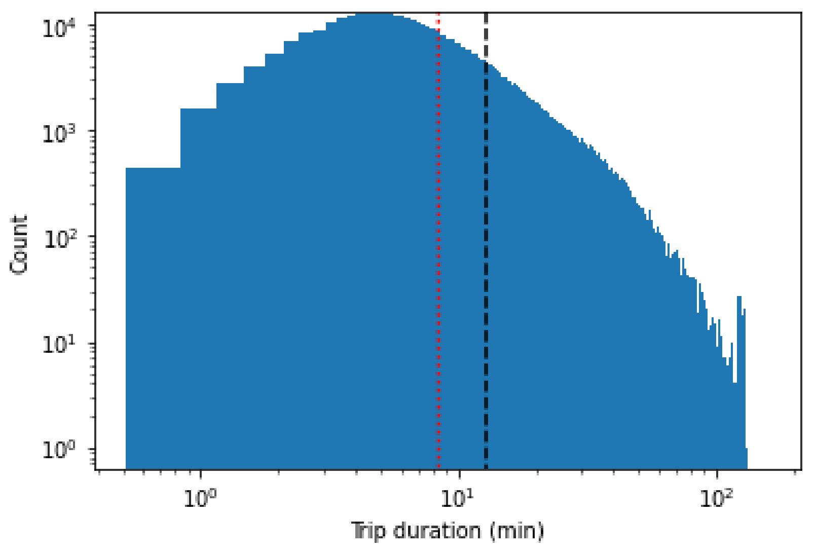
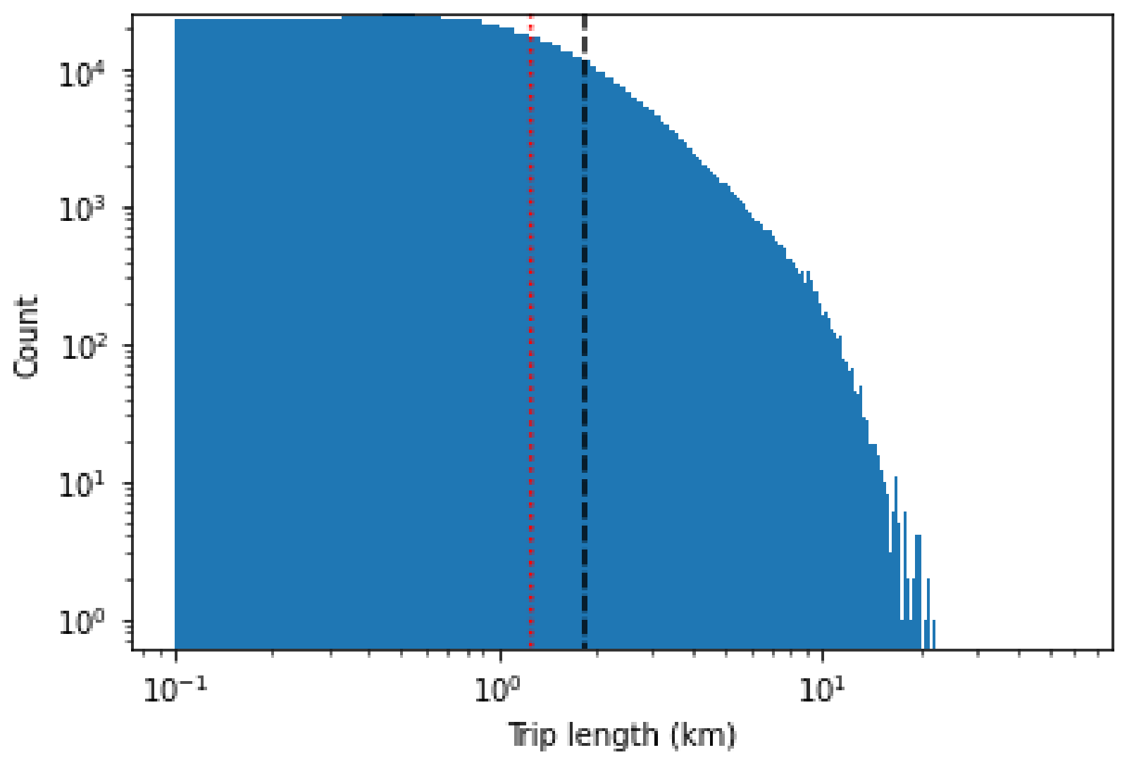
2.1. Dataset

In July 2019, a shared e-scooter service was introduced to Calgary, Canada with the companies Lime deploying 1000 and Bird deploying 500 scooters. The City of Calgary provided us with a dataset of e-scooter usage over a period of 75 days from 15 July 2019 to 27 September 2019. Calgary covers an area of 825 km2 with its population of 1,285,711. The shared e-scooter service is dockless, i.e., there are no designated parking stations. A user can rent and return the e-scooter at any location using a mobile app. Each time an e-scooter was rented, its usage information was recorded, from which the data available to us included the date, hour (hour of the day in which the scooter was rented), day of the week, trip duration (in minutes), trip length (in kilometers), and starting/ending geolocations (latitude, longitude). To protect data privacy, the starting and ending geolocations were normalized by the City into 300-m2 hexagonal grids.
Data included 459,478 total e-scooter rides from 4901 different starting grid locations to 5242 ending grid locations. Average demand for each day of the week is shown in Figure 1, where the demand rises from Monday to Wednesday then drops slightly and rises again and drops on Sunday. Saturday has the highest average daily demand, which was presumably generated largely by weekend recreational trips. When considering hourly demand, Figure 2 shows the overall average demand as well as demand across each day of the week. Overall, the demand begins to rise from 5 a.m. then drops down slightly during the 9 a.m. hour, rises to a peak during the 4 p.m. hour, then gradually drops to the lowest level during the 4 a.m. hour. The morning peak (6 a.m.–8 a.m.) is only observed for weekdays, which is most likely due to daily commuting to work.
On average, each trip lasted for 12.84 min and traveled for 1.85 km, where the trip duration and trip length distributions are shown in Figure 3 and Figure 4, respectively. Distributions are plotted using a logscale because they seemingly follow a long tail distribution and so they are more observable on a logscale. There were 166,271 trips and over one-third of all trips (36.19%), were less than 1 km. For these short distances, e-scooters may replace walking rather than driving as observed and discussed in [28,45].
Geographically, e-scooter demand was mostly seen in the city center area and along the public transit stations for light rail and bus. Overall spatial distribution of e-scooter demand as well as aggregated demand for each day of the week across the city of Calgary are shown in Figure 5, where brighter color implies higher demand and green dots indicate public transit station locations. Peripheral demand took place mostly over the weekend, especially in the Northwest area of the city where there is a recreational flow along the Bow River.

2.2. Predictive Model

Our approach to scooter demand prediction was to consider spatial demand density as an image. With the same spatial coordinates, a prediction can be made based on a series of historical demand densities (density maps). This approach allows us to take advantage of a machine learning technique used in computer vision called the fully convolutional network or FCN [46], which is a deep learning model typically used for image segmentation. Taking a similar approach to the image segmentation, the output of the FCN is the predicted spatial demand instead of class confidence. FCN was chosen over the conventional convolutional neural network, or CNN [47], because FCN performs a pixel-wise operation, so that it does not contain fully connected layers. Hence, the output of the FCN can be an image of the same size as the input images rather than an image class, as produced by a CNN. Technically, the CNN is used for classification of the whole images, i.e., identifying a class of them, while the FCN, on the other hand, is used for a pixel-wise classification i.e., determining a class of each pixel. Hence, the FCN is more suitable for spatial and temporal correlated data points, which can be considered as image pixels of spatial demand in our case.
FCN based network architectures have the proven ability of learning spatial patterns in image segmentation tasks or temporal patterns in flow estimation tasks [48]. The number of required parameters for training FCNs is not high. Hence, they can be trained quite fast. Therefore, they are highly flexible to the application of any geographical-based masks to the FCN model as additional information. Since the network is not deep, the image size is not large in our scenario and we wanted to retain the output’s resolution, we chose not to use the pooling layers as in the standard FCN, or upsampling layers and skip connections as in the U-Net [49], or unpooling layers with pooling indices as in the SegNet [50].

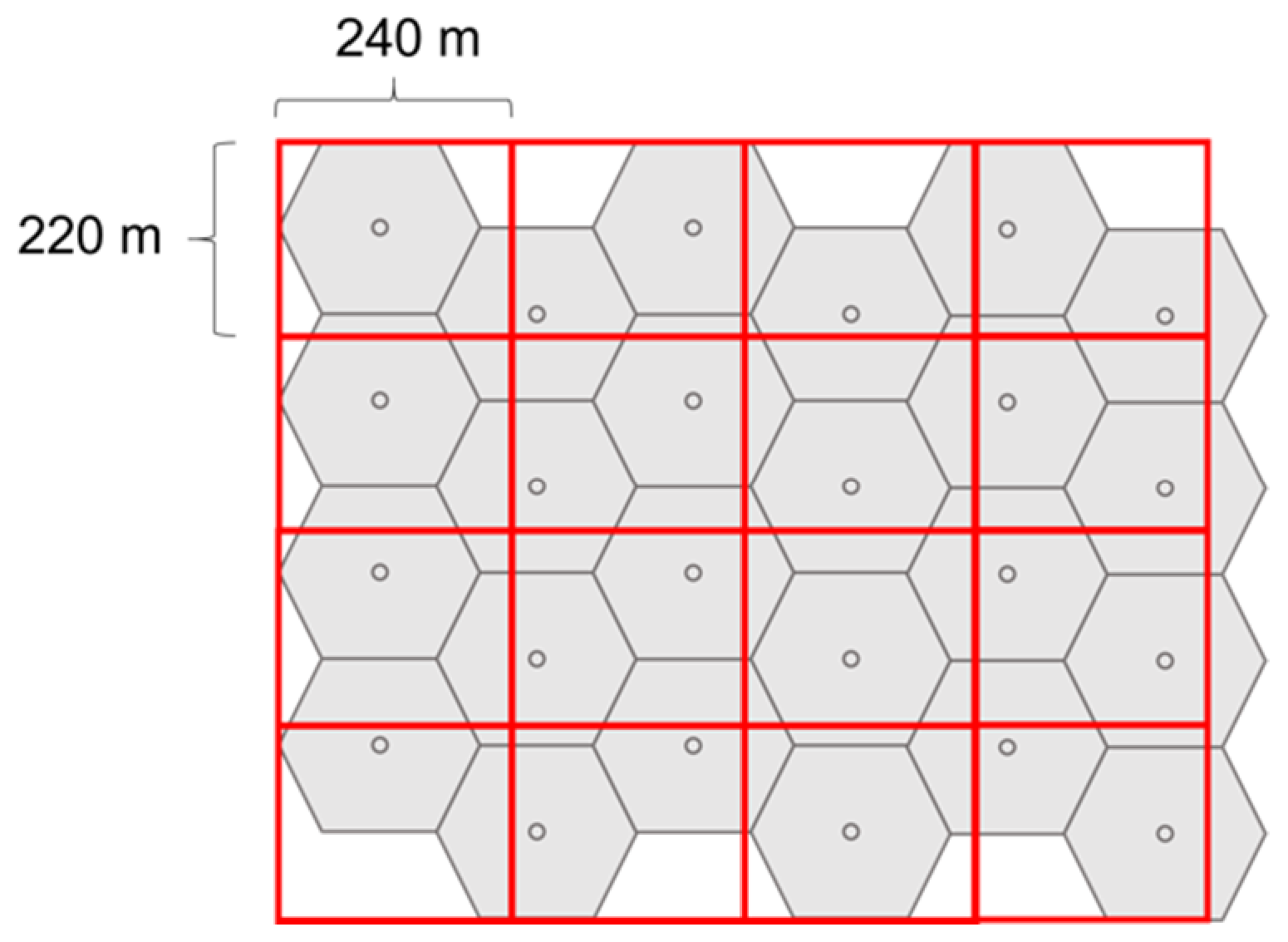
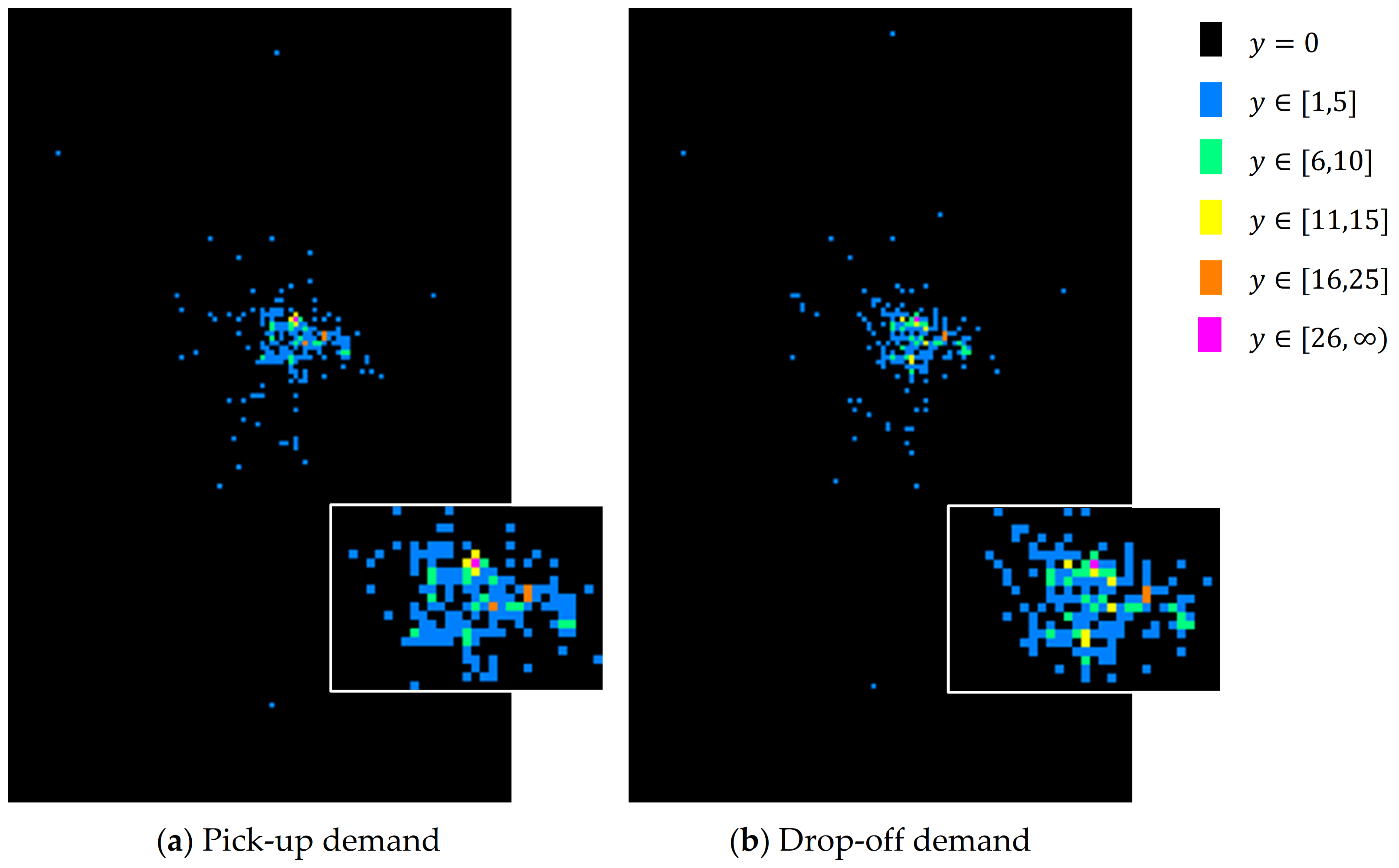
2.2.1. Data Preparation

In the initial step, our spatial demand information must be prepared into a form of image, so that it can be fed into the FCN model. The standard convolutional layers in the neural networks are defined based on a cartesian coordinate system (discrete) and the input/output data is stored in a 3D array system. Therefore, in order to use the standard libraries for implementing convolutional layers to neural networks, we needed to transform the demand data from the original hexagonal grids to rectangular grids. The original 300-m2 hexagonal grids were therefore mapped onto 220 × 240-m2 rectangular grids where any demands associated with the hexagonal grids were transferred into the newly assigned grids, as shown in Figure 6, which is still within a reasonable walking distance, reachable within 5 min by foot given an average walking speed of 1.47 m/s [51]. However, the proposed methodology is applicable to other grid sizes. Spatial demand can then be plotted on an image of size 167 × 106 pixels that covers all scooter demand in the city of Calgary.
With the rectangular grids, sample images of density maps reflecting pick-up and drop-off demand levels (distinguished by color) during 2–3 p.m. on Sunday, 28 July 2019, are shown in Figure 7.

2.2.2. Global Masking

A global mask (shown in Figure 8) was created to guide the FCN to focus on only pixels with potential demand based on the entire past demands, so that the model only learns and predicts within the masked area or region of interest (ROI). The ROI was generated according to Equation (1).
R O I i , j = 1 t p i , j , t + d i , j , t > 0 0 o t h e r w i s e
where p i , j , t and d i , j , t are pick-up and drop-off demands at position i , j , at time t . ROI value at grid (i, j) or R O I i , j is set to one if there exits at least one demand (pick-up or drop-off) in that grid in the previous record and is set to zero if there is no demand in that grid in the previous record. This ROI scheme can also be applied in other scenarios besides our case, such as value assignment based on other geographical or area information, e.g., physical environments, urban settings, and so on.

2.2.3. Feature Selection

As human mobility has a high degree of temporal and spatial regularity [52], our approach to feature selection was to select spatial demand densities (in the form of images) that correlate well with the predicted period. So, the absolute differences and average correlation coefficients between pick-up and drop-off demands for time difference k are calculated as follows.
A D S k = i , j     R O I t     T R A I N p i , j , t p i , j , t k + i , j     R O I t     T R A I N d i , j , t d i , j , t k
A D C k = i , j     R O I t     T R A I N p i , j , t d i , j , t k + i , j     R O I t     T R A I N d i , j , t p i , j , t k
where A D S k and A D C k are absolute differences in demands at time difference k in hour units, R O I is a set of the positions i , j where R O I i , j = 1 , and T R A I N is a set of the time in the training set.
C O R R S k = 1 2 R p t , p t k + R d t , d t k
C O R R C k = 1 2 R p t , d t k + R d t , p t k
where C O R R S k and C O R R C k are the average correlation coefficients of the demands at time difference k , and R a , b represents a Pearson correlation coefficient between variables a and b.
Features were selected among varying values of k based on A D S ,   A D C ,   C O R R S ,   and C O R R C . The values of k that produce the top 20 lowest A D S and A D C , and the top 20 highest C O R R S and C O R R C were considered and selected as the input feature map. Table 1 shows the selected features from the varying k values for two prediction schemes: next hour or t + 1 prediction and next 24-h or t + 24 prediction. Intuitively, there are high correlations between the next hour demand and the immediate previous demands like the current (t − 0) and last hour (t − 1) demands, as well as yesterday’s same hours i.e., (t − 22), (t − 23), (t − 24), and last week’s similar hours, i.e., (t − 143), (t − 166), (t − 167), and (t − 143), for instance. The same presumption can be made for the next 24-h demands. Thereby, those highly correlated demand hours are listed in Table 1. Both prediction schemes can be useful for scooter operational management for a short-term as well as long-term planning.

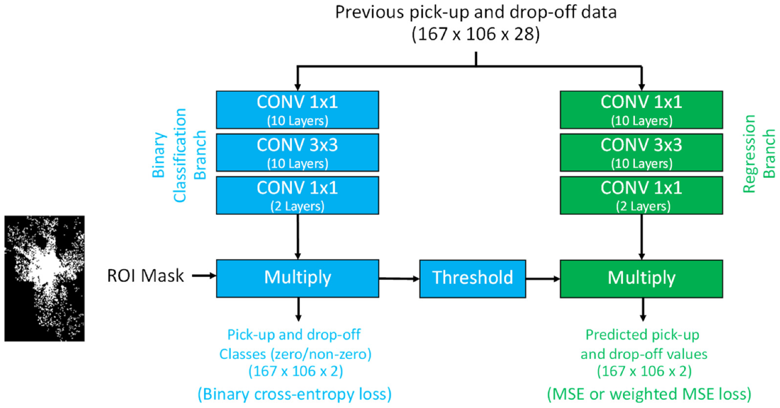
2.2.4. Network Architecture

We modified the FCN model by adding the masking process to better guide the model, and hence developed a new network architecture, namely, the Masked Fully Convolutional Network (MFCN), as shown in Figure 9. The input of the MFCN is a series of historical pick-up and drop-off demand density images (maps) at time t k as shown in the Table 1, totally 28 feature maps.
There is no pooling layer in the network in order to keep the resolution of the output as the input’s size. The network consists of two branches: regression and classification. The regression branch is for predicting a demand image or map. Since the demand map consists of a large number of zeros (after the global mask is applied), the classification branch is applied to mask these zero values, as a local mask, i.e., the time-variant mask. The output of the classification branch is pick-up or drop-off demand class map (with some confidence level from 0–1.0), which will then be quantized to 0 or 1 by the threshold value of 0.5 (where 0 implies zero demand and 1 implies non-zero demand). The output of the regression branch is a map with predicted spatial demand values.
The thresholding and multiplying layers are there to allow only some masked pixels to influence weight updating in the regression branch, i.e., reducing the effect of zero-demand pixels. The multiply layer is an elementwise operation, i.e., producing an entry-wise product. The number of convolutional layers, the number of feature maps in each layer, and the size of the filters can be modified based on how much spatial correlation spreads to the neighboring pixels in a given demand prediction problem. In our case, we used a 1 × 1 filter for the first convolutional layer to reduce the dimension of the input (i.e., the number of input feature maps) from 28 to 10, so that it consequently reduced the number of trainable parameters. A 3 × 3 filter was used for the next convolutional layer for modeling the spatial relation between the pixels and their adjacent pixels. Finally, a 1 × 1 filter was used for the last convolutional layer to decode the feature map (i.e., outputs of the previous layer) into the pick-up and drop-off demand values/classes.

2.2.5. Loss Function

To optimize our prediction by minimizing the error, a loss function is used as another important component of our MFCN model. Loss is simply a prediction error that is used to calculate the gradients, which are then used to update the weights of the MFCN. This is how our network is trained. The loss function is defined as follows.
e = w y y ^ y 2 + γ m ^ log m + 1 m ^ log 1 m
where y and y ^ are the actual demand in each position and its prediction (including pick-up and drop-off demands) in the regression branch, m and m ^ are the actual active class (i.e., zero or non-zero demands) in each position and its prediction (including pick-up and drop-off demands) in the binary classification branch, and γ is a weight for scaling the errors between weighted mean squared error (WMSR) and binary cross entropy, where
w y = 1 y y 2   for   unweighted   MSE   for   the   first   order   weighted   MSE     for   the   sec ond   degree   order   weighted   MSE
Therefore, the total loss is the sum of the regression loss from the regression branch and the binary cross entropy loss from the classification branch.

3. Results

To evaluate our MFCN model for both prediction schemes (i.e., next-hour and next 24-h predictions), we used the first 61 days of scooter data for training the model and the last 14 days for testing. We compared the performance of our proposed MFCN model against three baseline models. The first baseline is a naïve forecasting, which simply predicts the demand to be the same as the previous occurrence, i.e., predicting the next hour demand ( y ^ t + 1 ) to be the same as the last hour demand ( y t ) for instance. The second baseline is the linear regression model [53] trained with the same set of data as our model and the same selected features listed in Table 1. The third baseline is the e-scooter prediction model proposed by Ham et al. [8], which is based on the autoencoder and convolutional long short-term memory (LSTM) network, also trained with the same training set. For the Ham et al. model, three different sets of the number of hidden states were examined (i.e., 100, 200, and 300 states) from which the model performed best with 200 hidden states, and hence this setup was used for our comparative analysis. The mean absolute error (MAE) and max absolute error (Max AE) were used for the performance measurement and comparison between the models and are defined by Equations (8) and (9), respectively.
M A E = i = 1 n y i y ^ i n
M a x   A E = max i 1 , 2 , ,   n y i y ^ i
The performance of all models when used for the next-hour demand prediction is shown in Table 2, which includes the detail on the associated loss function used, the size of features, the number of parameters, and the values of MAE and Max AE for different levels of demand as well as the overall demand (i.e., entire ROI). Higher populated areas are likely to be associated with higher levels of demand; however, this doesn’t mean that a lower demand areas are not important, as the scooter operator ideally wants to provide the right amount of service in all areas. Therefore, the model performance was thus evaluated across different levels of demand throughout the service area. Our proposed MFCN model was examined with three different loss functions to observe the effect of weighting in model penalization through the loss function (i.e., the higher the order, the greater penalty in model learning). For visibility in reading the result in Table 2, the lowest error value in each column is highlighted in bold. Overall, when considering the overall demand across the entire ROI, the proposed MFCN with MSE loss function performs best with MAE of 0.0434. Recognizing areas with zero demand is also critical for the scooter operator in scooter dispatching, so zero demand prediction (y = 0) was experimented. As a result, our MFCN with MSE has the best performance with MAE = 0.0057 and Max AE = 8.0060. For the non-zero demand prediction (y > 0), the proposed MFCN with MSE also has the best performance with MAE = 1.5180. When different levels of demand are considered, the MFCN with MSE is the best predictor with MAE = 1.2136 and Max AE = 11.4640 for the demand ranging from 1–5 scooters, i.e., y  [1,5], mostly located in the outskirts of the city. However, it is interesting and intuitive to observe that when the demand gets higher, or in the other words, as we get closer to the city center, the MFCN with a higher-order WMSE loss function performs better, and is the best among other compared models. Therefore, it is reasonable to suggest that the proposed MFCN is the most suitable model for the next-hour pick-up demand prediction where its associated loss function (MSE or WMSE) can be chosen in relation to the targeted demand level, which is often linked to the service area.
The next-hour prediction of drop-off demand was also tested in the same way as the pick-ups since being able to recognize drop-off demand also helps the scooter operator in their proactive scooter dispatching process. A similar result was observed when considering the entire ROI, zero demand, and non-zero demand, that the MSCN with MSE loss function has the best performance (see Table 3). The regression model beats our MFCN with MSE by 0.0156 scooters in MAE for the [1,5]-demand level. From the demand level of at least six scooters, the proposed MFCN with WMSE has the best performance by producing similar results in the pick-up prediction, i.e., the higher order of WMSE yields a better performance for higher demand levels. Consequently, a similar suggestion to the pick-up demand prediction can be made here that for the next-hour drop-off demand prediction the MFCN model is the most suitable predictor, except for the [1,5]-demand level as the linear regression tends to perform slightly better.
Our MFCN model outperforms the Ham et al. model [8], which is the state of the art in e-scooter demand prediction. The dense connection in the LSTM’s layers of the Ham et al. model requires a large number of trainable parameters. Although dense connection allows the network to learn the relation between each output and input pixel throughout the image, high correlation is mostly found between the neighboring pixels in the case of scooter demand prediction. Another shortcoming of the Ham et al. model is that its prediction is based only on a few previous demand values (i.e., LSTM with five steps). However, the demand during time t + 1 is highly correlated not only with the demands in the previous few timestamps but also the same time a day earlier ( t 23 ) and the same time a week earlier ( t 167 ), as our model has taken into account (features listed in Table 1). So, the feature selection process described in our methodology could be applied to potentially improve its prediction performance. The feature selection process has shown its significant impact as evidenced by seeing that a simple linear regression model outperforms a much more sophisticated model like Ham et al.’s by using the features listed in Table 1. Another potential improvement on the Ham et al. model is to use a CNN over its recurrent neural network (RNN) to allow the model to pay attention to each previous time step equally. To cope with the spare input, the Ham et al. model uses the autoencoder to compress the input image into latent features, while our MFCN model uses the masking process and weighted loss function. Using the weighted loss function enables us to shape the loss distribution more effectively.
The overall performance of the proposed MFCN model in terms of the average prediction error (MAE) for the next-hour prediction scheme for both pick-up and drop-off demands is shown in Figure 10. It can be observed that the error rises on Monday and Saturday. This is due to the fact that the model takes the same set of selected features (listed in Table 1) for all predictions made, regardless of the day type, i.e., weekday, weekend, holiday, and so on. Consideration of different sets of selected features based on day type can potentially improve the performance of the MFCN model, which is worth future research for the model’s further improvement.
In addition to the next-hour demand prediction, we also conducted an experiment on the next 24-h prediction for both pick-up and drop-off demands. In this prediction scheme, the Ham et al. model was not included in our experiment as their model was designed only for next-hour predictions. The result of the pick-up demand prediction is shown in Table 4. A similar trend in model performance with the next-hour prediction is also observed here in the next 24-h prediction scheme. Our MFCN model without weighted loss function has the best performance overall (ROI, y = 0, and y > 0). Yet, when different levels of demand were considered, the MFCN without weighted loss function has the best MAE for only the [1,5]-demand level, while the MFCN with first order weighted loss function outperforms other models for the demand ranging from 6 to 15 scooters. As the demand level becomes even larger, the MFCN with second order weighted loss function (i.e., greater penalty in model learning) intuitively emerges as the best predictor for pick-up demand of greater than 16 scooters, which is often seen around the city center area.
The next 24-h drop-off prediction experiment was conducted in a similar way, the results of which are shown in Table 5. The MFCN with MSE has the best performance overall (ROI) as well as for zero-demand prediction (y = 0). Interestingly, the linear regression outperforms the MSCN with MSE by 0.0618 scooters for positive demand (y > 0) prediction. The linear regression also performs well for the [1,5]-demand level with MAE of 1.2385. The MFCN with first order WMSE is the best predictor for [6, 10]-demand level, while the MFCN with second order WMSE outperforms other models for all other greater demand levels (from 11 scooters onwards).
As an overall performance of our MFCN model, average prediction error in terms of MSE loss in each hour and each day of the week for the next 24-h prediction scheme for both pick-up and drop-off demands is shown in Figure 11. A similar trend is also observed in this prediction scheme where error jumps on Monday and Saturday, which is due to the aforementioned non-consideration of day type. The MFCN model has higher average error in the next 24-h prediction scheme than the next-hour prediction scheme, which is intuitive. Specifically, the next 24-h prediction scheme has 0.167 and 0.0848 higher errors than the next-hour prediction scheme for the pick-up and drop-off demand predictions, respectively.
Overall, our MFCN performs better as a pick-up demand predictor than a drop-off demand predictor in terms of the error. Since the next-hour demand is likely to be intuitively easier to predict than looking farther into the future like next 24 h, so our MFCN model performs better for the next hour demand prediction than the next 24-h prediction. In summary, the MFCN model outperforms other baselines in all cases considered for pick-up demand prediction for both schemes. For drop-off demand prediction, the MFCN performs better than other baselines except for the next-hour prediction where demand is low (i.e., y  [1,5]), and for the next 24-h drop-off demand prediction where only positive demands are concerned (y > 0) and low-level demand (y  [1,5]) is of interest for which a linear regression performs slightly better. As seen in the experimental result, the proposed MFCN model can be used with a different loss function depending upon the demand level of interest. Using MFCN with a higher-degree weighted loss function is more suitable for areas with greater demand levels, such as the city center. Since all levels of demand are equally important for the e-scooter operator as they seek to balance supply and demand, with our MFCN model three choices of a loss function are available to choose from.

4. Conclusions

Provided as a dockless service, e-scooters are more flexible to use than other dock-based micromobility services such as e-bikes that often require pick-up and drop-off stations [54]. Dock-based shared mobility services face imbalances in the system at selected locations in a city (e.g., bike station). However, the dockless system faces a challenge of imbalances that cannot be measured at selected points in space, which is more widespread. The e-scooter demand is aggregated at a zonal level, which was represented by a 220 m by 240 m grid. Therefore, grid-level demand anticipation or being able to accurately predict spatiotemporal demand of e-scooter usage was seen as one of the rebalancing strategies. In this work, we developed a predictive model for pick-up and drop-off demands based on a fully convolutional network. Like other urban public transit services, the demand for e-scooters varies with area type, population density, rider behavior, and countless other factors [55]. Subsequently, e-scooter usage is sparse, i.e., most of the demand appears around the city center and the rest spreads out through other parts of the town. Therefore, our model tackles the sparsity of the e-scooter data with its masking process and weighted loss function, and so the model is named after its core components as the masked fully convolutional network or MFCN. The proposed MFCN model has been evaluated in terms of prediction error against other baseline models including naïve forecasting (based only on a previous value), linear regression, and LSTM network with autoencoder [8]. The experimental results show that our MFCN has the best performance overall for pick-up demand prediction in both prediction schemes; next-hour and next 24-h demands. The mean absolute errors of the next-hour prediction are 0.0434 and 0.0464 for pick-up and drop-off demands respectively, while the errors of the next 24-h prediction are 0.0491 and 0.0501, respectively.
The MFCN model can play a useful role for e-scooter service providers in their supply–demand balancing strategies that seek to leverage the anticipation of both pick-up and drop-off spatiotemporal demands in the serviced area. Nonetheless, there are a few limitations of the current development of the MFCN model which could be considered in its future improvement. Firstly, the model could benefit from the sequential training scheme with which the model gets trained once a new data stream arrives or once each prediction is validated. Secondly, a set of different training–testing data portions could potentially be explored for a more rigorous performance evaluation, which could lead to another interesting research question of adequacy of training data [56]. Lastly, the model could benefit from taking into account the day type, i.e., weekday, weekend, or holiday for which different sets of influential features may be used. Other future research directions include e-scooter origin–destination (O–D) estimation, visual analytics tools for e-scooter operational monitoring and analysis, and urban traffic modeling and characterization using e-scooter usage information.

Author Contributions

Conceptualization, Santi Phithakkitnukooon and Merkebe Getachew Demissie; methodology, Karn Patanukhom; validation, Karn Patanukhom; formal analysis, Santi Phithakkitnukooon and Karn Patanukhom; investigation, Santi Phithakkitnukooon, Merkebe Getachew Demissie, and Karn Patanukhom; resources, Merkebe Getachew Demissie; data curation, Karn Patanukhom; writing—original draft preparation, Santi Phithakkitnukooon, Merkebe Getachew Demissie and Karn Patanukhom; writing—review and editing, Santi Phithakkitnukooon, Merkebe Getachew Demissie, and Karn Patanukhom; visualization, Santi Phithakkitnukooon and Karn Patanukhom. All authors have read and agreed to the published version of the manuscript.

Funding

This work is partially funded by the Schulich School of Engineering, University of Calgary Startup Grant.

Data Availability Statement

The data used in this study cannot be made publicly available due to commercial reasons. However, we can make a sample of data available to other researchers upon request.

Acknowledgments

We would like to thank the City of Calgary for providing e-scooter service usage data for this research.

Conflicts of Interest

The authors declare no conflict of interest.

References

  1. Gössling, S. Integrating E-Scooters in Urban Transportation: Problems, Policies, and the Prospect of System Change. Transp. Res. Part D Transp. Environ. 2020. [Google Scholar] [CrossRef]
  2. McKenzie, G. Spatiotemporal Comparative Analysis of Scooter-Share and Bike-Share Usage Patterns in Washington, D.C. J. Transp. Geogr. 2019, 78, 19–28. [Google Scholar] [CrossRef]
  3. Chang, A.Y.; Miranda-Moreno, L.; Clewlow, R.; Sun, L. Trend or Fad? Deciphering the Enablers of Micromobility in the U.S.; SAE International: Warrendale, PA, USA, 2019. [Google Scholar]
  4. Hosseinzadeh, A.; Algomaiah, M.; Kluger, R.; Li, Z. E-Scooters and Sustainability: Investigating the Relationship between the Density of E-Scooter Trips and Characteristics of Sustainable Urban Development. Sustain. Cities Soc. 2020, 66, 102624. [Google Scholar] [CrossRef]
  5. Sedor, A.; Oriold, J. Shared E-Bike and E-Scooter Final Pilot Report. In Proceedings of the SPC on Transportation and Transit, Calgary, AL, Canada, 16 December 2020. [Google Scholar]
  6. Fearnley, N.; Johnsson, E.; Berge, S.H. Patterns of E-Scooter Use in Combination with Public Transport. Findings 2020. [Google Scholar] [CrossRef]
  7. Moreau, H.; de Jamblinne de Meux, L.; Zeller, V.; D’Ans, P.; Ruwet, C.; Achten, W.M.J. Dockless E-Scooter: A Green Solution for Mobility? Comparative Case Study between Dockless e-Scooters, Displaced Transport, and Personal e-Scooters. Sustainability 2020, 12, 1803. [Google Scholar] [CrossRef] [Green Version]
  8. Ham, S.W.; Cho, J.-H.; Park, S.; Kim, D.-K. Spatiotemporal Demand Prediction Model for E-Scooter Sharing Services with Latent Feature and Deep Learning. Transp. Res. Rec. 2021, 1–10. [Google Scholar] [CrossRef]
  9. Abduljabbar, R.L.; Liyanage, S.; Dia, H. The Role of Micro-Mobility in Shaping Sustainable Cities: A Systematic Literature Review. Transp. Res. Part D Transp. Environ. 2021, 92, 102734. [Google Scholar] [CrossRef]
  10. Palm, M.; Farber, S.; Shalaby, A.; Young, M. Equity Analysis and New Mobility Technologies: Toward Meaningful Interventions. J. Plan. Lit. 2021, 36, 31–45. [Google Scholar] [CrossRef]
  11. Abdelwahab, B.; Palm, M.; Shalaby, A.; Farber, S. Evaluating the Equity Implications of Ridehailing through a Multi-Modal Accessibility Framework. J. Transp. Geogr. 2021, 95, 103147. [Google Scholar] [CrossRef]
  12. Boarnet, M.G.; Giuliano, G.; Hou, Y.; Shin, E.J. First/Last Mile Transit Access as an Equity Planning Issue. Transp. Res. Part A Policy Pract. 2017, 103, 296–310. [Google Scholar] [CrossRef]
  13. Szmelter, A. Mobility-as-a-Service—A Challenge for It in the Age of Sharing Economy. Inf. Syst. Manag. 2018, 7, 59–71. [Google Scholar] [CrossRef]
  14. Herrmann, T.; Gleckner, W.; Wasfi, R.A.; Thierry, B.; Kestens, Y.; Ross, N.A. A Pan-Canadian Measure of Active Living Environments Using Open Data. Heal. Rep. 2019, 30, 16–25. [Google Scholar] [CrossRef]
  15. Hermosilla, T.; Palomar-Vázquez, J.; Balaguer-Beser, Á.; Balsa-Barreiro, J.; Ruiz, L.A. Using Street Based Metrics to Characterize Urban Typologies. Comput. Environ. Urban Syst. 2014, 44, 68–79. [Google Scholar] [CrossRef] [Green Version]
  16. Jiao, J.; Bai, S. Understanding the Shared E-Scooter Travels in Austin, TX. ISPRS Int. J. Geo-Inf. 2020, 9, 135. [Google Scholar] [CrossRef] [Green Version]
  17. Almannaa, M.H.; Ashqar, H.I.; Elhenawy, M.; Masoud, M.; Rakotonirainy, A.; Rakha, H. A Comparative Analysis of E-Scooter and E-Bike Usage Patterns: Findings from the City of Austin, TX. arXiv 2020, arXiv:2006.04033. [Google Scholar] [CrossRef]
  18. Le Figaro Trottinettes: La Mairie de Paris Veut Une Réglementation Nationale. Available online: http://www.lefigaro.fr/flash-eco/2018/09/09/97002-20180909FILWWW00064-trottinettes-la-mairie-de-paris-veut-une-reglementation-nationale.php (accessed on 28 December 2020).
  19. Times, L.A. Approves Rules for Thousands of Scooters, with a 15-Mph Speed Limit and Aid for Low-Income Riders. Available online: https://www.latimes.com/local/lanow/la-me-ln-scooter-vote-20180904-story.html (accessed on 22 December 2020).
  20. Seattle Department of Transportation Seattle Department of Transportation (SDOT) Response to City Council Resolution 31898, Requesting That the Seattle Department of Transportation Develop a Budget Proposal for Creating on-Street Bike and e-Scooter Parking. Available online: http://clerk.seattle.gov/search/clerk-files/321445 (accessed on 27 December 2020).
  21. Streets Blog LA Santa Monica Installs In-Street E-Scooter Parking Corrals. Available online: https://la.streetsblog.org/2018/11/08/santa-monica-installs-in-street-e-scooter-parking-corrals/ (accessed on 27 December 2020).
  22. Fanchao, L.; Gonçalo, C. Electric Carsharing and Micromobility: A Literature Review on Their Usage Pattern, Demand, and Potential Impacts. Int. J. Sustain. Transp. 2020, 1–30. [Google Scholar] [CrossRef]
  23. Hardt, C.; Bogenberger, K. Usage of E-Scooters in Urban Environments. Transp. Res. Procedia 2019, 37, 155–162. [Google Scholar] [CrossRef]
  24. Portland Bureau of Transportation. 2018 E-Scooter Findings Report; Portland Bureau of Transportation: Portland, OR, USA, 2019. [Google Scholar]
  25. Bai, S.; Jiao, J. Dockless E-Scooter Usage Patterns and Urban Built Environments: A Comparison Study of Austin, TX, and Minneapolis, MN. Travel Behav. Soc. 2020, 20, 264–272. [Google Scholar] [CrossRef]
  26. Caspi, O.; Smart, M.J.; Noland, R.B. Spatial Associations of Dockless Shared E-Scooter Usage. Transp. Res. Part D Transp. Environ. 2020, 86, 102396. [Google Scholar] [CrossRef]
  27. Trivedi, T.K.; Liu, C.; Antonio, A.L.M.; Wheaton, N.; Kreger, V.; Yap, A.; Schriger, D.; Elmore, J.G. Injuries Associated With Standing Electric Scooter Use. JAMA Netw. Open 2019, 2, e187381. [Google Scholar] [CrossRef]
  28. James, O.; Swiderski, J.I.; Hicks, J.; Teoman, D.; Buehler, R. Pedestrians and E-Scooters: An Initial Look at e-Scooter Parking and Perceptions by Riders and Non-Riders. Sustainability 2019, 11, 5591. [Google Scholar] [CrossRef] [Green Version]
  29. Hollingsworth, J.; Copeland, B.; Johnson, J.X. Are E-Scooters Polluters? The Environmental Impacts of Shared Dockless Electric Scooters. Environ. Res. Lett. 2019, 14, 084031. [Google Scholar] [CrossRef]
  30. Balsa-Barreiro, J.; Valero-Mora, P.M.; Menéndez, M.; Mehmood, R. Extraction of Naturalistic Driving Patterns with Geographic Information Systems. Mob. Netw. Appl. 2020, 1–17. [Google Scholar] [CrossRef]
  31. Montero, L.; Codina, E.; Barceló, J. Dynamic OD Transit Matrix Estimation: Formulation and Model-Building Environment. In Advances in Intelligent Systems and Computing; Springer: New York, NY, USA, 2015. [Google Scholar]
  32. Kaeoruean, K.; Phithakkitnukoon, S.; Demissie, M.G.; Kattan, L.; Ratti, C. Analysis of Demand–Supply Gaps in Public Transit Systems Based on Census and GTFS Data: A Case Study of Calgary, Canada. Public Transp. 2020, 12, 483–516. [Google Scholar] [CrossRef]
  33. Prommaharaj, P.; Phithakkitnukoon, S.; Demissie, M.G.; Kattan, L.; Ratti, C. Visualizing Public Transit System Operation with GTFS Data: A Case Study of Calgary, Canada. Heliyon 2020, 6, e03729. [Google Scholar] [CrossRef]
  34. Demissie, M.G.; Phithakkitnukoon, S.; Sukhvibul, T.; Antunes, F.; Gomes, R.; Bento, C. Inferring Passenger Travel Demand to Improve Urban Mobility in Developing Countries Using Cell Phone Data: A Case Study of Senegal. IEEE Trans. Intell. Transp. Syst. 2016, 17, 2466–2478. [Google Scholar] [CrossRef]
  35. Hankaew, S.; Phithakkitnukoon, S.; Demissie, M.G.; Kattan, L.; Smoreda, Z.; Ratti, C. Inferring and Modeling Migration Flows Using Mobile Phone Network Data. IEEE Access 2019, 7, 164746–164758. [Google Scholar] [CrossRef]
  36. Demissie, M.G.; Phithakkitnukoon, S.; Kattan, L. Trip Distribution Modeling Using Mobile Phone Data: Emphasis on Intra-Zonal Trips. IEEE Trans. Intell. Transp. Syst. 2019, 20, 2605–2617. [Google Scholar] [CrossRef]
  37. Soliman, A.; Soltani, K.; Yin, J.; Padmanabhan, A.; Wang, S. Social Sensing of Urban Land Use Based on Analysis of Twitter Users’ Mobility Patterns. PLoS ONE 2017, 12, e0181657. [Google Scholar] [CrossRef] [PubMed] [Green Version]
  38. Ke, J.; Zheng, H.; Yang, H.; Chen, X. Short-Term Forecasting of Passenger Demand under on-Demand Ride Services: A Spatio-Temporal Deep Learning Approach. Transp. Res. Part C Emerg. Technol. 2017, 85, 591–608. [Google Scholar] [CrossRef] [Green Version]
  39. Wang, C.; Hou, Y.; Barth, M. Data-Driven Multi-Step Demand Prediction for Ride-Hailing Services Using Convolutional Neural Network. In Advances in Computer Vision; Springer: New York, NY, USA, 2020. [Google Scholar]
  40. Demissie, M.G.; Kattan, L.; Phithakkitnukoon, S.; Homem de Almeida Correia, G.; Veloso, M.; Bento, C. Modeling Location Choice of Taxi Drivers for Passenger Pick-Up Using GPS Data. IEEE Intell. Transp. Syst. Mag. 2020, 70–90. [Google Scholar] [CrossRef]
  41. Mungthanya, W.; Phithakkitnukoon, S.; Demissie, M.G.; Kattan, L.; Veloso, M.; Bento, C.; Ratti, C. Constructing Time-Dependent Origin-Destination Matrices with Adaptive Zoning Scheme and Measuring Their Similarities with Taxi Trajectory Data. IEEE Access 2019, 7, 77723–77737. [Google Scholar] [CrossRef]
  42. Kunama, N.; Worapan, M.; Phithakkitnukoon, S.; Demissie, M. GTFS-VIZ: Tool for Preprocessing and Visualizing GTFS Data. In UbiComp/ISWC 2017, Proceedings of the 2017 ACM International Joint Conference on Pervasive and Ubiquitous Computing and Proceedings of the 2017 ACM International Symposium on Wearable Computers, Maui, Hawaii, 11–17 September 2017; Association for Computing Machinery: New York, NY, USA, 2017. [Google Scholar]
  43. Kinjarapu, A.; Demissie, M.G.; Kattan, L.; Duckworth, R. Applications of Passive GPS Data to Characterize the Movement of Freight Trucks—A Case Study in the Calgary Region of Canada. IEEE Trans. Intell. Transp. Syst. 2021, 1–16. [Google Scholar] [CrossRef]
  44. Mei, B. Destination Choice Model for Commercial Vehicle Movements in Metropolitan Area. Transp. Res. Rec. 2013, 2344, 126–134. [Google Scholar] [CrossRef]
  45. Sanders, R.L.; Branion-Calles, M.; Nelson, T.A. To scoot or not to scoot: Findings from a recent survey about the benefits and barriers of using E-scooters for riders and non-riders. Transp. Res. Part A Policy Pract. 2020, 139, 217–227. [Google Scholar] [CrossRef]
  46. Shelhamer, E.; Long, J.; Darrell, T. Fully Convolutional Networks for Semantic Segmentation. IEEE Trans. Pattern Anal. Mach. Intell. 2017, 39, 640–651. [Google Scholar] [CrossRef]
  47. Sultana, F.; Sufian, A.; Dutta, P. Evolution of Image Segmentation Using Deep Convolutional Neural Network: A Survey. Knowl.-Based Syst. 2020, 201–202, 1–25. [Google Scholar] [CrossRef]
  48. Dosovitskiy, A.; Fischery, P.; Ilg, E.; Hausser, P.; Hazirbas, C.; Golkov, V.; Van Der Smagt, P.; Cremers, D.; Brox, T. FlowNet: Learning Optical Flow with Convolutional Networks. In Proceedings of the IEEE International Conference on Computer Vision, Santiago, Chile, 7–13 December 2015; pp. 2758–2766. [Google Scholar]
  49. Ronneberger, O.; Fischer, P.; Brox, T. U-Net: Convolutional Networks for Biomedical Image Segmentation. In Medical Image Computing and Computer-Assisted Intervention—MICCAI 2015; Springer: New York, NY, USA, 2015; pp. 234–241. [Google Scholar]
  50. Badrinarayanan, V.; Kendall, A.; Cipolla, R. SegNet: A Deep Convolutional Encoder-Decoder Architecture for Image Segmentation. IEEE Trans. Pattern Anal. Mach. Intell. 2017, 39, 2481–2495. [Google Scholar] [CrossRef]
  51. Bowman, L.B.; Vecellio, L.R. Pedestrian Walking Speeds and Conflicts at Urban Median Locations; Transportation Research Board: Washington, DC, USA, 1994; pp. 67–73. [Google Scholar]
  52. González, M.C.; Hidalgo, C.A.; Barabási, A.L. Understanding Individual Human Mobility Patterns. Nature 2008, 453, 779–782. [Google Scholar] [CrossRef]
  53. Montgomery, D.C.; Peck, E.A.; Vining, G.G. Introduction to Linear Regression Analysis, 5th ed.; John Wiley & Sons, Inc.: Hoboken, NJ, USA, 2012; ISBN 0470542810, 9780470542811. [Google Scholar]
  54. Chen, Z.; van Lierop, D.; Ettema, D. Dockless Bike-Sharing Systems: What Are the Implications? Transp. Rev. 2020, 40, 1–21. [Google Scholar] [CrossRef]
  55. Bieliński, T.; Ważna, A. Electric Scooter Sharing and Bike Sharing User Behaviour and Characteristics. Sustainability 2020, 12, 9640. [Google Scholar] [CrossRef]
  56. Phithakkitnukoon, S.; Veloso, M.; Bento, C.; Biderman, A.; Ratti, C. Taxi-Aware Map: Identifying and Predicting Vacant Taxis in the City. In Ambient Intelligence; de Ruyter, B., Ed.; Lecture Notes in Computer Science; Springer: Berlin/Heidelberg, Germany, 2010; Volume 6439, pp. 86–95. [Google Scholar] [CrossRef] [Green Version]
Figure 1. Average e-scooter demand for each day of the week.
Ijgi 10 00773 g001
Figure 2. Average hourly e-scooter demand for each day of the week and overall.
Ijgi 10 00773 g002
Figure 3. Trip duration distribution with black dashed and red dotted lines indicating average and median values of 12.84 min and 8.38 min, respectively.
Ijgi 10 00773 g003
Figure 4. Trip length distribution with black dashed and red dotted lines indicating average and median values of 1.85 km and 1.26 km, respectively.
Ijgi 10 00773 g004
Figure 5. Spatial distributions of e-scooter demand across the city of Calgary, aggregated over the period of observation, as well as each day of the week, where brighter color implies higher demand and green dots indicate public transit station locations.
Ijgi 10 00773 g005aIjgi 10 00773 g005b
Figure 6. Mapping of the original hexagonal grids into rectangular grids.
Ijgi 10 00773 g006
Figure 7. Sample images of demand densities for both (a) pick-up and (b) drop-off, during 2–3 p.m. on Sunday, 28 July 2019. Demand values (y) are grouped into levels distinguished by color.
Ijgi 10 00773 g007
Figure 8. Global mask created to guide the FCN with ROI.
Ijgi 10 00773 g008
Figure 9. Architecture of the MFCN for scooter demand prediction.
Ijgi 10 00773 g009
Figure 10. Average prediction error in terms of MSE loss of the proposed MFCN in each hour and each day of the week of the next-hour or t + 1 prediction for (a) pick-up and (b) drop-off demands.
Ijgi 10 00773 g010
Figure 11. Average prediction error in terms of MSE loss of the proposed MFCN in each hour and each day of the week of the next-hour or t + 24 prediction for (a) pick-up and (b) drop-off demands.
Ijgi 10 00773 g011
Table 1. Selected features for the next-hour ( t + 1 ) prediction and the next 24-h ( t + 24 ) prediction.
Prediction Scheme Values   of   k   in   ( t k )
Next hour prediction0, 1, 22, 23, 24, 143, 166, 167, 168, 191, 335, 336, 503, 504
Next 24-h prediction0, 1, 120, 121, 143, 144, 145, 168, 312, 313, 336, 480, 481, 648
Table 2. Performance of the proposed MFCN model compared with other baseline models for the next-hour or t + 1 pick-up demand prediction, based on the mean absolute error (MAE) and max absolute error (Max AE).
ModelLoss FunctionFeature
  Size
No. of ParametersMAE (Max AE)
ROI y = 0 y > 0 y 1 , 5 y 6 , 10 y 11 , 15 y 16 , 25 y 26 ,
y ^ t + 1   = y t None100.06250.0162
  (35.0000)
1.87271.5047
  (90.0000)
3.8417
  (31.0000)
5.4476
  (17.0000)
7.4194
  (25.0000)
14.9825
  (83.0000)
Linear RegressionMSE28580.05180.0119
  (8.4370)
1.61051.2379
  (14.2270)
3.3343
  (15.8740)
5.2931
  (14.2820)
8.6092
  (20.5480)
19.5238
  (83.5030)
Ham et al. [8]
  (200 hidden states)
MSE102.2M0.05710.0085
  (14.9810)
1.95621.5040
  (20.4000)
3.8679
  (16.3930)
6.6450
  (14.0320)
11.1413
  (24.0000)
26.0813
  (93.0000)
Proposed
  MFCN (3 conv)
MSE282.4k0.04340.0057
  (8.0060)
1.51801.2136
  (11.4640)
2.9911
  (12.7480)
4.5346
  (13.0740)
6.5914
  (21.0440)
16.7551
  (87.3700)
Proposed
  MFCN (3 conv)
WMSE
  (1st order)
282.4k0.05240.0098
  (23.2360)
1.71431.5319
  (22.4460)
2.4801
  (29.7540)
3.6251
  (18.9810)
5.0078
  (18.6700)
14.0859
  (79.4560)
Proposed
  MFCN (3 conv)
WMSE
  (2nd order)
282.4k0.07990.0163
  (20.1900)
2.56472.4042
  (33.9710)
3.5038
  (41.0600)
3.9200
  (29.8330)
4.3432
  (20.1340)
10.7125
  (76.4970)
Table 3. Performance of the proposed MFCN model compared with other baseline models for the next-hour or t + 1 drop-off demand prediction, based on the mean absolute error (MAE) and max absolute error (Max AE).
ModelLoss FunctionFeature
  Size
No. of ParametersMAE (Max AE)
ROI y = 0 y > 0 y 1 , 5 y 6 , 10 y 11 , 15 y 16 , 25 y 26 ,
y ^ t + 1   = y t None100.06410.0174
  (18.0000)
1.80361.4707
  (29.0000)
3.8298
  (23.0000)
5.1723
  (17.0000)
8.6047
  (35.0000)
16.9434
  (56.0000)
Linear RegressionMSE28580.05240.0124
  (20.7040)
1.54231.2357
  (14.1930)
3.2180
  (11.1310)
4.9081
  (13.0490)
8.2106
  (23.7730)
20.2705
  (55.9280)
Ham et al. [8]
  (200 hidden states)
MSE102.2M0.05590.0078
  (13.4100)
1.84181.4465
  (18.9050)
3.6415
  (12.1180)
6.9028
  (15.0000)
12.3292
  (25.0000)
26.5623
  (59.8670)
Proposed
  MFCN (3 conv)
MSE282.4k0.04640.0063
  (12.4130)
1.53821.2513
  (15.3500)
3.1714
  (13.7140)
4.5551
  (13.0000)
7.4168
  (20.0910)
19.1214
  (51.5870)
Proposed
  MFCN (3 conv)
WMSE
  (1st order)
282.4k0.05590.0115
  (16.3220)
1.70711.5275
  (21.4960)
2.6053
  (15.3670)
3.6906
  (12.7310)
5.8654
  (17.5140)
15.7879
  (49.8510)
Proposed
  MFCN (3 conv)
WMSE
  (2nd order)
282.4k0.08350.0188
  (19.5390)
2.49052.3654
  (37.0830)
3.2192
  (22.8850)
3.5912
  (19.6370)
4.6726
  (24.6100)
13.9334
  (54.0960)
Table 4. Performance of the proposed MFCN model compared with other baseline models for the next 24-h or t + 24 pick-up demand prediction, based on the mean absolute error (MAE) and max absolute error (Max AE).
ModelLoss FunctionFeature
  Size
No. of ParametersMAE (Max AE)
ROI y = 0 y > 0 y 1 , 5 y 6 , 10 y 11 , 15 y 16 , 25 y 26 ,
y ^ t + 1   = y t None100.06860.0186
  (35.0000)
2.02331.6139
  (92.0000)
3.9394
  (86.0000)
6.4434
  (75.0000)
8.7028
  (24.0000)
22.2807
  (92.0000)
Linear RegressionMSE28580.05380.0114
  (19.0860)
1.70821.3029
  (29.0070)
3.5371
  (14.0520)
5.8054
  (14.3870)
9.0964
  (23.9050)
23.8689
  (87.4850)
Proposed
  MFCN (3 conv)
MSE282.4k0.04910.0072
  (12.5950)
1.68501.3307
  (16.7230)
3.1609
  (11.4780)
5.2500
  (13.5990)
8.7423
  (24.0000)
23.9104
  (88.4540)
Proposed
  MFCN (3 conv)
WMSE
  (1st order)
282.4k0.06300.0142
  (15.8010)
1.97001.7618
  (21.6630)
2.7033
  (15.5900)
4.1097
  (14.6500)
6.2884
  (24.0000)
20.4071
  (84.4270)
Proposed
  MFCN (3 conv)
WMSE
  (2nd order)
282.4k0.10400.0212
  (21.8550)
3.33523.1745
  (29.3290)
4.3369
  (28.4040)
4.3816
  (21.3830)
4.4718
  (24.0000)
16.2115
  (80.9770)
Table 5. Performance of the proposed MFCN model compared with other baseline models for the next 24-h or t + 24 drop-off demand prediction, based on the mean absolute error (MAE) and max absolute error (Max AE).
ModelLoss FunctionFeature
  Size
No. of ParametersMAE (Max AE)
ROI y = 0 y > 0 y 1 , 5 y 6 , 10 y 11 , 15 y 16 , 25 y 26 ,
y ^ t + 1   = y t None100.07030.0206
  (64.0000)
1.91681.5522
  (38.0000)
3.9233
  (73.0000)
6.1527
  (63.0000)
9.4535
  (55.0000)
22.1698
  (80.0000)
Linear RegressionMSE28580.05450.0140
  (19.2720)
1.56121.2385
  (16.5710)
3.2434
  (12.4270)
5.1742
  (14.1640)
8.7959
  (24.9810)
23.7204
  (74.9180)
Proposed
  MFCN (3 conv)
MSE282.4k0.05010.0078
  (15.2290)
1.62301.3130
  (14.8920)
3.0823
  (10.9180)
5.2701
  (13.9340)
9.4133
  (25.0000)
24.9182
  (73.9240)
Proposed
  MFCN (3 conv)
WMSE
  (1st order)
282.4k0.06310.0142
  (22.8020)
1.88201.6979
  (18.2310)
2.6567
  (15.9640)
3.9370
  (13.1260)
6.7686
  (25.0000)
20.8505
  (72.7650)
Proposed
  MFCN (3 conv)
WMSE
  (2nd order)
282.4k0.09160.0197
  (19.2700)
2.76382.6393
  (23.2960)
3.3938
  (19.7940)
3.6898
  (17.9540)
5.4239
  (24.0500)
19.2935
  (67.5760)
Publisher’s Note: MDPI stays neutral with regard to jurisdictional claims in published maps and institutional affiliations.

