
EnvSLAM: Combining SLAM Systems and Neural Networks to Improve the Environment Fusion in AR Applications


Abstract
:1. Introduction
- Lightweight setup of Fast-SCNN [10], which is trained by combining standardized datasets and a self-made smartphone dataset to segment outdoor environments.
- A smart GPS integration which makes use of the OpenStreetMap database to improve the prediction accuracy.
- Thread-based optimized ORB-SLAM2 implementation for mobile Augmented Reality, which houses the segmentation and GPS functionality without a noticeable decrease in performance.
2. Related Work
2.1. SLAM Systems
2.2. Neural Networks for Semantic Segmentation
2.3. Semantic SLAM
2.4. GPS Integration
2.5. Semantic SLAM Systems Comparison
3. Design Choices
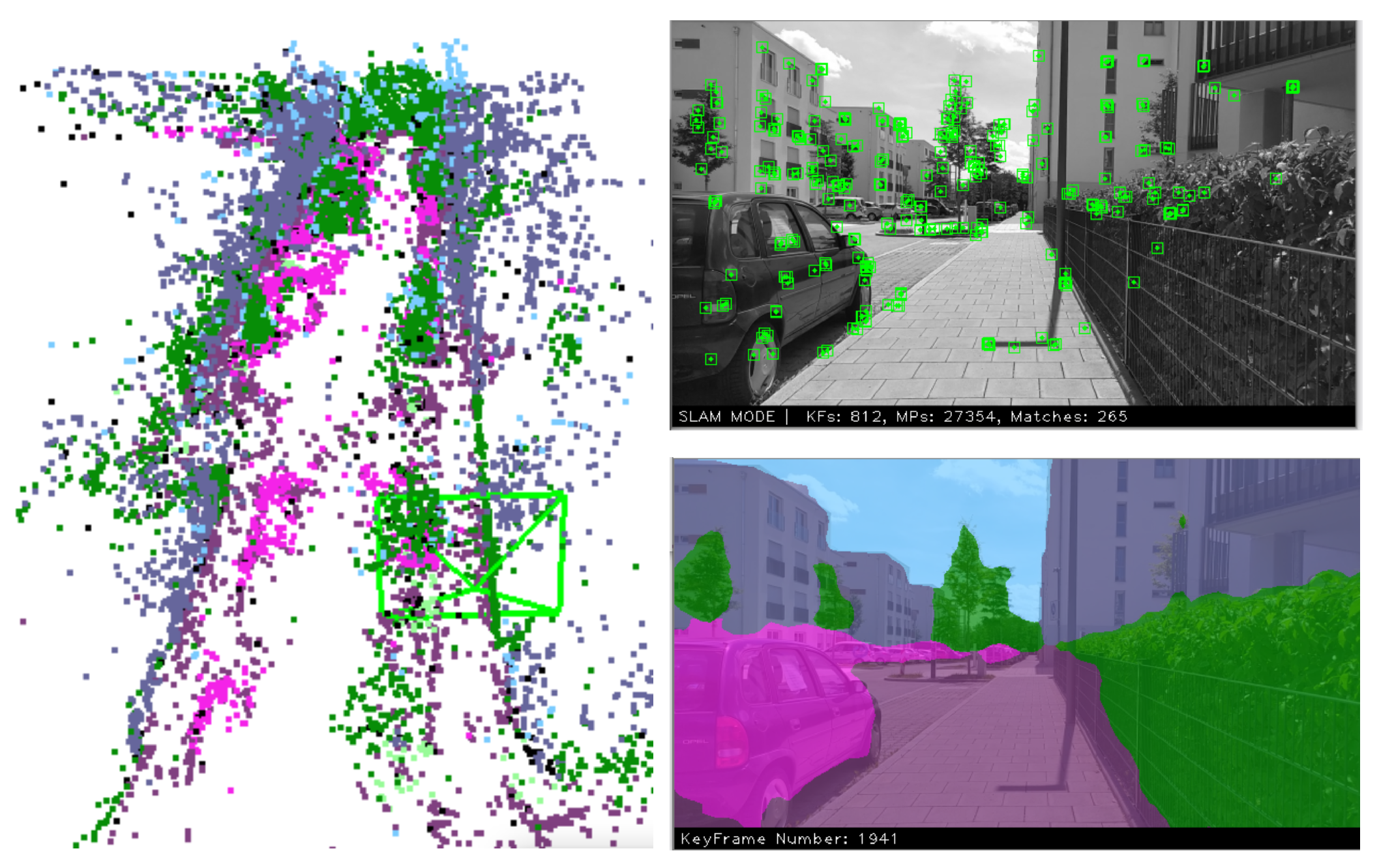
3.1. ORB-SLAM2
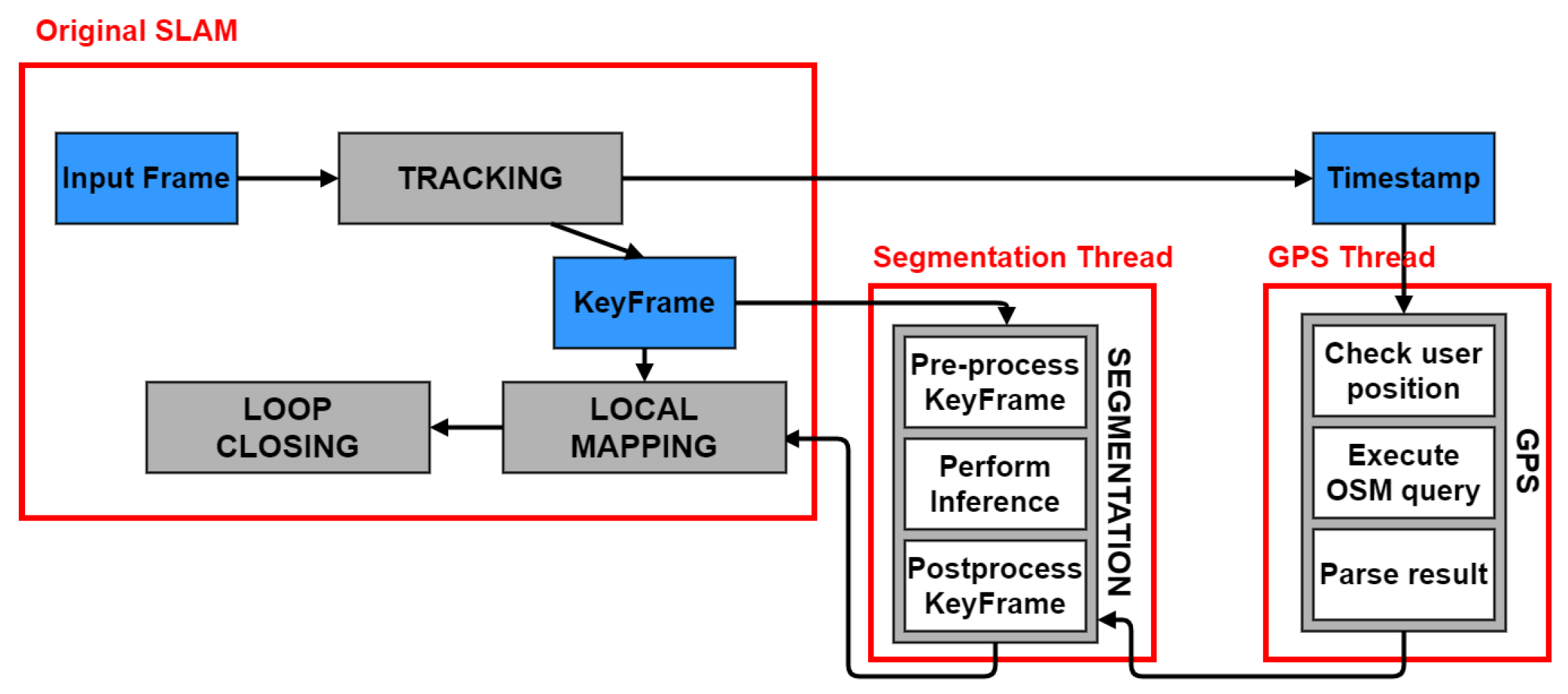
- Tracking: it computes the camera pose for every new frame, based on feature matching and bundle adjustment. It also takes care of relocalization and selects new keyframes.
- Local Mapping: it receives the keyframes and inserts new 3D points in the map. It also optimizes the local map.
- Loop Closing: it uses the last processed keyframe to search for loops. If one is detected, the accumulated drift is computed and the map is corrected.
3.2. Fast-SCNN
4. Implementation
4.1. Fusion of SLAM and Neural Network
- Minimize the number of neural network inferences.
- Minimize the idle time of a thread waiting for the segmentation result.
- Label Fusion: Even though a complete label fusion method is not present, we exploited the knowledge of the points’ probability to reduce the number of unlabeled points and increase the probability of the labeled ones. In fact, when duplicated points are fused by the local mapping or loop closure threads, we keep the class corresponding to the highest probability between the two.
- Frame Skipping: This is a simple way to improve ORB-SLAM2 efficiency. The idea is based on the fact that it is common for an AR user to not move for some time while using the application. In these moments, the frames are similar to one another, so it is not necessary to process them at a high frequency, but some can be skipped, thus saving computations. Therefore, in the tracking thread, at the end of an iteration, the frame’s pose is inspected. If the user has not moved, the next frame is skipped. This is not performed during the initialization or the relocalization.
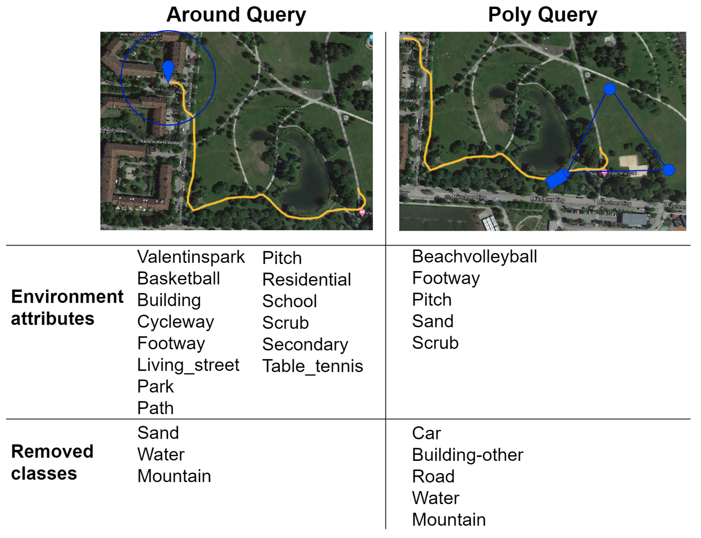
4.2. GPS Integration
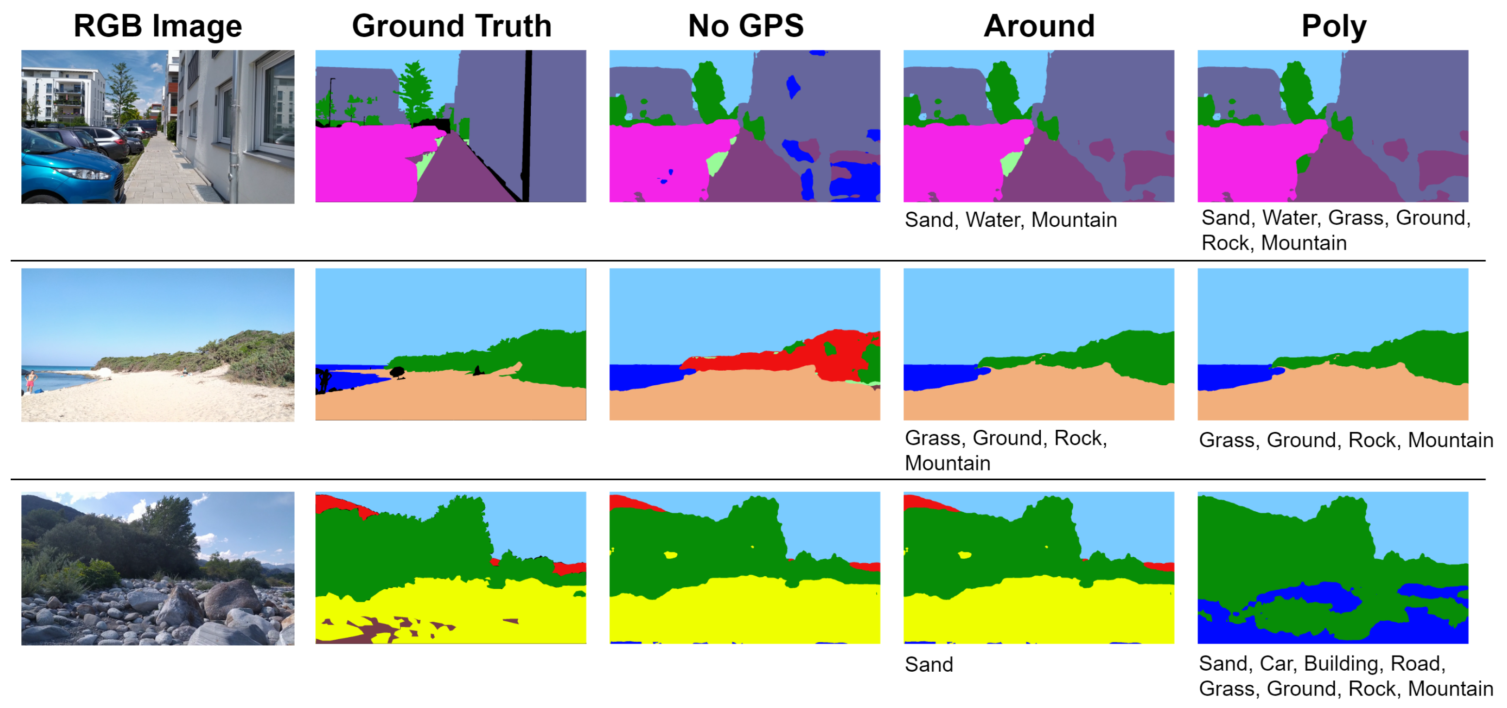
- Circle around the User (around keyword): query for all the elements contained in a circle of fixed radius around the user’s current location.
- Camera Field of View (poly keyword): retrieve only the features that are present in the user’s camera field of view by specifying a triangle representing it.
4.3. Fast-SCNN Training
5. Evaluation
5.1. Datasets
5.2. Fast-SCNN Evaluation
5.3. GPS Integration Evaluation
5.4. EnvSLAM Evaluation
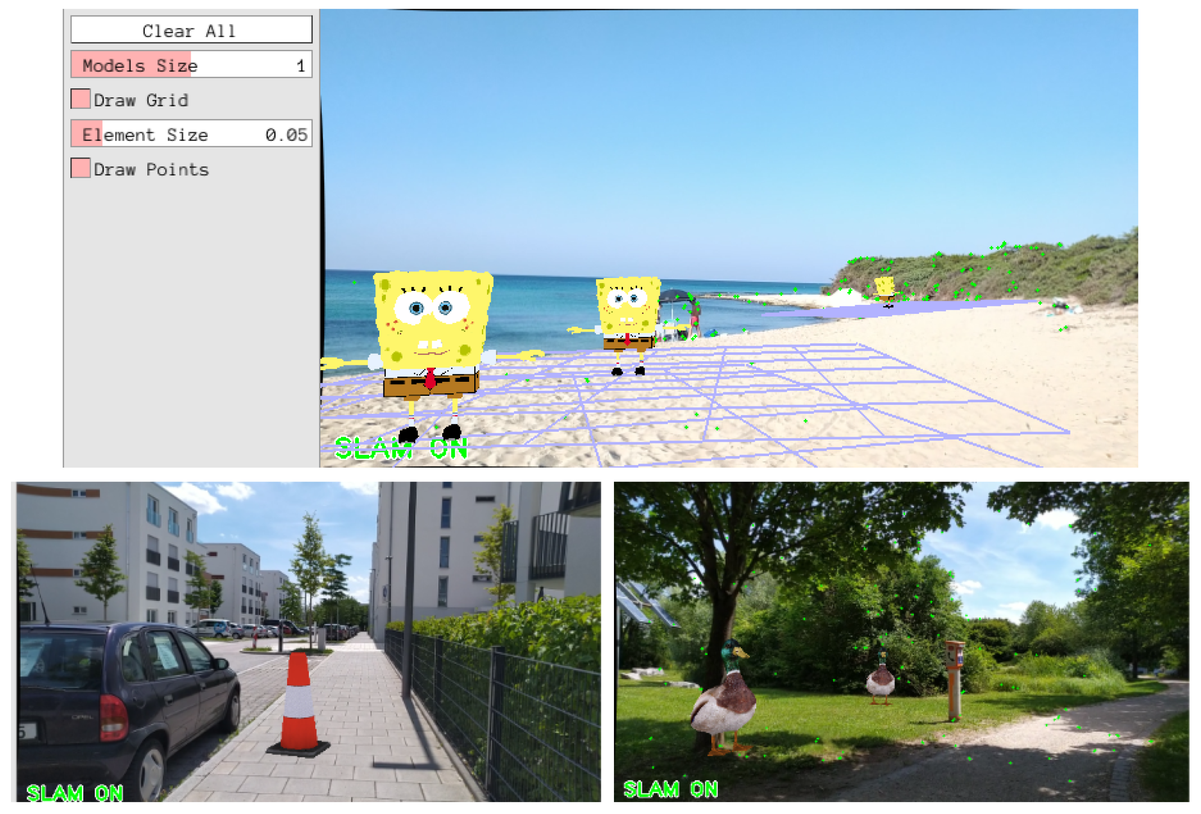
6. Proof of Concept: AR Application
7. Conclusions
8. Future Work
Author Contributions
Funding
Institutional Review Board Statement
Informed Consent Statement
Data Availability Statement
Conflicts of Interest
References
- Azuma, R.T. A Survey of Augmented Reality. Presence Teleoper. Virtual Environ. 1997, 6, 355–385. [Google Scholar] [CrossRef]
- Siltanen, S. Theory and Applications of Marker Based Augmented Reality. Ph.D. Thesis, Aalto University, Espoo, Finland, 2012. [Google Scholar]
- Oufqir, Z.; El Abderrahmani, A.; Satori, K. From Marker to Markerless in Augmented Reality. In Embedded Systems and Artificial Intelligence; Sidi Mohamed Ben Abdellah University: Fez, Morocco, 2020; pp. 599–612. [Google Scholar]
- Reitmayr, G.; Langlotz, T.; Wagner, D.; Mulloni, A.; Schall, G.; Schmalstieg, D.; Pan, Q. Simultaneous Localization and Mapping for Augmented Reality. In Proceedings of the International Symposium on Ubiquitous Virtual Reality, Gwangju, Korea, 13 July 2010; pp. 5–8. [Google Scholar]
- Chatzopoulos, D.; Bermejo, C.; Huang, Z.; Hui, P. Mobile Augmented Reality Survey: From Where We Are to Where We Go. IEEE Access 2017, 5, 6917–6950. [Google Scholar] [CrossRef]
- Meingast, M.; Geyer, C.; Sastry, S. Geometric Models of Rolling-Shutter Cameras. In Proceedings of the Omnidirectional Vision, Camera Networks and Non-Classical Cameras, Kyoto, Japan, 4 October 2009. [Google Scholar]
- Cavallari, T. Semantic Slam: A New Paradigm for Object Recognition and Scene Reconstruction. Ph.D. Thesis, University of Bologna, Bologna, Italy, 2017. [Google Scholar]
- Ülkü, I.; Akagündüz, E. A Survey on Deep Learning-based Architectures for Semantic Segmentation on 2D images. arXiv 2020, arXiv:1912.19230v2. [Google Scholar]
- Xu, J.; Cao, H.; Li, D.; Huang, K.; Qian, C.; Shangguan, L.; Yang, Z. Edge Assisted Mobile Semantic Visual SLAM. In Proceedings of the IEEE Conference on Computer Communications (INFOCOM), Toronto, ON, Canada, 6–9 July 2020; pp. 1828–1837. [Google Scholar]
- Poudel, R.P.K.; Liwicki, S.; Cipolla, R. Fast-SCNN: Fast Semantic Segmentation Network. In Proceedings of the British Machine Vision Conference (BMVC), Aberystwyth, UK, 3 September 2019; p. 289. [Google Scholar]
- Frese, U.; Wagner, R.; Röfer, T. A SLAM Overview from a User’s Perspective. Künstliche Intell. (KI) 2010, 24, 191–198. [Google Scholar] [CrossRef]
- Cadena, C.; Carlone, L.; Carrillo, H.; Latif, Y.; Scaramuzza, D.; Neira, J.; Reid, I.; Leonard, J.J. Past, Present, and Future of Simultaneous Localization and Mapping: Toward the Robust-Perception Age. IEEE Trans. Robot. 2016, 32, 1309–1332. [Google Scholar] [CrossRef] [Green Version]
- Younes, G.; Asmar, D.C.; Shammas, E.A. A survey on non-filter-based monocular Visual SLAM systems. arXiv 2018, arXiv:1607.00470v1. [Google Scholar]
- Younes, G.; Asmar, D.; Shammas, E.; Zelek, J. Keyframe-based monocular SLAM: Design, survey, and future directions. Robot. Auton. Syst. 2017, 98, 67–88. [Google Scholar] [CrossRef] [Green Version]
- Engel, J.; Schöps, T.; Cremers, D. LSD-SLAM: Large-scale direct monocular SLAM. In Proceedings of the Computer Vision—ECCV Proceedings, Part II, Zurich, Switzerland, 6 September 2014; pp. 834–849. [Google Scholar]
- Newcombe, R.A.; Lovegrove, S.J.; Davison, A.J. DTAM: Dense tracking and mapping in real-time. In Proceedings of the 2011 International Conference on Computer Vision, Barcelona, Spain, 13 November 2011; pp. 2320–2327. [Google Scholar]
- Engel, J.; Koltun, V.; Cremers, D. Direct Sparse Odometry. arXiv 2016, arXiv:1607.02565. [Google Scholar] [CrossRef] [PubMed]
- Klein, G.; Murray, D. Parallel Tracking and Mapping for Small AR Workspaces; IEEE: Manhattan, NY, USA, 2007; pp. 225–234. [Google Scholar]
- Herrera, D.; Kim, K.; Kannala, J.; Pulli, K.; Heikkilä, J. DT-SLAM: Deferred triangulation for Robust SLAM. In Proceedings of the International Conference on 3D Vision, Tokyo, Japan, 8 December 2014; Volume 1, pp. 609–616. [Google Scholar]
- Mur-Artal, R.; Tardós, J.D. ORB-SLAM2: An Open-Source SLAM System for Monocular, Stereo, and RGB-D Cameras. IEEE Trans. Robot. 2017, 33, 1255–1262. [Google Scholar] [CrossRef] [Green Version]
- Forster, C.; Zhang, Z.; Gassner, M.; Werlberger, M.; Scaramuzza, D. SVO: Semi-Direct Visual Odometry for Monocular and Multi-Camera Systems. IEEE Trans. Robot. 2017, 33, 249–265. [Google Scholar] [CrossRef] [Green Version]
- Davison, A.J.; Reid, I.D.; Molton, N.D.; Stasse, O. MonoSLAM: Real-Time Single Camera SLAM. IEEE Trans. Pattern Anal. Mach. Intell. 2007, 29, 1052–1067. [Google Scholar] [CrossRef] [Green Version]
- Mur-Artal, R.; Montiel, J.M.M.; Tardós, J.D. ORB-SLAM: A Versatile and Accurate Monocular SLAM System. IEEE Trans. Robot. 2015, 31, 1147–1163. [Google Scholar] [CrossRef] [Green Version]
- Saffar, M.H.; Fayyaz, M.; Sabokrou, M.; Fathy, M. Semantic Video Segmentation: A Review on Recent Approaches. arXiv 2018, arXiv:1806.06172. [Google Scholar]
- Siam, M.; Gamal, M.; Abdel-Razek, M.; Yogamani, S.K.; Jägersand, M. RTSeg: Real-Time Semantic Segmentation Comparative Study. In Proceedings of the 2018 25th IEEE International Conference on Image Processing (ICIP), Athens, Greece, 7–10 October 2018; pp. 1603–1607. [Google Scholar]
- Li, B.; Shi, Y.; Chen, Z. A Survey on Semantic Segmentation. In Proceedings of the 2018 IEEE International Conference on Data Mining Workshops (ICDMW), Singapore, 17–20 November 2018; pp. 1233–1240. [Google Scholar]
- Chen, L.C.; Papandreou, G.; Schroff, F.; Adam, H. Rethinking Atrous Convolution for Semantic Image Segmentation. arXiv 2017, arXiv:1706.05587. [Google Scholar]
- He, K.; Gkioxari, G.; Dollár, P.; Girshick, R.B. Mask R-CNN. IEEE Trans. Pattern Anal. Mach. Intell. 2020, 42, 386–397. [Google Scholar] [CrossRef] [PubMed]
- Lin, T.Y.; Maire, M.; Belongie, S.J.; Hays, J.; Perona, P.; Ramanan, D.; Dollár, P.; Zitnick, C.L. Microsoft COCO: Common Objects in Context. arXiv 2014, arXiv:1405.0312. [Google Scholar]
- Ren, S.; He, K.; Girshick, R.B.; Sun, J. Faster R-CNN: Towards Real-Time Object Detection with Region Proposal Networks. IEEE Trans. Pattern Anal. Mach. Intell. 2017, 39, 1137–1149. [Google Scholar] [CrossRef] [Green Version]
- Han, S.; Mao, H.; Dally, W. Deep Compression: Compressing Deep Neural Network with Pruning, Trained Quantization and Huffman Coding. arXiv 2016, arXiv:1510.00149v5. [Google Scholar]
- Li, H.; Kadav, A.; Durdanovic, I.; Samet, H.; Graf, H. Pruning Filters for Efficient ConvNets. arXiv 2017, arXiv:1608.08710v3. [Google Scholar]
- Poudel, R.P.K.; Bonde, U.; Liwicki, S.; Zach, C. ContextNet: Exploring Context and Detail for Semantic Segmentation in Real-time. In Proceedings of the British Machine Vision Conference (BMVC), Newcastle, UK, 3–6 September 2018; p. 146. [Google Scholar]
- Hubara, I.; Courbariaux, M.; Soudry, D.; El-Yaniv, R.; Bengio, Y. Binarized Neural Networks. In Proceedings of the Advances in Neural Information Processing Systems 29: Annual Conference on Neural Information Processing Systems, Barcelona, Spain, 5 December 2016; pp. 4107–4115. [Google Scholar]
- Rastegari, M.; Ordonez, V.; Redmon, J.; Farhadi, A. XNOR-Net: ImageNet Classification Using Binary Convolutional Neural Networks. In Proceedings of the Computer Vision—ECCV Proceedings, Part IV, Amsterdam, The Netherlands, 11–14 October 2016; pp. 525–542. [Google Scholar]
- Wu, S.; Li, G.; Chen, F.; Shi, L. Training and Inference with Integers in Deep Neural Networks. In Proceedings of the International Conference on Learning Representations, Vancouver, BC, Canada, 30 April 2018. [Google Scholar]
- Li, X.; Zhou, Y.; Pan, Z.; Feng, J. Partial Order Pruning: For Best Speed/Accuracy Trade-Off in Neural Architecture Search. In Proceedings of the 2019 IEEE/CVF Conference on Computer Vision and Pattern Recognition (CVPR), Long Beach, CA, USA, 15–20 June 2019; pp. 9145–9153. [Google Scholar]
- Wang, Y.; Zhou, Q.; Liu, J.; Xiong, J.; Gao, G.; Wu, X.; Latecki, L.J. LEDNet: A Lightweight Encoder-Decoder Network for Real-Time Semantic Segmentation. In Proceedings of the IEEE International Conference on Image Processing (ICIP), Taipei, Taiwan, 22–25 September 2019; pp. 1860–1864. [Google Scholar]
- Howard, A.; Sandler, M.; Chu, G.; Chen, L.C.; Chen, B.; Tan, M.; Wang, W.; Zhu, Y.; Pang, R.; Vasudevan, V.; et al. Searching for MobileNetV3. In Proceedings of the IEEE/CVF International Conference on Computer Vision (ICCV), Seoul, Korea, 27 October–2 November 2019; pp. 1314–1324. [Google Scholar]
- Chao, P.; Kao, C.Y.; Ruan, Y.S.; Huang, C.H.; Lin, Y.L. HarDNet: A Low Memory Traffic Network. In Proceedings of the IEEE/CVF International Conference on Computer Vision (ICCV), Seoul, Korea, 27 October–2 November 2019; pp. 3551–3560. [Google Scholar]
- Li, R.; Wang, S.; Gu, D. Ongoing Evolution of Visual SLAM from Geometry to Deep Learning: Challenges and Opportunities. Cogn. Comput. 2018, 10, 875–889. [Google Scholar] [CrossRef]
- Tateno, K.; Tombari, F.; Laina, I.; Navab, N. CNN-SLAM: Real-Time Dense Monocular SLAM with Learned Depth Prediction. In Proceedings of the IEEE Conference on Computer Vision and Pattern Recognition (CVPR), Honolulu, HI, USA, 21 July 2017; pp. 6565–6574. [Google Scholar]
- Costante, G.; Mancini, M.; Valigi, P.; Ciarfuglia, T.A. Exploring Representation Learning With CNNs for Frame-to-Frame Ego-Motion Estimation. IEEE Robot. Autom. Lett. 2016, 1, 18–25. [Google Scholar] [CrossRef]
- DeTone, D.; Malisiewicz, T.; Rabinovich, A. Toward Geometric Deep SLAM. arXiv 2017, arXiv:1707.07410. [Google Scholar]
- Bao, S.Y.; Bagra, M.; Chao, Y.; Savarese, S. Semantic Structure From Motion with Points, Regions, and Objects. In Proceedings of the IEEE Conference on Computer Vision and Pattern Recognition, Providence, RI, USA, 16–21 June 2012; pp. 2703–2710. [Google Scholar]
- Rosinol, A.; Gupta, A.; Abate, M.; Shi, J.; Carlone, L. 3d dynamic scene graphs: Actionable spatial perception with places, objects, and humans. arXiv 2020, arXiv:2002.06289. [Google Scholar]
- Yu, C.; Liu, Z.; Liu, X.; Xie, F.; Yang, Y.; Wei, Q.; Qiao, F. DS-SLAM: A Semantic Visual SLAM towards Dynamic Environments. In Proceedings of the IEEE/RSJ International Conference on Intelligent Robots and Systems (IROS), Madrid, Spain, 1–5 October 2018; pp. 1168–1174. [Google Scholar]
- Zhong, F.; Wang, S.; Zhang, Z.; Chen, C.; Wang, Y. Detect-SLAM: Making Object Detection and SLAM Mutually Beneficial. In Proceedings of the IEEE Winter Conference on Applications of Computer Vision (WACV), Lake Tahoe, NV, USA, 12–15 March 2018; pp. 1001–1010. [Google Scholar]
- Salas-Moreno, R.F.; Newcombe, R.A.; Strasdat, H.; Kelly, P.H.J.; Davison, A.J. SLAM++: Simultaneous Localisation and Mapping at the Level of Objects. In Proceedings of the IEEE Conference on Computer Vision and Pattern Recognition, Portland, Oregon, USA, 13–18 June 2013; pp. 1352–1359. [Google Scholar]
- McCormac, J.; Clark, R.; Bloesch, M.; Davison, A.J.; Leutenegger, S. Fusion++: Volumetric Object-Level SLAM. In Proceedings of the International Conference on 3D Vision (3DV), Verona, Italy, 5–8 September 2018; pp. 32–41. [Google Scholar]
- Rünz, M.; Agapito, L. MaskFusion: Real-Time Recognition, Tracking and Reconstruction of Multiple Moving Objects. In Proceedings of the IEEE International Symposium on Mixed and Augmented Reality (ISMAR), Munich, Germany, 16–20 October 2018; pp. 10–20. [Google Scholar]
- Hachiuma, R.; Pirchheim, C.; Schmalstieg, D.; Saito, H. DetectFusion: Detecting and Segmenting Both Known and Unknown Dynamic Objects in Real-time SLAM. arXiv 2019, arXiv:1907.09127. [Google Scholar]
- Zhao, Z.; Mao, Y.J.; Ding, Y.; Ren, P.; Zheng, N.N. Visual-Based Semantic SLAM with Landmarks for Large-Scale Outdoor Environment. In Proceedings of the China Symposium on Cognitive Computing and Hybrid Intelligence (CCHI), Xi’an, China, 21–22 September 2019; pp. 149–154. [Google Scholar]
- Tateno, K.; Tombari, F.; Navab, N. Real-time and scalable incremental segmentation on dense SLAM. In Proceedings of the IEEE/RSJ International Conference on Intelligent Robots and Systems (IROS), Hamburg, Germany, 28 September–2 October 2015; pp. 4465–4472. [Google Scholar]
- Zhao, H.; Shi, J.; Qi, X.; Wang, X.; Jia, J. Pyramid Scene Parsing Network. In Proceedings of the IEEE Conference on Computer Vision and Pattern Recognition (CVPR), Honolulu, HI, USA, 21–26 July 2017; pp. 6230–6239. [Google Scholar]
- McCormac, J.; Handa, A.; Davison, A.J.; Leutenegger, S. SemanticFusion: Dense 3D semantic mapping with convolutional neural networks. In Proceedings of the IEEE International Conference on Robotics and Automation (ICRA), Singapore, 29 May–3 June 2017; pp. 4628–4635. [Google Scholar]
- Nakajima, Y.; Tateno, K.; Tombari, F.; Saito, H. Fast and Accurate Semantic Mapping through Geometric-based Incremental Segmentation. In Proceedings of the IEEE/RSJ International Conference on Intelligent Robots and Systems (IROS), Madrid, Spain, 1–5 October 2018; pp. 385–392. [Google Scholar]
- Li, X.; Belaroussi, R. Semi-Dense 3D Semantic Mapping from Monocular SLAM. arXiv 2016, arXiv:1611.04144. [Google Scholar]
- Kiss-Illés, D.; Barrado, C.; Salamí, E. GPS-SLAM: An augmentation of the ORB-SLAM algorithm. Sensors 2019, 19, 4973. [Google Scholar] [CrossRef] [PubMed] [Green Version]
- Ardeshir, S.; Collins-Sibley, K.M.; Shah, M. Geo-Semantic Segmentation. In Proceedings of the IEEE Conference on Computer Vision and Pattern Recognition (CVPR), Boston, MA, USA, 7–12 June 2015; pp. 2792–2799. [Google Scholar]
- Hosseinyalamdary, S.; Balazadegan, Y.; Toth, C. Tracking 3D Moving Objects Based on GPS/IMU Navigation Solution, Laser Scanner Point Cloud and GIS Data. ISPRS Int. J. Geo-Inf. 2015, 4, 1301–1316. [Google Scholar] [CrossRef]
- Ardeshir, S.; Zamir, A.; Torroella, A.; Shah, M. GIS-Assisted Object Detection and Geospatial Localization; Computer Vision: Zurich, Switzerland, 2014; pp. 602–617. [Google Scholar]
- Zhao, H.; Qi, X.; Shen, X.; Shi, J.; Jia, J. ICNet for Real-Time Semantic Segmentation on High-Resolution Images. In Proceedings of the Computer Vision—ECCV Proceecings, Part III, Munich, Germany, 8–14 September 2018; pp. 418–434. [Google Scholar]
- Caesar, H.; Uijlings, J.R.R.; Ferrari, V. COCO-Stuff: Thing and Stuff Classes in Context. In Proceedings of the IEEE/CVF Conference on Computer Vision and Pattern Recognition, Salt Lake City, UT, USA, 18–23 June 2018; pp. 1209–1218. [Google Scholar]
- Cordts, M.; Omran, M.; Ramos, S.; Rehfeld, T.; Enzweiler, M.; Benenson, R.; Franke, U.; Roth, S.; Schiele, B. The Cityscapes Dataset for Semantic Urban Scene Understanding. In Proceedings of the IEEE Conference on Computer Vision and Pattern Recognition (CVPR), Las Vegas, NV, USA, 27–30 June 2016; pp. 3213–3223. [Google Scholar]
- Blanco, J.L.; Moreno, F.; González-Jiménez, J. The Málaga urban dataset: High-rate stereo and LiDAR in a realistic urban scenario. Int. J. Robot. Res. 2014, 33, 207–214. [Google Scholar] [CrossRef] [Green Version]
- Shrivastava, A.; Gupta, A.; Girshick, R.B. Training Region-Based Object Detectors with Online Hard Example Mining. In Proceedings of the IEEE Conference on Computer Vision and Pattern Recognition (CVPR), Las Vegas, NV, USA, 27–30 June 2016; pp. 761–769. [Google Scholar]
- Eichhorn, C.; Jadid, A.; Plecher, D.A.; Weber, S.; Klinker, G.; Itoh, Y. Catching the Drone-A Tangible Augmented Reality Game in Superhuman Sports. In Proceedings of the IEEE International Symposium on Mixed and Augmented Reality Adjunct (ISMAR-Adjunct), Recife, Brazil, 9–13 November 2020; pp. 24–29. [Google Scholar]
- Vlahakis, V.; Ioannidis, M.; Karigiannis, J.; Tsotros, M.; Gounaris, M.; Stricker, D.; Gleue, T.; Daehne, P.; Almeida, L. Archeoguide: An augmented reality guide for archaeological sites. IEEE Comput. Graph. Appl. 2002, 22, 52–60. [Google Scholar] [CrossRef]
- Plecher, D.A.; Wandinger, M.; Klinker, G. Mixed Reality for Cultural Heritage. In Proceedings of the IEEE Conference on Virtual Reality and 3D User Interfaces (VR), Osaka, Japan, 23–27 March 2019; pp. 1618–1622. [Google Scholar]
- Poulose, A.; Han, D. Hybrid Indoor Localization Using IMU Sensors and Smartphone Camera. Sensors 2019, 19, 5084. [Google Scholar] [CrossRef] [PubMed] [Green Version]


| Name | Camera | OA | FPS | Resolution | Map | I | K | L | GPS |
|---|---|---|---|---|---|---|---|---|---|
| SLAM++ [49] | RGB-D | ✓ | 20 fps | / | Dense | ||||
| Fusion++ [50] | RGB-D | ✓ | 4–8 fps | 640 × 480 | Dense | ✓ | |||
| MaskFusion [51] | RGB-D | ✓ | ✓-30 fps if static | 640 × 480 | Dense | ||||
| DetectFusion [52] | RGB-D | ✓ | 22 fps | 640 × 480 | Dense | ||||
| SemanticFusion [56] | RGB-D | 25 fps | 320 × 240 | Dense | ✓ | ✓ | |||
| Nakajima et al. [57] | RGB-D | ✓-30 fps | 40 × 30 | Dense | ✓ | ||||
| CNN-SLAM [42] | Mono | ✓-30 fps | 320 × 240 | Dense | ✓ | ✓ | |||
| EdgeSLAM [9] | Mono | ✓- 30 fps, server | 1280 × 720 | Sparse | ✓ | ✓ | |||
| Li et al. [58] | Mono | 10 fps | 1392 × 521 | Semi-dense | ✓ | ✓ | |||
| Zhao et al. [53] | Mono | 1.8 fps | 1392 × 512 | Sparse | ✓ | ✓ | |||
| EnvSLAM (ours) | Mono | ✓-48 fps | 640 × 360 | Sparse | ✓ | ✓ | ✓ |
| Network | P.A. | Per-Class P.A. | F.W. IoU | Mean IoU | F1 Score | Speed | FLOPs | Params | Size |
|---|---|---|---|---|---|---|---|---|---|
| MobileNetV3 [39] | 52.86% | 26.16% | 34.57% | 17.46% | 25.43% | 19.4 ms | 643.5 | 1.07 M | 12.1 MB |
| Fast-SCNN [10] | 68.52% | 48.25% | 52.55% | 36.96% | 49.91% | 13.9 ms | 329.9 | 1.14 M | 4.73 MB |
| FC-HarDNet [40] | 66.31% | 46.48% | 50.22% | 33.91% | 46.45% | 24.4 ms | 1741.4 | 4.1 M | 16.2 MB |
| DF-Net [37] | 68.26% | 49.41% | 52.51% | 36.39% | 48.87% | 16.0 ms | 3221.7 | 21.1 M | 80.5 MB |
| ICNet [63] | 67.19% | 47.57% | 51.19% | 35.41% | 48.13% | 25.6 ms | 6451.1 | 47.5 M | 181 MB |
| LEDNet [38] | 67.83% | 49.95% | 52.75% | 37.33% | 50.57% | 31.7 ms | 2284.5 | 0.9 M | 60.2 MB |
| Res | P. A. | P.-C. P.A. | F.W. IoU | Mean IoU | F1 Score |
|---|---|---|---|---|---|
| Full | 87.40% | 77.29% | 78.28% | 68.0% | 79.81% |
| Half | 84.48% | 74.30% | 74.0% | 62.92% | 75.92% |
| Case | P. A. | P.-C. P.A. | F.W. IoU | Mean IoU | F1 Score |
|---|---|---|---|---|---|
| No GPS | 89.94% | 73.92% | 82.42% | 65.24% | 74.78% |
| Around | 90.24% | 74.07% | 82.37% | 66.15% | 76.00% |
| Poly | 89.50% | 72.64% | 81.18% | 64.28% | 74.10% |
| System | Full Resolution | Half Resolution |
|---|---|---|
| ORB-SLAM2 | 18.4 fps | 50.2 fps |
| EnvSLAM | 18.2 fps | 48.1 fps |
| Resource | ORB-SLAM2 Full | EnvSLAM Full | ORB-SLAM2 Half | EnvSLAM Half |
|---|---|---|---|---|
| CPU Peak | 69% | 88% | 62% | 63% |
| CPU Average | 43% | 43% | 40% | 42% |
| Start Memory | 594 MB | 2132 MB | 588 MB | 2103 MB |
| End Memory | 1392 MB | 2745 MB | 1604 MB | 2933 MB |
| GPS T. | / | 2.0 s | / | 2.4 s |
| Segmentation T. | / | 53.8 ms | / | 23.8 ms |
Publisher’s Note: MDPI stays neutral with regard to jurisdictional claims in published maps and institutional affiliations. |
© 2021 by the authors. Licensee MDPI, Basel, Switzerland. This article is an open access article distributed under the terms and conditions of the Creative Commons Attribution (CC BY) license (https://creativecommons.org/licenses/by/4.0/).
Share and Cite
Marchesi, G.; Eichhorn, C.; Plecher, D.A.; Itoh, Y.; Klinker, G. EnvSLAM: Combining SLAM Systems and Neural Networks to Improve the Environment Fusion in AR Applications. ISPRS Int. J. Geo-Inf. 2021, 10, 772. https://doi.org/10.3390/ijgi10110772
Marchesi G, Eichhorn C, Plecher DA, Itoh Y, Klinker G. EnvSLAM: Combining SLAM Systems and Neural Networks to Improve the Environment Fusion in AR Applications. ISPRS International Journal of Geo-Information. 2021; 10(11):772. https://doi.org/10.3390/ijgi10110772
Chicago/Turabian StyleMarchesi, Giulia, Christian Eichhorn, David A. Plecher, Yuta Itoh, and Gudrun Klinker. 2021. "EnvSLAM: Combining SLAM Systems and Neural Networks to Improve the Environment Fusion in AR Applications" ISPRS International Journal of Geo-Information 10, no. 11: 772. https://doi.org/10.3390/ijgi10110772
APA StyleMarchesi, G., Eichhorn, C., Plecher, D. A., Itoh, Y., & Klinker, G. (2021). EnvSLAM: Combining SLAM Systems and Neural Networks to Improve the Environment Fusion in AR Applications. ISPRS International Journal of Geo-Information, 10(11), 772. https://doi.org/10.3390/ijgi10110772