FraudMove: Fraud Drivers Discovery Using Real-Time Trajectory Outlier Detection

Abstract

Taxicabs and rideshare cars nowadays are equipped with GPS devices that enable capturing a large volume of traces. These GPS traces represent the moving behavior of the car drivers. Indeed, the real-time discovery of fraud drivers earlier is a demand for saving the passenger’s life and money. For this purpose, this paper proposes a novel time-based system, namely FraudMove, to discover fraud drivers in real-time by identifying outlier active trips. Mainly, the proposed FraudMove system computes the time of the most probable path of a trip. For trajectory outlier detection, a trajectory is considered an outlier trajectory if its time exceeds the time of this computed path by a specified threshold. FraudMove employs a tunable time window parameter to control the number of checks for detecting outlier trips. This parameter allows FraudMove to trade responsiveness with efficiency. Unlike other related works that wait until the end of a trip to indicate that it was an outlier, FraudMove discovers outlier trips instantly during the trip. Extensive experiments conducted on a real dataset confirm the efficiency and effectiveness of FraudMove in detecting outlier trajectories. The experimental results prove that FraudMove saves the response time of the outlier check process by up to 65% compared to the state-of-the-art systems.

1. Introduction

The increasing number of vehicles and taxicabs equipped with GPS can cause a massive volumes of location traces (i.e., trajectories). For example, Uber expanded in over 900 towns across 93 countries with around 103 million monthly average users spread throughout these regions and has up to five million drivers [1]. Detecting outlier trajectories from these massive trajectories can be used in various applications, including transportation management, public safety, and urban planning [2,3,4,5]. Further, distinguishing outlier trajectories from these traces can help in understanding the drivers’ behaviors and traffic conditions [6,7,8,9]. An outlier (or anomaly) trajectory is a trajectory that exhibits different characteristics than normal trajectories [10,11]. Many algorithms were developed to identify outlier trajectories [6,7,12,13]. Most of these algorithms focus on discovering anomalies that have occurred using historical trips [12,13,14]. Despite this, these algorithms suffer from one or more of the following limitations: (a) not applicable for real-time detection of a fraud rideshare driver, (b) low accuracy and high false alarm rate, and (c) outlier trajectory is identified after trip completion.

Detecting outlier trajectories from GPS traces can help in understanding the drivers’ behaviors and traffic conditions [6,7,8,9]. For example, suppose a driver following the suggested route by its rideshare application to deliver his customer. The traffic situation in a real road network changes with time. Consequently, the optimal path within different periods should be different depending on the conditions of the traffic. Suppose that this suggested route has problems such as congested roads and closed roads for emergency conditions (e.g., events, accidents, bad weather, and working area). In this case, the rideshare company does not consider this trip as an outlier trip. In contrast, if the driver takes a different route to deliver the passenger on time, the rideshare company will mark a trip as an outlier ride for that driver. Despite a driver’s current expertise with the route, a ridesharing company regards him as a fraud driver. Hence, distinguishing between true fraud rides and false fraud ones is a need for ridesharing service providers to overcome false alerts and penalties for honest drivers.

This paper proposes a novel real-time trajectory outlier detection system named FraudMove that discovers fraud drivers in an early stage and is based on the trip travel time. This lead to a significant improvement in ridesharing and taxicabs services. The goal of FraudMove is discovering fraud drivers effectively and overcome the following challenges:

• Detect fraud drivers in real-time [7,15]. Efficiently handles the massive GPS data generated by the taxicabs and rideshare cars in a short time.
• Identifying the popular routes that are guaranteed to be both familiar and safe to decide if a trip is an outlier [16]. Extracting the optimal path is a challenge as the definition of optimal varies in different research works. Some studies focus on finding the shortest/fastest path as an optimal path. While in other work, the popular route is the optimal choice if the passenger is not familiar with the area.
• Accurate classification of fraud drivers [6,7]. The traffic conditions change over time. Some drivers may be mislabeled as fraud drivers when taking a different route to deliver the passenger at the time.

The proposed FraudMove system handles the above-mentioned challenges. The major steps of the FraudMove system can be summarized as follows: first, the optimal travel time is computed based on the underlying conditions of the road network for the whole trip from the source S to the destination D. A new version of the Viterbi algorithm [17] is employed to compute the most probable path from historical trips and suggesting it to the user as a recommended optimal path. The outlier trajectory approach is based on the time of this computed optimal path. Next, each time-window, FraudMove checks for delays compared to the previously computed optimal trip time. If the delay time exceeds a predefined threshold, this trajectory is marked as an outlier trajectory and this trip is recognized as a fraud trip for this driver. Finally, FraudMove reports the fraud drivers and differentiates between fraud and honest drivers before finishing the trip and accordingly inform users.

The main contributions of the paper can be summarized as follows:

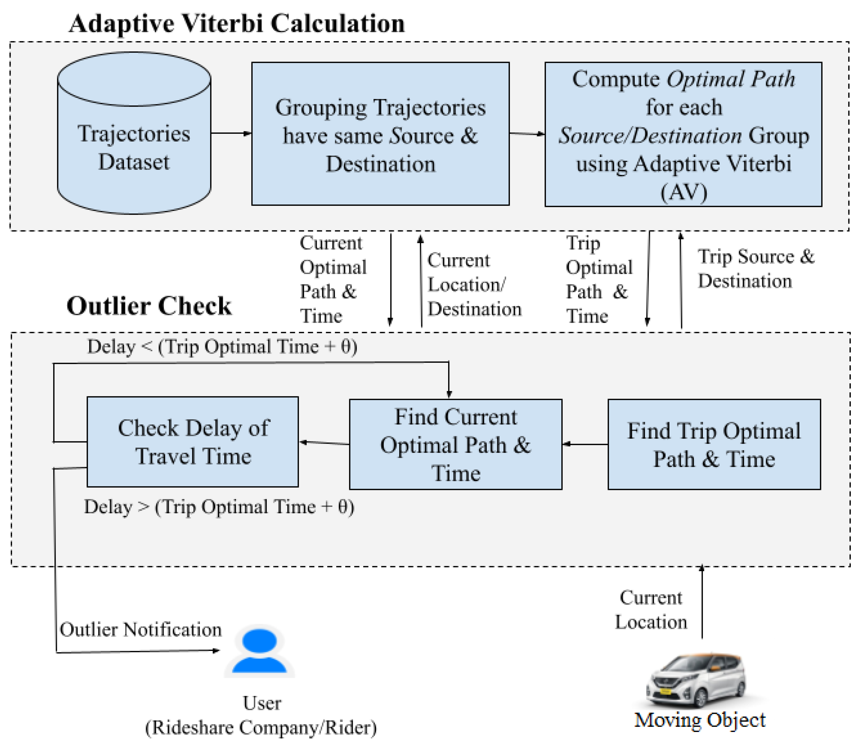
• FraudMove system is proposed for discovering fraud drivers for ongoing trips using a real-time outlier trajectory detection and based on the elapsed trip time.
• An adaptive Viterbi (AV) algorithm is developed to compute the most commonly used route(s) from historical trajectories to be suggested as optimal path(s).
• A novel time-window method is devised to save the computations overhead and minimize the number of needed checks to detect outlier trajectories.
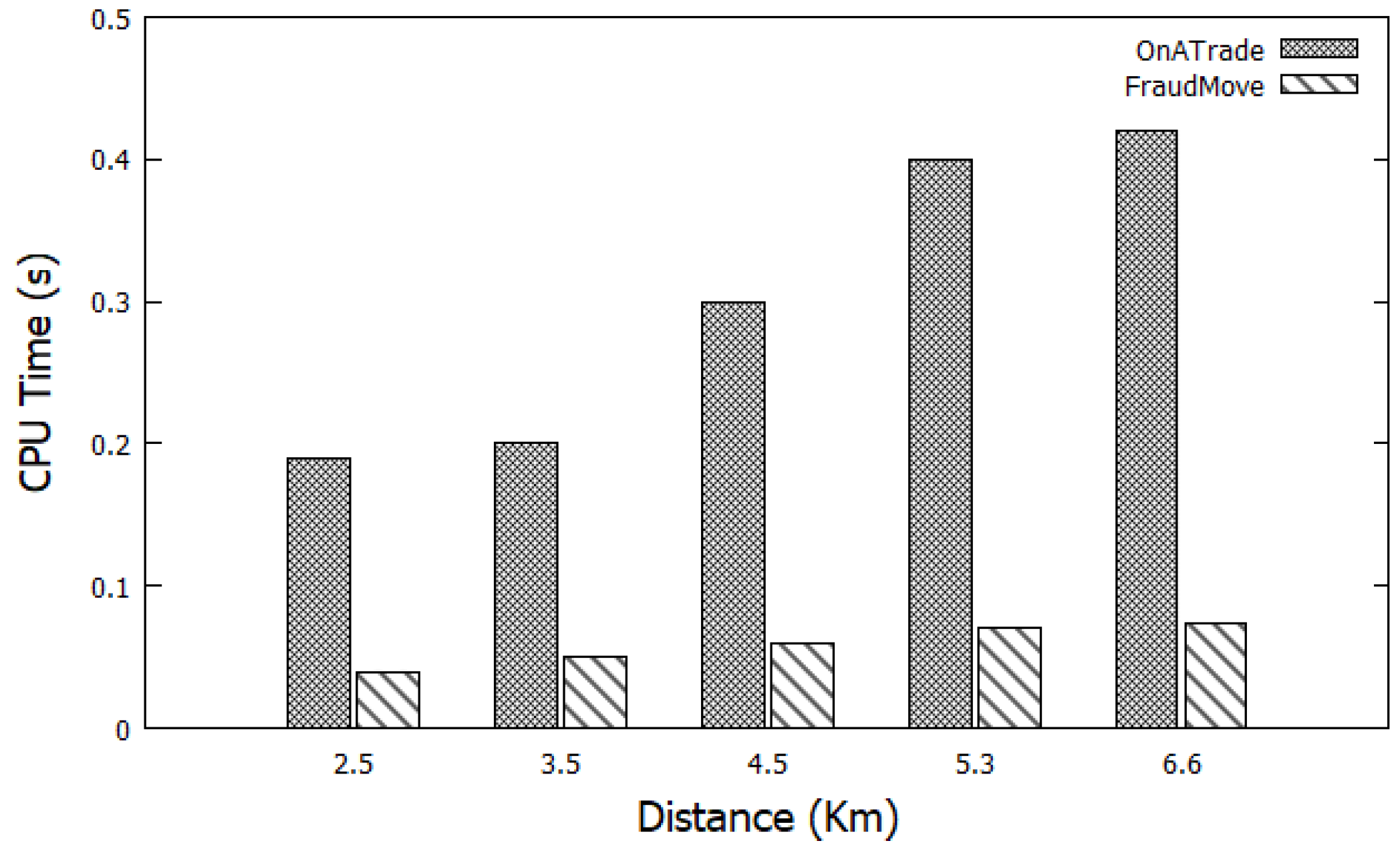
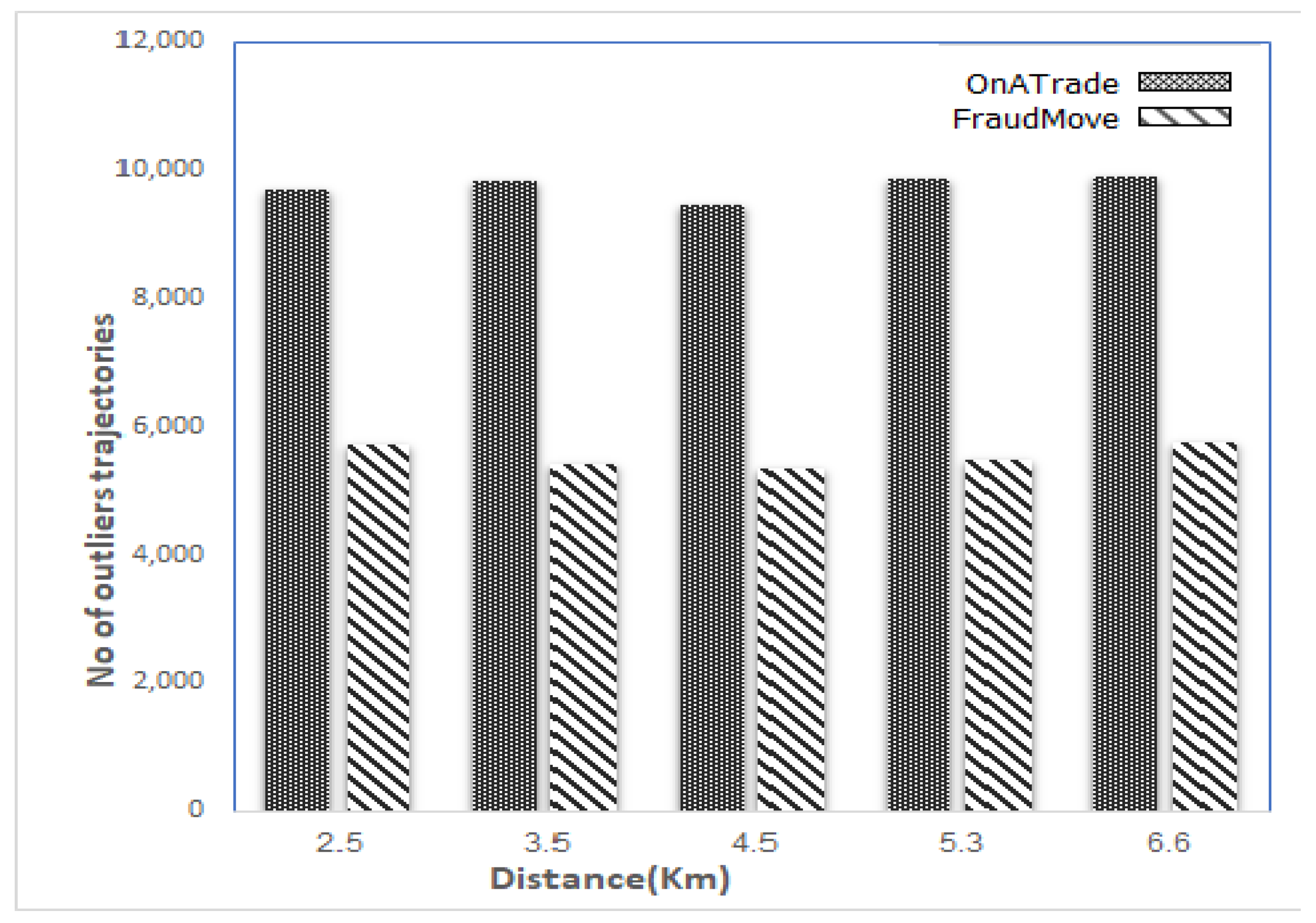
• Intensive experimental evaluations are conducted to ensure the accuracy and efficiency of FraudMove using a real dataset for taxicabs trips in San Francisco, CA, USA. The experimental results confirm that FraudMove outperforms saving in response time by up to 65% compared to the state-of-the-art systems in this direction.

The rest of this paper is organized as follows. Section 2 presents an overview of related work. Section 3 describes preliminary knowledge and problem definition. The proposed solution is presented in Section 4. Section 5 presents our experimental results. Section 6 highlights the significance of our system. Finally, Section 7 concludes the paper.

2. Related Work

In this section, a set of the previous studies are discussed. Previous research related to this paper can be divided into two main directions. The first one focuses on trajectory outlier detection, while the second focuses on mining popular route.

2.1. Trajectory Outlier Detection

The previous studies on trajectory outlier detection can be specifically divided into two main directions: offline trajectory outlier detection algorithms and online (real-time) trajectory outlier detection algorithms.

2.1.1. Offline Trajectory Outlier Detection Algorithms

Most of the previous work in trajectory outlier detection rely on using a historical trajectory dataset to identify outlier trajectories [12,13,14,18]. Distance and density-based outlier detection algorithms are widely used to address a distance or density abnormality in trajectories [14,18,19]. Lee et al. [14] proposed a partition-and-detect framework TRAOD. TRAOD is considered the first algorithm to detect sub-trajectory outliers. TRAOD consists of two phases: (a) partitioning phase, where TRAOD partitions each trajectory into a set of line segments, and (b) detection phase, where density and distance-based measures are used to discover outlying sub-trajectories. A density-based trajectory outlier algorithm called (DBTOD) was suggested by Liu et al. [18]. DBTOD utilizes a density-based approach to detect outliers and classify outliers when a trajectory is local and dense. Ge et al. [19] developed a trajectory outlier detection technique called TOP-EYE algorithm. TOP-EYE employs a decay function to rapidly discover outlier moving trajectories. This approach computes an outlier score cumulatively. Ge et al. [20] have also established a taxi driving fraud detection approach that relies on Dempster–Shafer’s theory and consolidates two pieces of evidence: travel route and proof of driving distance. Moreover, a routemark is used to represent a driving route from an attractive place to another. They use a generative mathematical model based on the routemark to describe the driving distance distribution and to define the proof of driving distance. Further, Kong et al. [21] proposed a long-term traffic anomaly detection (LoTAD) approach. The LoTAD approach is mainly composed of three stages. The first stage constructs a spatial and temporal segment database using the bus trajectory database and the bus station line database. The second step estimates the anomaly index for each path section. Then, using the LOF algorithm [22], they calculated the LOF (local outlier factor) value of each path segment based on the density values. The third stage applies the K-means algorithm on the bus station database for obtaining regions where each cluster represents a region. Next, anomaly scores are defined for each region. Then, those anomalies scores are ordered in decreasing order. Eldawy et al. [23] proposed another method called the clustering-based trajectory outlier detection algorithm (CB-TOD). In the CB-TOD algorithm, the authors summarized the partitions of a trajectory to the smallest set of partitions without affecting the length of the original trajectory. The CB-TOD algorithm used a clustering technique to detect outlier sub-trajectory and also outlier trajectory from the trajectory dataset. Some studies used a pattern model to identify outliers [12,13]. Zhang et al. [12] proposed the iBAT algorithm, which uses the isolation mechanism [24] to discover outlier trajectories. The isolation forest (iForest) function is modified by the iBAT algorithm to isolate outliers’ trajectories from normal ones. Furthermore, they detect outliers’ trajectories based on a few in number and distinguishable from the majority. The TPRO algorithm proposed in [13] also focuses on detecting vehicle trajectory outliers by discovering the most familiar trajectories in each duration for each SD-pair and defining the outlier scores based on the time-dependent edit distances between the query trajectory path and regular trajectories. Nevertheless, the primary limitation of those previous research is that they are not suitable for online detection of outlier trajectories because of their computational overhead.

2.1.2. Online Trajectory Outlier Detection Algorithms

Few algorithms have been proposed for the online study of outlier trajectories [6,7,15]. Daqing Zhang et al. [7] proposed iBOAT algorithm as an upgrade version of the iBAT algorithm [12] to discover outliers trajectories in real time. Further, the iBOAT algorithm is used to discover, which part(s) of a trajectory is an outlier. The authors in [6] proposed the TPRRO algorithm, which is based on the TPRO algorithm, as a real-time outlier detection algorithm to detect trajectories that are not in the historical trajectory dataset. The OnATrade algorithm for optimizing taxi services on GPS big data was developed by Zhou et al. [15]. There are two main phases for OnATrade: path recommendation and online identification. Firstly, it deploys a path recommendation algorithm to generate candidate routes. Secondly, taxis that have irregularities in driving and deviate from the proposed route are recognized. The main shortcomings of this method are that it considered outlier trajectory based on a normal route, sometimes this common route requires extra trip time than other routes based on the changing circumstances of the road. Further, OnATrade retrieves the outlier trajectory after completing the trip. Furthermore, the authors used a labeled dataset, which is impractical for real-time applications.

2.2. Mining Popular Route

Discovering the most popular route has attracted the attention of many researchers and applications. The majority of studies have focused on finding the shortest/fastest path [25,26,27]; however, the most popular route is not necessarily the shortest or fastest. Zaiben et al. [16] proposed a transfer probability network to find a popular route by analyzing historical trajectories. They used historical trajectories to calculate the probability of moving from a specific location to the destination. Further, the transfer probability is used as a popularity measure. The product of the transition probabilities of all important locations on the route determined the route’s popularity. Luo et al. [28] built a network graph, called a footmark graph, to mine frequent paths. They defined the edge frequency as the total number of trajectories moving through the edge. Then, they created a descending edge frequency sequence to determine which direction is the most frequent. The Viterbi algorithm (VA) is a decoder with maximum likelihood. The VA algorithm was first proposed in 1967 by Andrew J. Viterbi [17] for convolutional codes. The VA is a dynamic programming algorithm for discovering the most probable order of hidden states, known as a Viterbi path, that results in a sequence of observed events. It recursively calculates an optimal (i.e., probability-maximizing) state sequence from optimal solutions for sub-problems. It is used usually in the problem of hidden Markov models (HMMs) [29].

The proposed approach FraudMove is different from the previous studies and aims to solve some of the existing limitations. FraudMove is capable of discovering outlier trajectories at an early stage while the rideshare car is still moving and without using a labeled dataset. Moreover, trajectory outlier detection is performed in real time and based on the trip time. A new version of the Viterbi algorithm is proposed to obtain the most probable path from the historical rideshare trips. Finally, a time-window is used to minimize the number of checks to discover fraud drivers.

3. Preliminaries and Problem Definition

This section reviews the preliminaries that are used in the rest of the paper and formalizes the problem statement.

3.1. Preliminaries

In this subsection, we define some of the main concepts that are used in the paper.

Definition 1.

A trajectory τ is a sequence of location points (for example GPS traces) such that $\tau =\{p_1,p_2,p_3,\dots ,p_n\}.$ Each point $p_i$ is represented by $<lo{c}_i,t_i>$ where $lo{c}_i$ is the 2-dimensional geographical coordinates (Latitude, Longitude) of the GPS point $p_i$ at the timestamp $t_i.$

It is difficult to obtain a common path from discrete sampling points of raw trajectories. So in this paper, a preprocessing step is performed on the dataset to map each raw trajectory into the road network and obtain a mapped trajectory ${\tau }_{map}$.

Definition 2.

A road network graph G (V, E, W) is a directed graph, where V is the set of vertices that represents road intersections, E is a set of road edges between vertices, and W is a set of edges weights. $w\in W$ represents the travel time cost of the edge $e_i$.

Definition 3.

A mapped trajectory ${\tau }_{map}$ is a sequence of visited edges for the trajectory τ. Each GPS point is mapped to the corresponding edge in the road network graph G, i.e., ${\tau }_{map}$$=\{E_1,E_2,\dots \dots ,E_m\}$, where m is the number of edges.

Definition 4.

The optimal path OP is the best path depends on the road preferences Pref, where the value of Pref is 0 or 1. The shortest path from the source S to the destination D used when Pref equal to 0; while a most likely route from S to D used at Pref equals 1, as in the following equation:

$$\mathit{Pref}\left(\mathit{x}\right)=\left\{\begin{array}{cc}x=0,\hfill & shortestpathfromStoD\hfill \\ x=1,\hfill & mostlikelypathfromStoD\hfill \end{array}\right.$$

Figure 1 shows an example on the road network graph from the source vertex A to a destination vertex M. The shortest path is marked in red arrows as shown in Figure 1 and contains the following vertices (A, B, E, I, K, M) with a total travel time 14. In this example, the weights on the edges represent the travel time from one node to the next node; thus this path represents the fastest path.

Definition 5.

The optimal time $OT$ is the total travel time along the optimal path OP and is estimated as the sum of edges’ weights along the optimal path (where c represents the number of edges in the OP).

$OT$=${\sum }_{i=0}^c{w}_i\left(E_i\right)$

Definition 6.(Outlier trajectory). Given a Source S and a Destination D of a trajectory τ, the optimal path OP, optimal time $OT$, and the moving object’s current location $CL$, an outlier trajectory is a path that takes a longer travel time than the estimated $OT$ by a given threshold θ.

Definition 7.(Viterbi path). Given a sequence of observations O, the Viterbi path for a given state j at time t was computed as:

$$V_t\left(j\right)=ma{x}_{i=1}^M{V}_{t-1}\left(i\right)a_{ij}{b}_j\left(o_t\right)$$

(1)

$$B{P}_t\left(j\right)=argma{x}_{i=1}^M{V}_{t-1}\left(i\right)a_{ij}{b}_j\left(o_t\right)$$

(2)

where $V_{t-1}\left(i\right)$ is the previous Viterbi path probability from the previous time step. The $a_{ij}$ represents the transition probability from previous state i to current state j, and it is computed as as follows:

$$a_{ij}=\frac{numberoftransitionsfromstateitostatej}{expectednumberoftransitionsfromstatei}$$

(3)

$b_j\left(o_t\right)$ is the state observation likelihood of the observation symbol $\left(o_t\right)$ given the current state j, and it is computed as as follows:

$$b_j\left(o_t\right)=\frac{expectednumberoftimesinstatejobservingsymbol{o}_t}{expectednumberoftimesinstatej}$$

(4)

The $B{P}_t\left(j\right)$ represents the back-pointer that stores the sequence S that yields to the highest probability.

3.2. Problem Statement

Given an on-going trajectory $\tau$ of a moving car, a source location S and a destination location D of the current trip, and a road network graph G (V, E, W), the objective is to discover fraud driving behavior by determining whether $\tau$ is an outlier trajectory or not. The goal of this paper is to perform a trajectory outlier detection process while achieving the following characteristics:

• Real-time processing.
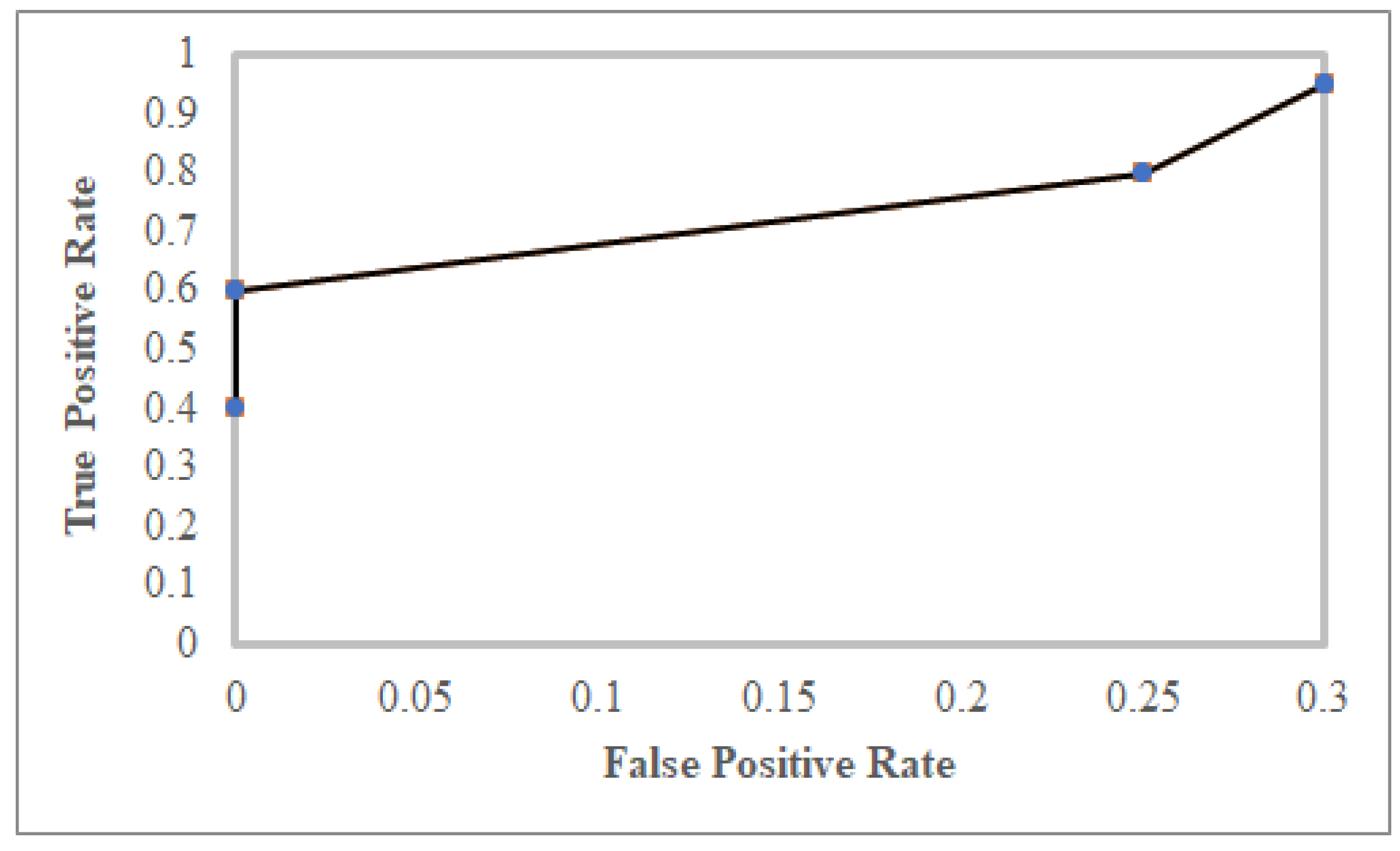
• High classification accuracy.
• Scalability with large numbers of trajectories.

4. FraudMove: Real-Time Trajectory Outlier Detection

This section describes our proposed system FraudMove for detecting outlier trajectories in real-time to discover fraud drivers based on the trip time.

Main idea. The main idea of FraudMove is to compare the travel time cost of the path taken by a driver against the optimal path under the current road conditions. If the driver’s path (consists of the time of the passed part of the trip plus the expected time to reach the final destination) exceeds the optimal path by a predefined time threshold, FraudMove raises an outlier flag. Otherwise, FraudMove would repeat this process periodically along the trip. In other words, the estimated optimal duration of the trip is compared to the actual time of a trip to discover outliers. Then, FraudMove labels this taken path as an outlier path. Consequently, this driver is classified/labeled as a fraud driver.

Figure 2 illustrates the architecture of FraudMove system that consists mainly of two modules: the adaptive Viterbi calculation module and the outlier check module. FraudMove reads the rideshare car’s GPS location and returns an outlier notification if there is an extensive delay from the expected optimal time of a trip. The outlier alarm could be used by rideshare companies and riders to discover any fraud drivers and monitoring rideshare vehicles.

Table 1. List of notations used in this paper.

Symbol	Definition
OP	Optimal path from S to D
OT	Optimal time of the optimal path
$\theta$	Outlier threshold
CL	Current location of a moving object
CP	Optimal path from CL to D
$Trave{l}_T$	Travel time from start to current time
$S{D}_{Trips}$	Trips that share the same S and D
A	Transition matrix
B	Emission matrix
P	Accumulated probability matrix
E	Backtrack matrix

summarizes the list of notations used in this paper and their definition.

4.1. Phase 1: Adaptive Viterbi Calculation

The main purpose of the adaptive Viterbi calculation step in FraudMove is to calculate the optimal path from historical trip data to be used during the outlier check step. This step is an offline step and consists mainly of two phases, namely, Source–Destination (SD) trajectories grouping phase and computing optimal path phase. In the SD trajectories grouping phase, trips that have the same source S and destination D are grouped. Further, the transition matrix A and the emission matrix B [17] are computed for each $S{D}_{Trips}$. In computing the optimal path phase, the most probable path for each $S{D}_{Trips}$ is estimated using the proposed adaptive Viterbi (AV) algorithm. The output path of the AV algorithm is stored in a hash map. The hash map contains the optimal path for each SD pair. In the following subsections, the adaptive Viterbi calculation phases are discussed in detail.

4.1.1. SD Trajectories Grouping

Rideshare cars generate a big trip dataset containing historical GPS raw data of trajectories. The purpose of the SD trajectories grouping phase is gathering trajectories having the same source S and destination D in one single dataset ($S{D}_{Trips}$). This set of GPS traces are converted into a sequence of vertices that match each GPS point to the nearest node on the road network graph G to obtain a mapped trajectory ${\tau }_{map}$. In this paper, when modeling the road network and the spatial environment, the GPS raw data were filtered using digital map modeling [30]. Further, OpenStreetMap(OSM) [31] is used for modeling a digital map of the road network. At the end of this phase, the big trips dataset is divided into small $S{D}_{Trips}$ datasets.

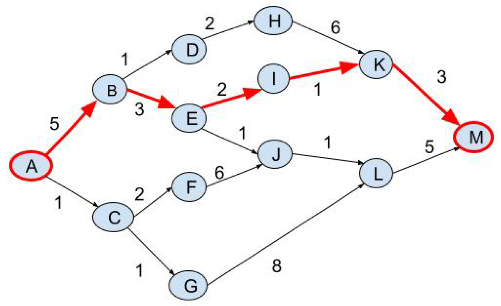
4.1.2. Computing the Optimal Path

The objective of this phase is to determine, using the adaptive Viterbi (AV) algorithm, the optimal path for each $S{D}_{Trips}$ group. The output of this phase is a hash map that stores for each SD pair the optimal path. This optimal path is required for the trajectory outlier detection phase. In this phase, a Viterbi algorithm is adjusted for computing the most probable path from the historical trip data. Then, it is recommended to the driver as an optimal path. The time of this path is used to discover the outlier path.

In this paper, the Viterbi algorithm is adapted to compute the most probable path in $S{D}_{Trips}$ data, the new version is the adaptive Viterbi (AV) algorithm. To provide the characteristics of the trajectory dataset, the adaptive Viterbi (AV) algorithm is adjusted and defined its parameters. In the AV algorithm, the nodes in the path are considered as the hidden states. Further, observations are the ordering of these nodes on the trip. In our computations, the longest trip length (the trip with the maximum number of nodes) is considered as the length of observations. The following are the parameters used in the adaptive Viterbi (AV) algorithm.

• The number of observations M is the length of the longest trip (trip that has the maximum number of nodes) in the $S{D}_{Trips}$.
  M=Length (longest trip ($S{D}_{Trips}$)).
• The transition matrix (A) contains the probability of move from one node (or vertex) to another. It is computed from the historical trip data of the same source S and destination D ($S{D}_{Trips}$). The size of A is N × N, where N is the number of unique nodes in $S{D}_{Trips}$.
• The emission matrix (B) holds the probability of observing a node in a specific order in the path. It is computed from $S{D}_{Trips}$ data and has a size of N × M.
• The Accumulated probability matrix (P). P (n, m) stores the highest probability for a node in a specific order in the route. The matrix P is of size N × M, where $n\in [1:\mathrm{N}]$ and $m\in [1:\mathrm{M}]$. P is recursively calculated using the column index $m\in [1:\mathrm{M}]$.
• The Backtrack matrix (E) stores the indices that yield the highest probability in a matrix P. These indices are required in the step of constructing the most likely path using backtracking. The matrix E is of size N × M − 1.

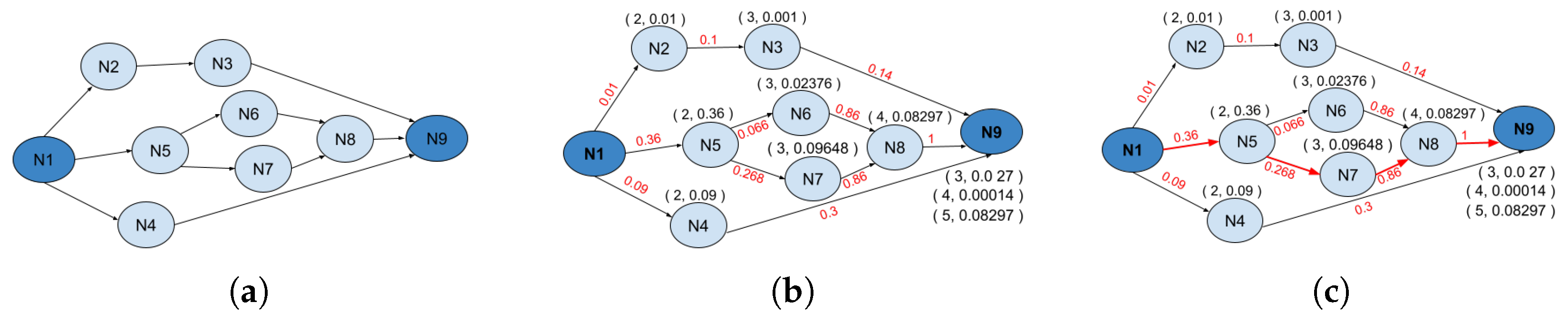
The input for the adaptive Viterbi (AV) algorithm is the source and the destination of the trip, while the output is the best path (most likely path). The initial probability is equal to 1 for the source node of the rideshare trip; as we have no other option except starting from the source node. Details of the AV algorithm are described in the following example.

Example 1.

Suppose to have the rideshare trips data ($S{D}_{Trips}$), as seen in

Table 2. Rideshare trips data.

Trip No	Sequence
$Trip1$	N1 N4 N9
$Trip2$	N1 N5 N6 N8 N9
$Trip3$	N1 N4 N9
$Trip4$	N1 N5 N7 N8 N9
$Trip5$	N1 N5 N6 N8 N9
$Trip6$	N1 N5 N7 N8 N9
$Trip7$	N1 N4 N9
$Trip8$	N1 N2 N3 N9
$Trip9$	N1 N5 N7 N8 N9
$Trip10$	N1 N5 N7 N8 N9

. Such trips reflect going from the same source node (S = N1) to the destination node (D = N9). From this dataset, we build the transition matrix (A) and the emission matrix (B), which are inputs to the AV algorithm. Each cell in the transition matrix stores the probability of departing from one node to the next one in a trip. In

Table 3. Transition matrix (A).

From	To
	N1	N2	N3	N4	N5	N6	N7	N8	N9
N1	0	0.1	0	0.3	0.6	0	0	0	0
N2	0	0	1	0	0	0	0	0	0
N3	0	0	0	0	0	0	0	0	1
N4	0	0	0	0	0	0	0	0	1
N5	0	0	0	0	0	0.33	0.67	0	0
N6	0	0	0	0	0	0	0	1	0
N7	0	0	0	0	0	0	0	1	0
N8	0	0	0	0	0	0	0	0	1
N9	0	0	0	0	0	0	0	0	0

, the transition matrix columns and rows represent the unique nodes in a trajectory dataset. Since the number of different nodes is 9, the transition matrix size is 9 × 9. In an emission matrix, each cell stores the probability of a node in a particular position in the path. In

Table 4. Emission matrix (B).

Node	Order
	1	2	3	4	5
N1	1	0	0	0	0
N2	0	0.1	0	0	0
N3	0	0	0.1	0	0
N4	0	0.3	0	0	0
N5	0	0.6	0	0	0
N6	0	0	0.2	0	0
N7	0	0	0.4	0	0
N8	0	0	0	0.86	0
N9	0	0	0.3	0.14	1

, the emission matrix columns denote the number of transitions in a trip with the maximum trip length in the dataset. Rows represent unique nodes in the $S{D}_{Trips}$. Since the longest route in Table 2 has a length of five and the nodes number is nine; so, the constructed emission matrix is of size 5 × 9.

The following are the details of the computations to retrieve the most probable path. These steps are summarized in

Table 5. Accumulated probability matrix (P).

Node	Probability
	1	2	3	4	5
N1	1	0	0	0	0
N2	0	0.01	0	0	0
N3	0	0	0.001	0	0
N4	0	0.09	0	0	0
N5	0	0.36	0	0	0
N6	0	0	0.02376	0	0
N7	0	0	0.09648	0	0
N8	0	0	0	0.08297	0
N9	0	0	0.027	0.00014	0.08297

with the previous nodes that yield the highest probability each time (as in

Table 6. Backtrack matrix (E).

Node	Order
	1	2	3	4
N1	0	0	0	0
N2	N1	0	0	0
N3	0	N2	0	0
N4	N1	0	0	0
N5	N1	0	0	0
N6	0	N5	0	0
N7	0	N5	0	0
N8	0	0	N7	0
N9	0	N4	N3	N8

).

-

The probability of start from node N1.

P(1, N1) = 1

-

The probability of seeing specific nodes in a second order of the trip. In the given data nodes N2, N4, and N5 are found.

P(2,N2) = P(1,N1)*[P(2|N2)*P(N1,N2)]=1*[0.1*0.1] = 0.01.

P(2,N4) = P(1,N1)*[P(2|N4)*P(N1,N4)]=1*[0.3*0.3] = 0.09.

P(2,N5) = P(1,N1)*[P(2|N5)*P(N1,N5)]=1*[0.6*0.6] = 0.36.

-

The probability of seeing specific nodes in a third order of the trip. In the given data nodes N3, N6, N7, and N9 are found.

P(3,N3) = P(2,N2)*[P(3|N3)*P(N2,N3)] = 0.01*[0.1*1] = 0.001.

P(3,N6) = P(2,N5)*[P(3|N6)*P(N5,N6)] = 0.36*[0.2*0.33] = 0.02376.

P(3,N7) = P(2,N5)*[P(3|N7)*P(N5,N7)] = 0.36*[0.4*0.67] = 0.09648.

P(3,N9) = P(2,N4)*[P(3|N9)*P(N4,N9)] = 0.09*[0.3*1] = 0.027.

-

In the third order of a trip, each node N8 and N9 are found. Node N8 reaches this order given it comes from each of N6 and N7 in the third order in the trip. While node N9 reaches this order given it comes from node N7 in the previous order.

$$P(4,N8)=max\left\{\begin{array}{c}P(3,N6)\ast \left[P\right(4\left|N8\right)\ast P(N6,N8)]=0.02376\ast [0.86\ast 1]=0.02043\hfill \\ P(3,N7)\ast [P\left(4\right|N8)\ast P(N7,N8)]=0.09648\ast [0.86\ast 1]=\underline{0.08297}\hfill \end{array}\right.$$

$$P(4,N9)=P(3,N3)\ast \left[P\right(4\left|N9\right)\ast P(N3,N9)]=0.001\ast [0.14\ast 1]=0.00014$$

In the accumulated probability matrix, the highest probability is stored (0.08297) for seeing a node N8 in order 4 in the trip. Further, in the backtrack matrix, the node that yields this highest probability is stored in the previous order of this node (node N7 as in this stage).

-

In the fifth order of a trip, node N9 only seen. Node N9 reaches to this order given it comes from node N8 in the previous order of it.

P(5,N9) = P(4,N8)*[P(5|N9)*P(N8,N9)] = 0.08297*[1*1] = 0.08297.

In Table 5, the highest probability in each order of a trip is stored in the accumulated matrix P. Table 6 represents the backtrack matrix E and stores the indices that yield to this highest probability. Furthermore, Figure 3a illustrates a sketch of the transition graph that represents the $S{D}_{Trips}$. Moreover, Figure 3b summarizes the previous computations in a transition graph. Finally, Figure 3c shows the best path with a red color where this path is the path with the highest probability. The output is the most likely path (N1 N5 N7 N8 N9) as it has the highest probability (0.08297).

Algorithm. As presented in Algorithm 1, according to the previous example, the adaptive Viterbi algorithm receives as an input (a) the source of the trip S, (b) the destination of the trip D, (c) the transition matrix A, (d) the emission matrix B, (e) the length of observations M, and (f) the length of hidden states N. As output, the algorithm returns the most likely path as the optimal path for these $S{D}_{Trips}$.

The accumulated probability matrix P and backtrack matrix E are initialized to 0 at the start of AV algorithm. As there is no choice except to start from the source node S; so the probability of a node S at order 1 in the accumulated matrix P is fixed to 1. The computations of AV are processed from the second location in the trip to find the most likely node in this order, so the order parameter is initialized to 2. The connected nodes to the source node S are computed using NextNodes HashMap, as in line 10 in Algorithm 1. The NextNodes HashMap is computed from the $S{D}_{Trips}$. It stores a current node as a key and the values are the next nodes to it. The recursion is used to populate the data and filling each of the accumulated probability matrix P and backtrack matrix E, as in line 12 in Algorithm 1. In this step, the AV algorithm iterates to each node that is connected to S and obtains the previous nodes to this node. In the accumulated matrix P, the maximum probability only is stored. Next, in the backtrack matrix E, the node that yields this highest probability from the previous nodes is stored. These steps are repeated after increasing the order by one and obtaining all the nodes that are connected to the nodes in the ConnectedNodes list. The iteration will continue until all the observations in M are examined and filling matrices P and E as illustrated in the previous example. After finishing this step, the backtrack matrix E is used for obtaining the most likely path. From the accumulated probability matrix P, the index of a destination D that has a max probability is obtained (from the previous example N9 in order 5; so, the length of the most probable path is 5). This index is used for constructing the optimal path using backtracking as in line 17 in Algorithm 1.

Algorithm 1 Adaptive Viterbi (AV)
1:	INPUT: Trip source S, Trip destination D, Transition matrix A, Emission matrix B, Observation length M, Hidden states length N.
2:	$\mathbf{SET}P\leftarrow \varphi$
3:	$\mathbf{SET}E\leftarrow \varphi$
4:	$\mathbf{SET}OP\leftarrow \varphi$
5:	/* Set probability of staring from S to 1*/
6:	$\mathbf{SET}P[S,1]\leftarrow 1$
7:	/* Complete from the second location in the trip */
8:	$\mathbf{SET}Order\leftarrow 2$
9:	/* Compute connected nodes to the source S */
10:	$ConnectedNodes$ = Get_Connected_Nodes ((NextNodes, S, Order-1)
11:	/* Recursion to fill matrices P and E */
12:	$Populate\_data$(ConnectedNodes, Loc, A, B, P, E)
13:	/* Backtracking to get optimal path */
14:	$index\leftarrow P\left[D\right].argmax\left(\right)$
15:	/* Using a backtrack matrix E to get OP */
16:	for n = index−1 to 1 do
17:	OP[n] = E [D, n+1]
18:	D = E [D, n+1]
19:	end for
20:	OUTPUT: Return OP

4.2. Phase 2: Outlier Check

In the outlier check phase, checking for outlier trajectories is performed to discover fraud drivers. The user has two options for a preferred route: choose the shortest path from start to destination point or obtained the most likely path. The shortest path option uses the shortest path algorithm [32] to compute it online depending on the current conditions of the road network. In the other option, the most likely path is used, the most likely path is computed using the adaptive Viterbi (AV) algorithm as described in the previous step, as in Algorithm 2 line 2. Further, the time of this path computed from the road network depends on the road conditions. This work claims that the trip travel time is a dynamic factor as it comes through the road network API. The road network API updates itself automatically based on the road conditions. So, the current status of the road is already reflected when we used the road network API to compute trip travel time. So, the actual travel time changes during the travel time estimation.

The outlier trajectory is determined depending on the time factor, so, in this step, the time of the optimal path is computed, that depends on the current conditions of the road network, as in line 8. After starting the trip, and after each time window, the current optimal path is computed depending on the current location, as in Algorithm 2 line 17. A time window parameter is used to decrease the number of checks of outlier detection process (not checks after each update in location). The more frequent the checks, the faster the outlier detection, and the higher the computation cost, and vice versa.

In FraudMove algorithm a static time window S-TW is used, which is a fixed time after firing it an outlier check process is performed. Further, a dynamic time window D-TW is used for enhancing the computations of the FraudMove algorithm. In D-TW, while the ongoing time of a trip is still far away from deviation about the optimal time OT; then FraudMove is skipped the next outlier trajectory check, as in line 21–25 in Algorithm 2.

If (T${}_{CP}$ + Travel${}_T$≤$OT$ + $\theta$) then

Skip next iteration of outlier trajectory test

The time of the current optimal path is computed. Next, in Algorithm 2 line 20, FraudMove system checks if the time of the current optimal path added to it a travel time of a trip until now exceeds the optimal time of a trip by a predefined time threshold. After that, an outlier notification is sent to both the rider and a rideshare company. As a result, this path is identified as an outlier path, and a driver who follows this route further is labeled as a fraud driver.

Algorithm 2 FraudMove: Real-Time Trajectory Outlier Detection
1:	INPUT: TTrip source S, Trip destination D, Road network G (V, E, W), Moving object’s current location $CL$, Outlier threshold $\theta$, Time window TW, User preference Pref.
2:	/* Get preference option from the user */
3:	if Pref = 0 then
4:	OP = Get shortest path based on SD
5:	else if Pref = 1 then
6:	OP = Adaptive Viterbi (SD)
7:	end if
8:	$\mathbf{SET}\mathit{OT}\leftarrow the computed time of\mathit{OP}$
9:	$\mathbf{SET}Trave{l}_T\leftarrow 0$
10:	$\mathbf{SET}Tri{p}_{CT}\leftarrow Current Time$
11:	$\mathbf{SET}Tri{p}_{ST}\leftarrow Start Time of the trip$
12:	$\mathbf{SET}\mathit{Outlier}\mathit{Notification}\leftarrow False$
13:	/* Outlier check */
14:	while CL not equal D do
15:	$Trave{l}_T$ = $Tri{p}_{CT}$ − $Tri{p}_{ST}$ // Update travel time
16:	/* Update Source S by current location CL*/
17:	for every TW do
18:	S = CL
19:	CP = Updated OP based on current location
20:	$T_{CP}$ = the computed time of $CP$
21:	if $T_{CP}$ + $Trave{l}_T$ ≥ OT+ $\theta$ then
22:	Outlier Notification = True
23:	Break While
24:	Exit
25:	end if
26:	end for
27:	end while
28:	OUTPUT: Return Outlier Notification

Algorithm. Algorithm 2 illustrates the pseudo-code of the FraudMove. The FraudMove algorithm receives (a) the source of the trip, (b) the destination of the trip, (c) the road network of a city where trips move, (d) the current location of the moving object, (e) the accepted time of delay as a threshold, (f) the time window that after fired a check about occurring of outlier is performed, and (g) the user preference of the path. The output of the algorithm is an outlier notification that is sent to both the passenger and the rideshare (or a taxicab) company to take the correct decision. Based on the optimal path that is computed in the previous step, the time of this path is considered as the expected optimal time of a trip. A time window is used for checking about outlier rather than checking continuously with each new location of a moving object. Next, the algorithm checks if the traveled time of a trip plus the time for completing the trip exceeds the expected time of a trip, then an outlier notification is registered.

5. Experimental Evaluation

In this section, the efficiency and effectiveness of our proposed algorithms are tested experimentally.

5.1. Experimental Setting

A real-world dataset was used to evaluate the efficiency and effectiveness of the FraudMove algorithm for detecting outliers’ trajectories. The dataset contains more than 10 million taxi records that represents traces of mobility about cabs in San Francisco, CA, USA. It has GPS coordinates from around 500 taxis gathered over 30 days between May and June 2008 Bay Area City, San Francisco [33]. A GPS trajectory is described by a time-stamped sequence of points, each including latitude and longitude. The data of the road network were obtained from OpenStreetMap [31]. All trajectory data points were map-matched to road segments. Next, the experiments were conducted on trajectories of edges that represent road segments. These edges have a weight that expresses the travel time between 2 nodes. The experiments were implemented in Python 3.8. All evaluations were executed on an Intel Core i7 2.7 GHz processor, 8 GB of main memory, and Windows 10 operating system.

5.2. Data Preprocessing

A preprocessing step was performed on trip data to clean it from noisy trips and small distances trips. The data preprocessing stage can be summarized as follows:

• First, separation step: the data are separated into occupied or free trips. In this paper, only occupied taxi trips are considered.
• Second, filtering step: the main reason for this step is to remove garbage trips, so a minimum point counter is used as a filter to remove any trips that contain points less than this specified point counter; in the experiments, the counter is set to 5 points. Moreover, a minimum trip distance filter is used to eliminate trips with a distance less than a specified user threshold, which is set to 2 km. Further, trips with points not reachable in the road network are removed.
• Third, grouping step: trips that have the same source S and destinations D are collected into groups; because it is an input to the AV algorithm. After this step, trips that have the same source and destination are stored in one group.

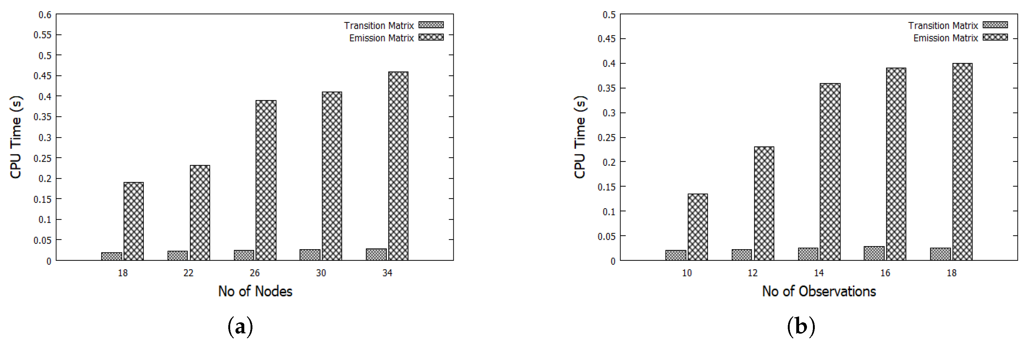
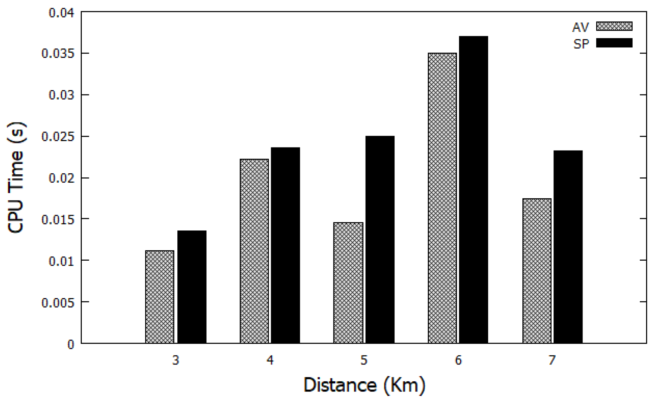
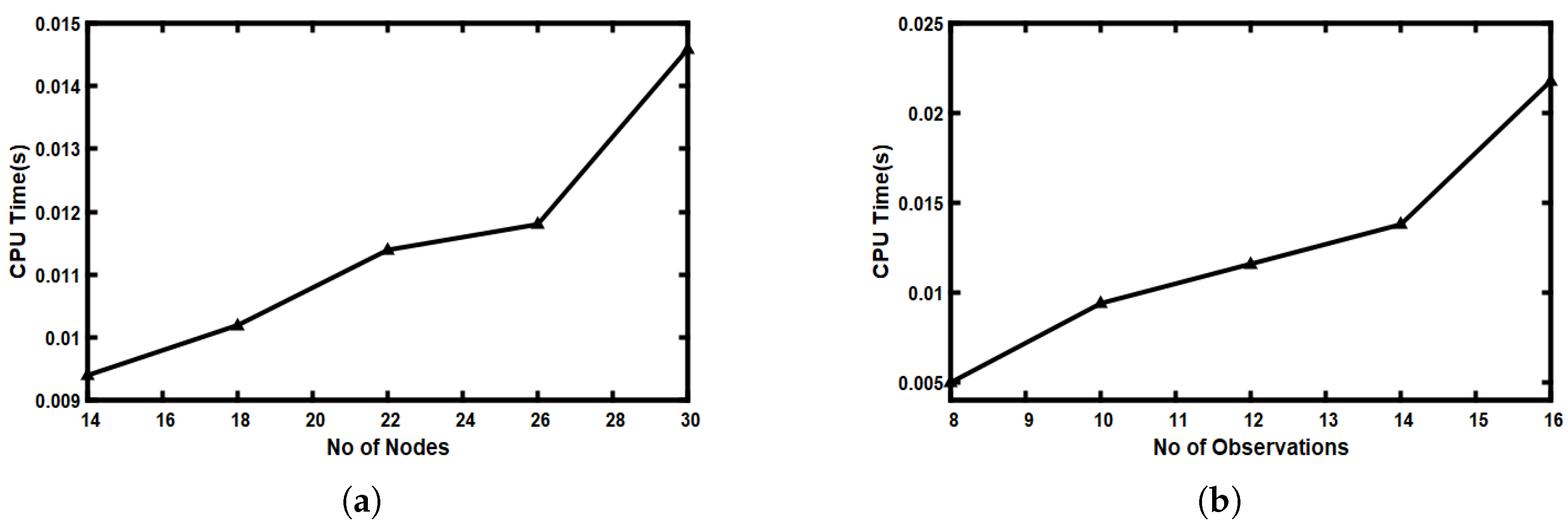
5.3. Adaptive Viterbi (AV) Evaluation

In this subsection, the performance of the proposed adaptive Viterbi (AV) algorithm is examined. Figure 4 compares, using different distances, the CPU time of the AV algorithm against the shortest path (SP) algorithm [32]. The distances range starts from around 2 km to 7 km. It is clear that the AV algorithm takes less CPU time compared to the SP algorithm. The AV algorithm can save about 38% time at most compared to SP algorithm. The AV algorithm calculations are depending on the transition matrix (A) and emission matrix (B), which are presented as inputs to the AV algorithm.

Figure 5 illustrates how changing the number of nodes and number of observations influences the CPU time of the AV algorithm, this is shown in Figure 5a,b, respectively. It is clear that by increasing both the number of nodes and the number of observations, the CPU time of the AV algorithm increases. This is expected as increasing both the number of nodes and the number of observations requires more computational time to compute the most likely path.

Figure 6 illustrates how varying the number of nodes and number of observations; Figure 6a,b respectively, affects the CPU time needed to construct both the transition matrix and emission matrix. The time of building the emission matrix is higher compared to the time of building the transition matrix. Furthermore, the CPU time of constructing both the emission matrix and transition matrix also increases by increasing the number of nodes. The CPU time of the emission matrix grows rapidly compared to the CPU time required by the transition matrix. This is due to the fact that increasing the number of nodes and the number of observations increases the size of both the transition matrix and the emission matrix and requires additional time to build them.

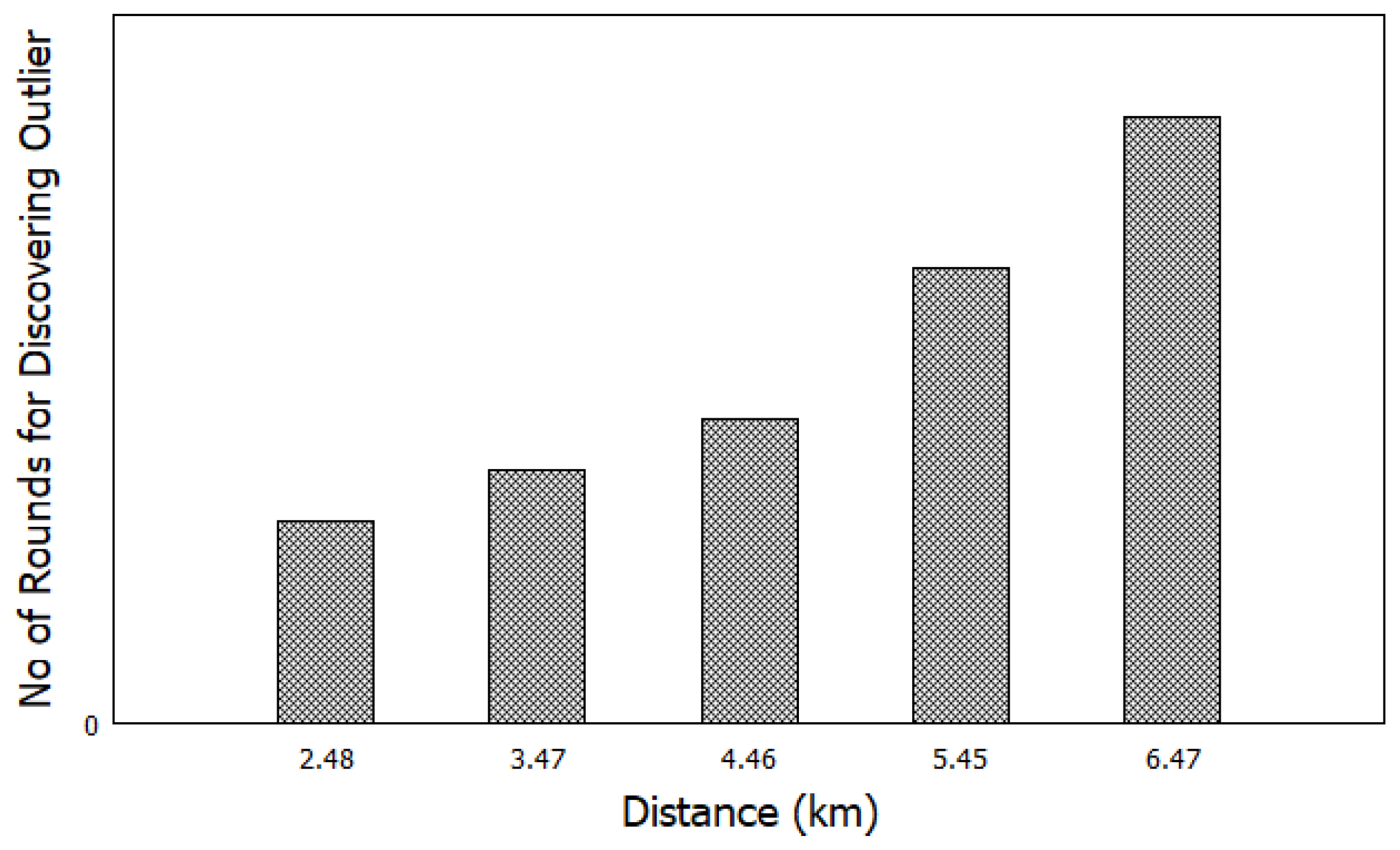
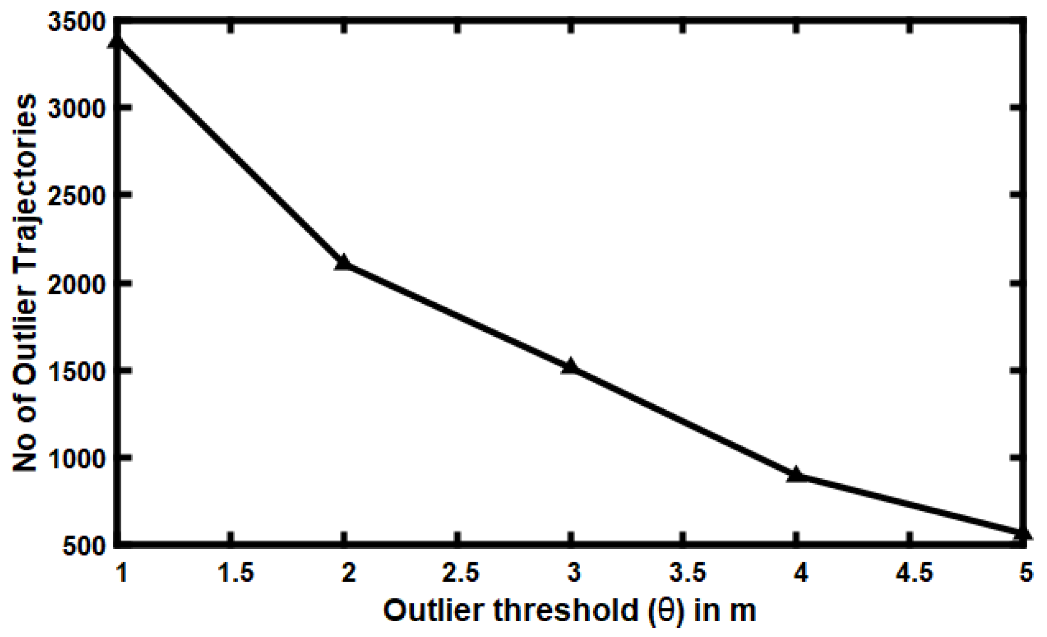
5.4. Impact of Varying Outlier Threshold ($\theta$)

In this experiment, the effect of using different values for the outlier threshold ($\theta$) parameter is measured against the number of discovered outlier trajectories. This experiment is conducted on trips with an average distance of approximately 6 km and 10 min as the average travel time of trips and set TW = 1 min. As shown in Figure 7, when the value of the outlier threshold increases the number of observed outlier trajectories is steadily decreased. Decreasing the outlier threshold placed more solid restrictions on the rideshare driver to complete the trip at the optimal time. The value of the outlier threshold changes depends on the required time for finishing the trip.

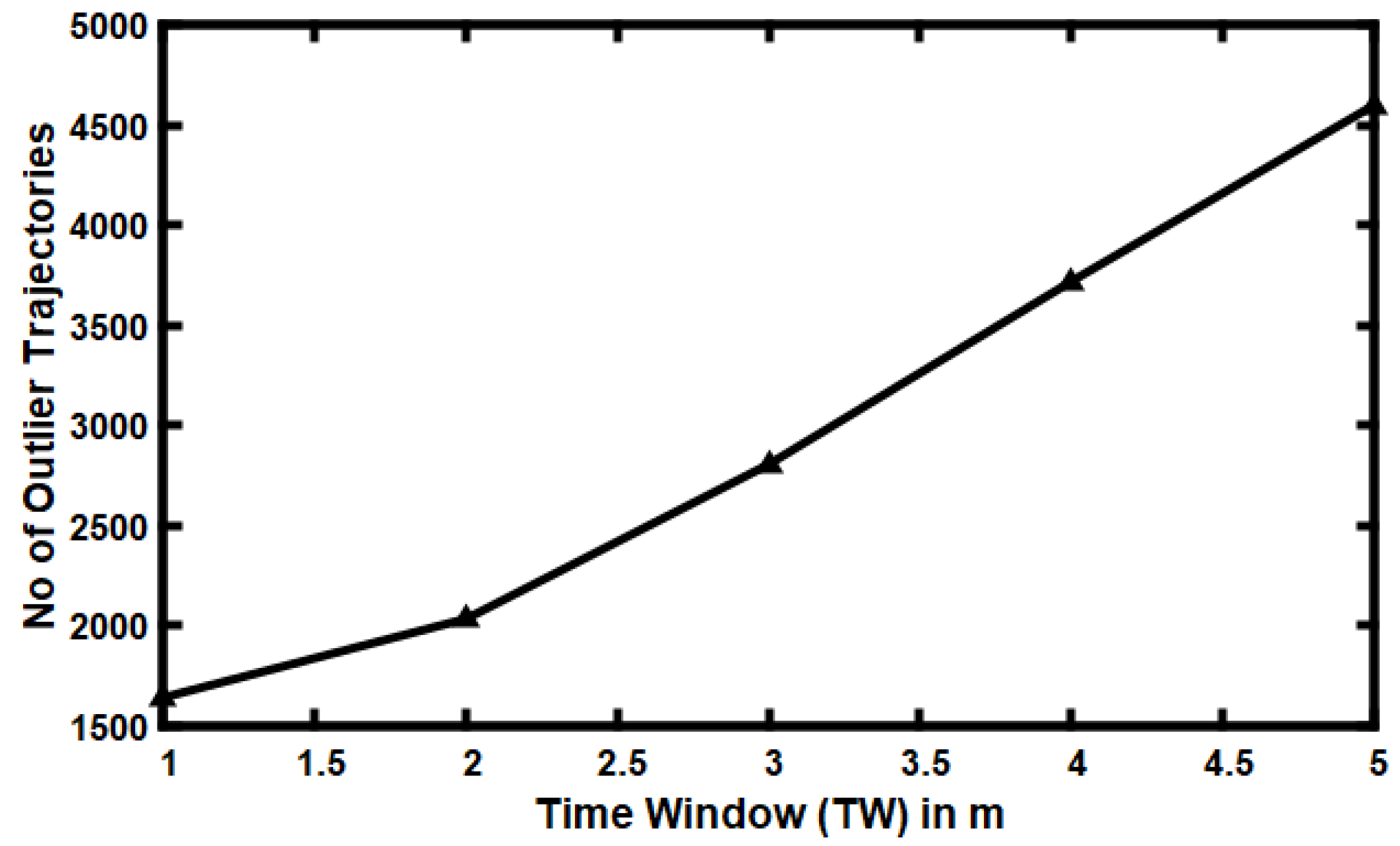
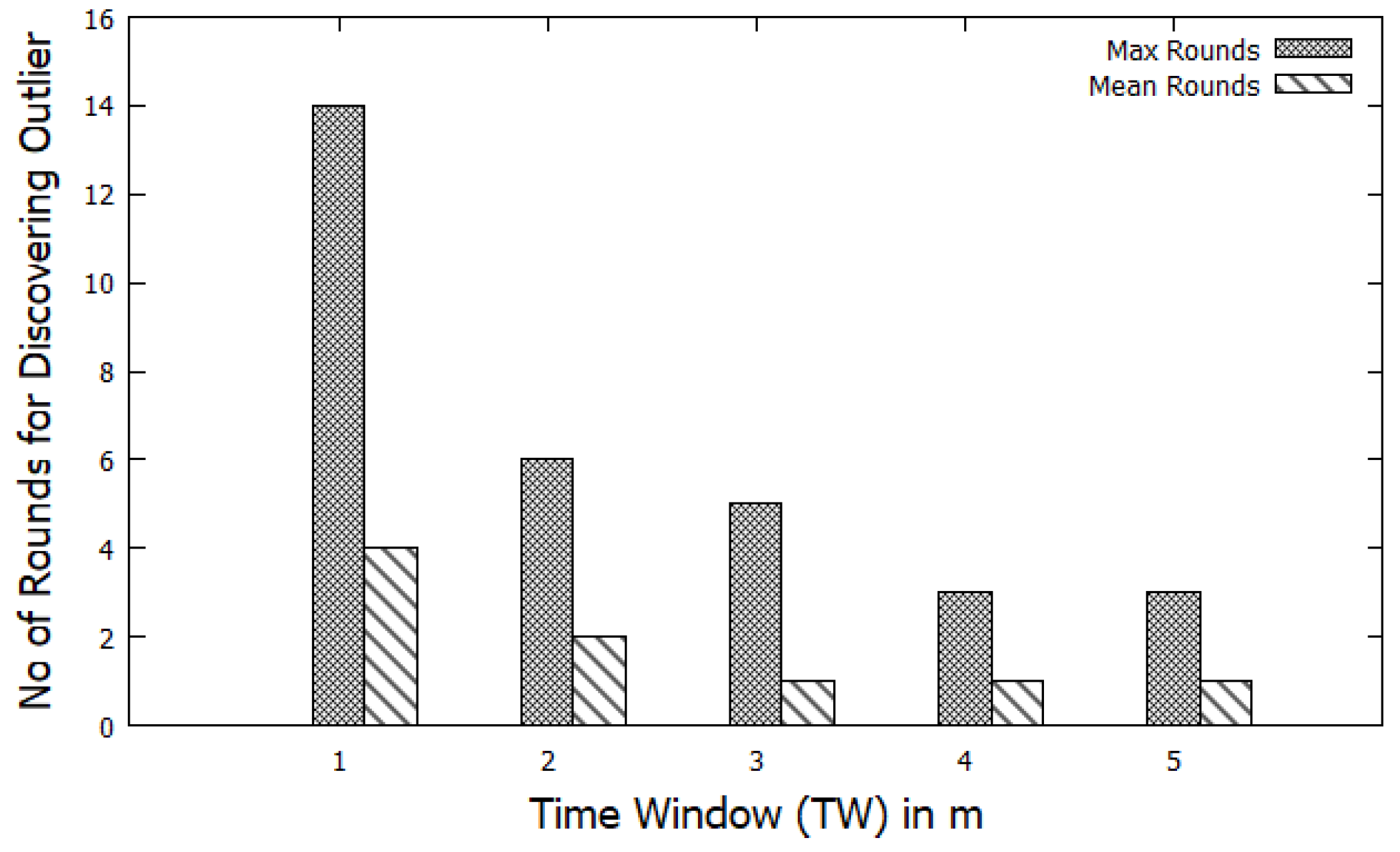
5.5. Impact of Varying Time Window (TW)

This experiment explores how the number of discovered outliers’ trajectories is affected by using various values for the time window parameter (TW). As illustrated in Figure 8, the X-axis represents the size of the time window in minutes, and Y-axis represents the number of discovered outliers’ trajectories. As shown in Figure 8, as the duration of the time window (TW) increases, the number of discovered outliers’ trajectories steadily increases; that is because raising the size of the time window increases the chance for a rideshare driver to move a longer distance of the total trip distance and increases the likelihood of spending more time than the ideal time.

The impacts of varying the time window (TW) scale is measured against the number of iterations required before finding outliers trajectories. As illustrated in Figure 9, the X-axis indicates the time window (TW) in minutes, and the Y-axis shows the number of checks needed to detect outlier trajectories. Both the maximum and the mean rounds required to discover outlier trajectories are measured. As seen in Figure 9, the number of rounds for discovering outliers’ trajectories decreases by increasing the duration of the time window (TW). Increasing the size of the time window requires a small number of re-examinations to discover outliers’ trajectories.

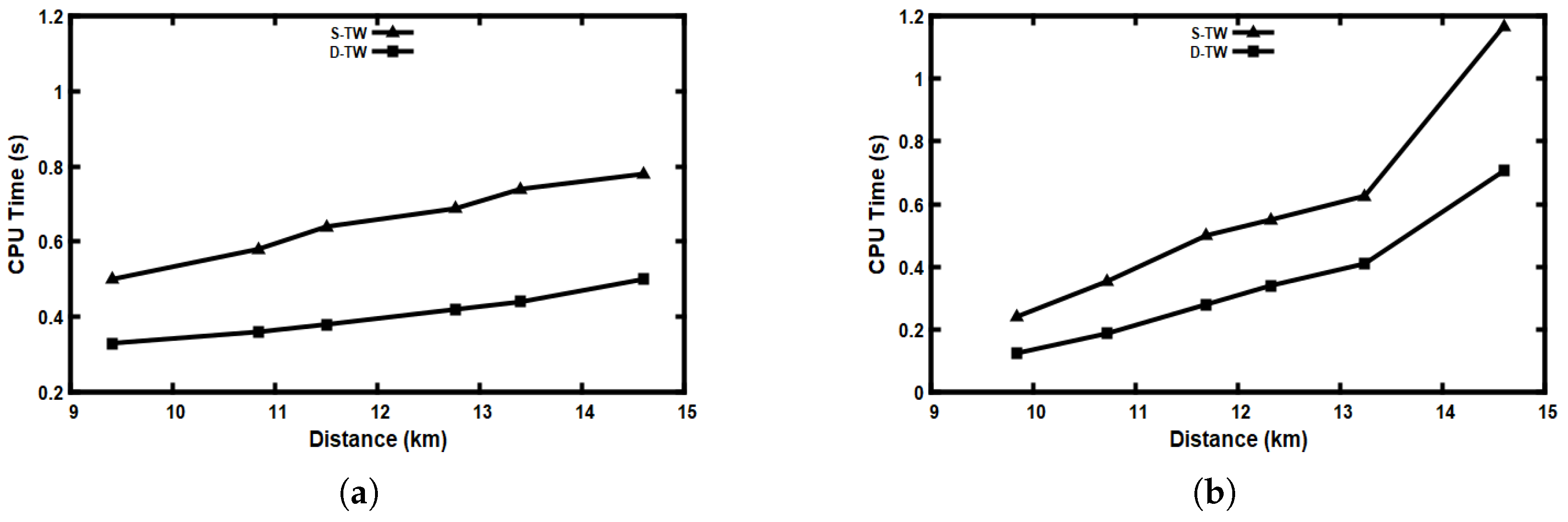
5.6. Performance Evaluation

In this part of the experiments, the CPU time of the proposed FraudMove algorithm was evaluated using different values for the time window (TW = 2 m, TW = 3 m, TW = 4 m, and outlier threshold $\theta$ = 2 m). The X-axis represents the distance between the source (S) and destination (D) of a trip in kilometers, and the Y-axis represents the CPU time in seconds elapsed until discovering outlier trajectories. Different distances were used from around 2 km to 8 km. As shown in Figure 10, increasing the distance also increases the computational time (CPU) for discovering outlier trajectories. Moreover, longer distances need more rounds to discover outlier trajectories. Furthermore, the CPU time decreases as the value of the time window (TW) increases, as this minimizes the number of attempts to discover outlier trajectories (as illustrated in Figure 10 when TW = 4 m).

Another experiment was conducted to measure the effect of varying the distance between the source (S) and destination (D) on the number of trials to discover outlier trajectories. The X-axis represents the distance between the source (S) and the destination (D) in kilometers. The Y-axis represents the number of rounds to discover outlier trajectories. As illustrated in Figure 11, the number of trials increases as the distance between the source (S) and the destination (D) increases—that is because increasing the distance requires further attempts to classify outlier trajectories.

In Figure 12, the CPU time for both static time window (S-TW) and dynamic time window (D-TW) using different distances is compared. Various distances were used starting from around 9 km to 15 km. A time window equal to 1 min was used for the static time window (S-TW). In Figure 12a, the outlier threshold ($\theta$) equals 1 m while in Figure 12b outlier threshold ($\theta$) equals 3 m. It is obvious that using a dynamic time window (D-TW) minimizes the CPU time of a FraudMove system, as seen in Figure 12a,b.

Figure 13 compares the CPU time of our proposed algorithm (FraudMove) and the OnATrade algorithm [15]. From Figure 13, we find that FraudMove is faster than the OnATrade algorithm. The explanation for that is that our algorithm saves time for checking every movement of a rideshare car and not check the outlier trajectory after each GPS point, similar to that in the OnATrade algorithm. Further, we find that the outlier path depends on time not similarity, similar to the OnATrade algorithm. Furthermore, FraudMove saves about 85% of the response time in a short distance. Moreover, it can reduce nearly 65% of response time in long distances.

5.7. Accuracy Evaluation

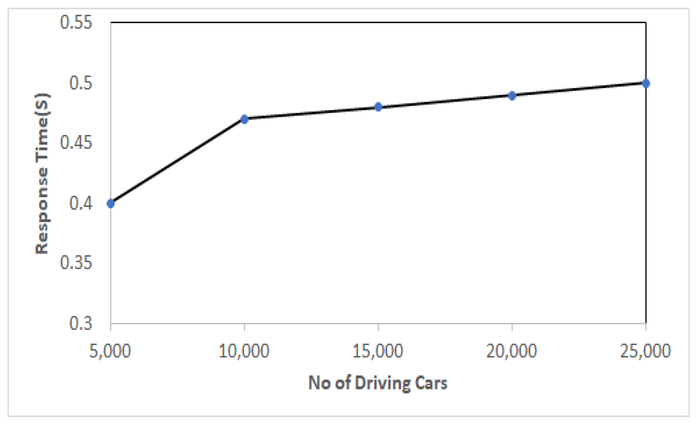
In this experiment, the accuracy of our proposed algorithm (FraudMove) and the OnATrade algorithm was compared. Figure 14 shows that compared to the OnATrade algorithm, the FraudMove algorithm observes a smaller number of outlier trajectories—that is because the OnATade algorithm generates a recommended paths for a given S and D on a rideshare trip. Once the readings of the GPS points deviate from the recommended routes, OnATade identifies this path as an outlier trajectory. On the other hand, the FraudMove algorithm evaluates a rideshare car path as an outlier once it takes more time than the time of the optimum route, which is more realistic.

Figure 15 describes an experiment that was introduced to clarify how varying the value of the outlier threshold ($\theta$) effects the determination of unexpected motions. The impact on performance was examined during the outlier threshold ($\theta$) increasing from 0.03 to 0.3 within the trip travel time. Overall, Figure 15 shows the receiver operating characteristic (ROC) curve of the FraudMove system. Indeed, this ROC curve is a continuous indicator that displays the continuous variables of a true positive rate (successfully identified outlier trajectories) and a false positive rate (normal trajectories identified as outliers). The result concludes that the FraudMove system achieves a high accuracy rate, which is approximately 95% in classifying outliers trips.

5.8. Scalability

This experiment examined the effect of increasing the number of rideshare cars on the response time of the algorithm. Figure 16 shows that there has been a slight increase in the response time for discovering outlier trajectories when the number of rideshare cars increases. The explanation for this is that raising the number of requests from a larger number of rideshare vehicles often expanded the queue to answer such queries. This experiment consisted of 25,000 similar rideshare cars. Starting from 5000 rideshare cars, we grew the size of a rideshare car four times by joining 5000 trips each time and closing up with rideshare cars with a size of 25,000. When the number of rideshare cars is 5000, the response time = 0.4 s, while on rideshare cars with a size of 25,000, the response time = 0.5 s; this shows that the average response time was raised by approximately 2.5% for each rise in the size of rideshare cars. That means a FraudMove algorithm is scalable enough for handling a larger number of rideshare car queries simultaneously.

6. Discussion

In summary, the results show that the FraudMove system achieves a higher accuracy rate with less processing time. As a result, the FraudMove system is an effective system for helping the real-time detection of fraud drivers. Additionally, FraudMove motivates researchers who are excited about discovering transportation problems [34] and in the different causes for trip delays.

• Urban traffic detection: discovering outlier trajectories from GPS traces is an attractive topic for finding congested roads. A traffic flow can be recognized by examining moving objects trajectories in urban cities. Traffic flow detection is an essential task in planning smart cities and transportation management.
• Discovering road problems: identifying route problems such as closed roads for emergency conditions (e.g., events, accidents, bad weather, and potholes) is required for finding alternative routes for drivers. Generally, poor driving surfaces are caused by a combination of seasonal and traffic conditions.

7. Conclusions

In this paper, FraudMove system is proposed for the real-time discovery of fraud drivers by detecting the outlier trajectories of these drivers based on the time factor. Mainly, FraudMove depends on travel time to identify the outlier trajectory. Furthermore, FraudMove employed an adaptive Viterbi (AV) algorithm to compute the most probable path of a trip. Moreover, FraudMove used a tunable time window parameter to minimize the computation cost of the outlier detection process. The power of FraudMove lies in identifying fraud drivers and anomalous traffic conditions with high accuracy and achieving a fast query response time. In the end, our experimental results, based on real trajectory data, prove that FraudMove achieved high classification accuracy results with a minimal response time.

References

1. Business of Apps. Uber Revenue and Usage Statistics; Business of Apps. 2020. Available online: https://www.businessofapps.com/data/uber-statistics/ (accessed on 1 September 2021).
2. Yuan, J.; Zheng, Y.; Zhang, C.; Xie, W.; Xie, X.; Sun, G.; Huang, Y. T-drive: Driving directions based on taxi trajectories. In Proceedings of the 18th ACM SIGSPATIAL International Symposium on Advances in Geographic Information Systems, San Jose, CA, USA, 2–5 November 2010. [Google Scholar]
3. Zheng, Y.; Zhang, L.; Xie, X.; Ma, W.Y. Mining interesting locations and travel sequences from GPS trajectories. In Proceedings of the 18th International Conference on World Wide Web, Madrid, Spain, 20–24 April 2009; pp. 791–800. [Google Scholar]
4. Liu, L.; Andris, C.; Ratti, C. Uncovering cabdrivers’ behavior patterns from their digital traces. Comput. Environ. Urban Syst. 2010, 34, 541–548. [Google Scholar] [CrossRef]
5. Calabrese, F.; Colonna, M.; Lovisolo, P.; Parata, D.; Ratti, C. Real-time urban monitoring using cell phones: A case study in Rome. IEEE Trans. Intell. Transp. Syst. 2010, 12, 141–151. [Google Scholar] [CrossRef]
6. Zhu, J.; Jiang, W.; Liu, A.; Liu, G.; Zhao, L. Effective and efficient trajectory outlier detection based on time-dependent popular route. World Wide Web 2017, 20, 111–134. [Google Scholar] [CrossRef]
7. Chen, C.; Zhang, D.; Castro, P.S.; Li, N.; Sun, L.; Li, S.; Wang, Z. iBOAT: Isolation-Based Online Anomalous Trajectory Detection. IEEE Trans. Intell. Transp. Syst. 2013, 14, 806–818. [Google Scholar] [CrossRef]
8. Zheng, Y.; Liu, Y.; Yuan, J.; Xie, X. Urban computing with taxicabs. In Proceedings of the 13th International Conference on Ubiquitous Computing, Beijing, China, 17–21 September 2011; pp. 89–98. [Google Scholar]
9. Zheng, Y.; Liu, L.; Wang, L.; Xie, X. Learning transportation mode from raw gps data for geographic applications on the web. In Proceedings of the 17th International Conference on World Wide Web, Beijing, China, 21–25 April 2008; pp. 247–256. [Google Scholar]
10. Zheng, Y. Trajectory Data Mining: An Overview. ACM Trans. Intell. Syst. Technol. 2015, 6, 1–41. [Google Scholar] [CrossRef]
11. Sun, L.; Zhang, D.; Chen, C.; Castro, P.S.; Li, S.; Wang, Z. Real time anomalous trajectory detection and analysis. Mob. Netw. Appl. 2013, 18, 341–356. [Google Scholar] [CrossRef]
12. Zhang, D.; Li, N.; Zhou, Z.H.; Chen, C.; Sun, L.; Li, S. iBAT: Detecting anomalous taxi trajectories from GPS traces. In Proceedings of the 13th International Conference on Ubiquitous Computing, Beijing, China, 17–21 September 2011. [Google Scholar]
13. Zhu, J.; Jiang, W.; Liu, A.; Liu, G.; Zhao, L. Time-Dependent Popular Routes Based Trajectory Outlier Detection. In International Conference on Web Information Systems Engineering; Springer: Cham, Switzerland, 2015. [Google Scholar]
14. Lee, J.G.; Han, J.; Li, X. Trajectory Outlier Detection: A Partition-and-Detect Framework. In Proceedings of the IEEE 24th International Conference on Data Engineering, Cancun, Mexico, 7–12 April 2008. [Google Scholar]
15. Zhou, Z.; Dou, W.; Jia, G.; Hu, C.; Xu, X.; Wu, X.; Pan, J. A method for real-time trajectory monitoring to improve taxi service using GPS big data. Inf. Manag. 2016, 53, 964–977. [Google Scholar] [CrossRef] [Green Version]
16. Chen, Z.; Shen, H.T.; Zhou, X. Discovering popular routes from trajectories. In Proceedings of the 2011 IEEE 27th International Conference on Data Engineering, Hannover, Germany, 11–16 April 2011; pp. 900–911. [Google Scholar]
17. Li, S.Z.; Jain, A. (Eds.) Viterbi Algorithm. In Encyclopedia of Biometrics; Springer: Boston, MA, USA, 2009; p. 1376. [Google Scholar] [CrossRef]
18. Liu, Z.; Pi, D.; Jiang, J. Density-based trajectory outlier detection algorithm. J. Syst. Eng. Electron. 2013, 24, 335–340. [Google Scholar] [CrossRef]
19. Ge, Y.; Xiong, H.; Zhou, Z.H.; Ozdemir, H.; Yu, J.; Lee, K.C. Top-Eye: Top-k evolving trajectory outlier detection. In Proceedings of the 19th ACM International Conference on Information and Knowledge Management, Toronto, ON, Canada, 26–30 October 2010. [Google Scholar]
20. Ge, Y.; Xiong, H.; Liu, C.; Zhou, Z.H. A Taxi Driving Fraud Detection System. In Proceedings of the IEEE 11th International Conference on Data Mining, Vancouver, BC, Canada, 11–14 December 2011. [Google Scholar]
21. Kong, X.; Song, X.; Xia, F.; Guo, H.; Wang, J.; Tolba, A. LoTAD: Long-term traffic anomaly detection based on crowdsourced bus trajectory data. World Wide Web 2018, 21, 825–847. [Google Scholar] [CrossRef]
22. Breunig, M.M.; Kriegel, H.P.; Ng, R.T.; Sander, J. LOF: Identifying Density-Based Local Outliers. In Proceedings of the 2000 ACM SIGMOD International Conference on Management of Data, Dallas, TX, USA, 15–18 May 2000. [Google Scholar]
23. Eldawy, E.O.; Mokhtar, H.M. Clustering-Based Trajectory Outlier Detection. Int. J. Adv. Comput. Sci. Appl. 2020, 11, 133–139. [Google Scholar] [CrossRef]
24. Liu, F.T.; Ting, K.M.; Zhou, Z.H. Isolation-based anomaly detection. ACM Trans. Knowl. Discov. Data (TKDD) 2012, 6, 1–39. [Google Scholar] [CrossRef]
25. Kanoulas, E.; Du, Y.; Xia, T.; Zhang, D. Finding fastest paths on a road network with speed patterns. In Proceedings of the IEEE 22nd International Conference on Data Engineering (ICDE’06), Atlanta, GA, USA, 3–7 April 2006; p. 10. [Google Scholar]
26. Gonzalez, H.; Han, J.; Li, X.; Myslinska, M.; Sondag, J.P. Adaptive fastest path computation on a road network: A traffic mining approach. In Proceedings of the 33rd International Conference on Very Large Data Bases, VLDB 2007, Vienna, Austria, 23–27 September 2007; Association for Computing Machinery, Inc.: New York, NY, USA, 2007; pp. 794–805. [Google Scholar]
27. Sacharidis, D.; Patroumpas, K.; Terrovitis, M.; Kantere, V.; Potamias, M.; Mouratidis, K.; Sellis, T. On-line discovery of hot motion paths. In Proceedings of the 11th International Conference on Extending Database Technology: Advances in Database Technology, Nantes, France, 25–29 March 2008; pp. 392–403. [Google Scholar]
28. Luo, W.; Tan, H.; Chen, L.; Ni, L.M. Finding time period-based most frequent path in big trajectory data. In Proceedings of the 2013 ACM SIGMOD International Conference on Management of Data, New York, NY, USA, 22–27 June 2013; pp. 713–724. [Google Scholar]
29. Rabiner, L.; Juang, B. An introduction to hidden Markov models. IEEE Assp Mag. 1986, 3, 4–16. [Google Scholar] [CrossRef]
30. Castro, P.S.; Zhang, D.; Chen, C.; Li, S.; Pan, G. From taxi GPS traces to social and community dynamics: A survey. ACM Comput. Surv. (CSUR) 2013, 46, 1–34. [Google Scholar] [CrossRef]
31. Haklay, M.; Weber, P. Openstreetmap: User-generated street maps. IEEE Pervasive Comput. 2008, 7, 12–18. [Google Scholar] [CrossRef] [Green Version]
32. Johnson, D.B. A note on Dijkstra’s shortest path algorithm. J. ACM (JACM) 1973, 20, 385–388. [Google Scholar] [CrossRef]
33. Piorkowski, M.; Sarafijanovic-Djukic, N.; Grossglauser, M. CRAWDAD Data Set Epfl/Mobility (v. 2009-02-24). 2009. [Google Scholar]
34. Meng, F.; Yuan, G.; Lv, S.; Wang, Z.; Xia, S. An overview on trajectory outlier detection. Artif. Intell. Rev. 2018, 52, 2437–2456. [Google Scholar] [CrossRef]
Figure 1. Example on shortest path in road network graph.
Ijgi 10 00767 g001
Figure 2. FraudMove architecture.
Ijgi 10 00767 g002
Figure 3. Steps in transition graph of AV example: (a) transition graph; (b) transition graph with probabilities; (c) transition graph with probabilities and best path in red line.
Ijgi 10 00767 g003
Figure 4. Comparison of CPU time between AV and SP using different distances.
Ijgi 10 00767 g004
Figure 5. Effects of varying number of nodes and number of observations on CPU time of AV algorithm: (a) varying number of nodes; (b) varying number of observations.
Ijgi 10 00767 g005
Figure 6. Effects of varying number of nodes and number of observations on CPU time of constructing the Transition matrix and Emission matrix: (a) varying number of nodes; (b) varying number of observations.
Ijgi 10 00767 g006
Figure 7. Effects of varying the outlier threshold ( θ ) on the number of discovered outliers’ trajectories.
Ijgi 10 00767 g007
Figure 8. Effects of varying the time window (TW) on the number of discovered outliers’ trajectories.
Ijgi 10 00767 g008
Figure 9. Effects of varying the time window (TW) on the number of rounds to discovered outliers’ trajectories.
Ijgi 10 00767 g009
Figure 10. CPU time for different distances.
Ijgi 10 00767 g010
Figure 11. Effects of varying distances between S-D on the number of rounds to discovered outliers’ trajectories.
Ijgi 10 00767 g011
Figure 12. Comparison between CPU time of S-TW and D-TW using different distances: (a) outlier threshold ( θ ) = 1 m; (b) outlier threshold ( θ ) = 3 m.
Ijgi 10 00767 g012
Figure 13. Comparing FraudMove to OnATrade (performance).
Ijgi 10 00767 g013
Figure 14. Comparing FraudMove to OnATrade (accuracy).
Ijgi 10 00767 g014
Figure 15. The ROC curve of FraudMove.
Ijgi 10 00767 g015
Figure 16. Effects of varying the number of driving cars on response time.
Ijgi 10 00767 g016