Mapping Seasonal High-Resolution PM_2.5 Concentrations with Spatiotemporal Bagged-Tree Model across China

Abstract

High concentrations of fine particulate matter (PM_2.5) are well known to reduce environmental quality, visibility, atmospheric radiation, and damage the human respiratory system. Satellite-based aerosol retrievals are widely used to estimate surface PM_2.5 levels because satellite remote sensing can break through the spatial limitations caused by sparse observation stations. In this work, a spatiotemporal weighted bagged-tree remote sensing (STBT) model that simultaneously considers the effects of aerosol optical depth, meteorological parameters, and topographic factors was proposed to map PM_2.5 concentrations across China that occurred in 2018. The proposed model shows superior performance with the determination coefficient (R²) of 0.84, mean-absolute error (MAE) of 8.77 μg/m³ and root-mean-squared error (RMSE) of 15.14 μg/m³ when compared with the traditional multiple linear regression (R² = 0.38, MAE = 18.15 μg/m³, RMSE = 29.06 μg/m³) and linear mixed-effect (R² = 0.52, MAE = 15.43 μg/m³, RMSE = 25.41 μg/m³) models by the 10-fold cross-validation method. The results collectively demonstrate the superiority of the STBT model to other models for PM_2.5 concentration monitoring. Thus, this method may provide important data support for atmospheric environmental monitoring and epidemiological research.

1. Introduction

Particulate matter with ≤2.5 μm diameter is called fine particulate matter (PM_2.5) [1]. Numerous epidemiological studies have found that cardiovascular and respiratory diseases are closely related to long-term exposure to PM_2.5 [2]. Emerging evidence has also shown that PM_2.5 is associated with impaired cognitive function [3], Alzheimer’s disease, Parkinson’s disease, cognitive decline, and dementia [4,5]. High resolution and high coverage PM_2.5 levels promote epidemiologists to analysis the effects of PM_2.5 in human health with more efficient [6]. Unfortunately, the lack of accurate monitoring data on long-term PM_2.5 levels results in scarcity of epidemiological studies concerning the impact of particulate matter on human health [7]. The uneven atmospheric monitoring network of the China Meteorological Administration, established in 2013, cannot capture the regional PM_2.5 concentration. Thus, establishing a suitable PM_2.5 model with wide-area coverage is necessary.

Aerosol optical depth (AOD) is an important parameter in atmospheric research [8]. AOD can be calculated by integrating aerosol extinction coefficient in a vertical column of atmosphere. In recent years, an aerosol robot network (AERONET) has been established in China, which can monitor AOD values relatively accurately and support regionally environmental analysis. However, the sparse distribution of monitoring stations makes it difficult to characterize the actual spatial change of AOD [9]. Satellite remote sensing can realize wide-area aerosol retrieval, thereby providing chances for large-scale regional air quality assessments [10]. Numerous studies have demonstrated a complex correlation between AOD and surface PM_2.5 levels. Surface PM_2.5 concentrations estimated by satellite-based AOD have been widely applied in recent years to monitor air quality [10,11]. The AOD products commonly used to estimate PM_2.5 concentrations include MODIS AOD [12,13], MERRA-2 AOD, and Himawari-8 AOD [14,15]. A new high-resolution (1 km) daily MCD19A2 AOD retrieved by a multiangle implementation of atmospheric correction (MAIAC) algorithm was released on 30 May 2018 [16]. In the MAIAC AOD product development process, researchers improved many key operations, such as snow and cloud screening and selecting aerosol types after analysis based on time series images. At present, MAIAC AOD data have been widely used to reveal the changes of AOD in various regions of the world [17]. However, for estimating fine particle concentrations on fine scale, higher resolution AOD products are indispensable, and the resolution of AOD data often used in previous studies cannot meet the requirements. Based on this situation, the VIIRS sensor was initiated with the launch of the S-NPP satellite in 2011. It is a new generation of satellite sensor used to describe aerosol characteristics [18]. As a scanning radiometer, it has expanded and improved capabilities when compared with the traditional AVHRR and MODIS sensors [18], and can generate aerosol products with a spatial resolution of 750 m [19].

The methods for estimating PM_2.5 concentrations based on satellite remote sensing mainly include the empirical formula [20], chemical transport model [12], and statistical model. The classical statistical models include the linear mixed-effect (LME) model, the generalized additive model, and the geographical-weighted regression model [12,21,22,23]. A large number of PM_2.5 concentration data from ground monitoring stations are required to develop and verify these models [7]. However, these models are unable to completely capture the complex relations of PM_2.5 with various influencing factors [24] and cannot fully reflect temporal and spatial differences in PM_2.5 distributions. Thus, developing superior model to map PM_2.5 concentrations is still an important task by respectively considering the spatio-temporal heterogeneity of different variables.

In this study, the AOD products with high coverage ratio are generated by integrating MODIS MAIAC AOD [13] and VIIRS IP AOD [25]. Integrating the advantages of the two AOD products by considering similar pixels between the two products can improve the coverage of MAIAC AOD products. Moreover, a spatiotemporal bagged-tree (STBT) model that considers the spatiotemporal heterogeneity between different influencing factors was applied to map PM_2.5 concentrations across China that occurred in 2018. Sample-based and station-based cross-validation (CV) methods are used to evaluate the performance of the STBT model.

2. Study Area and Datasets

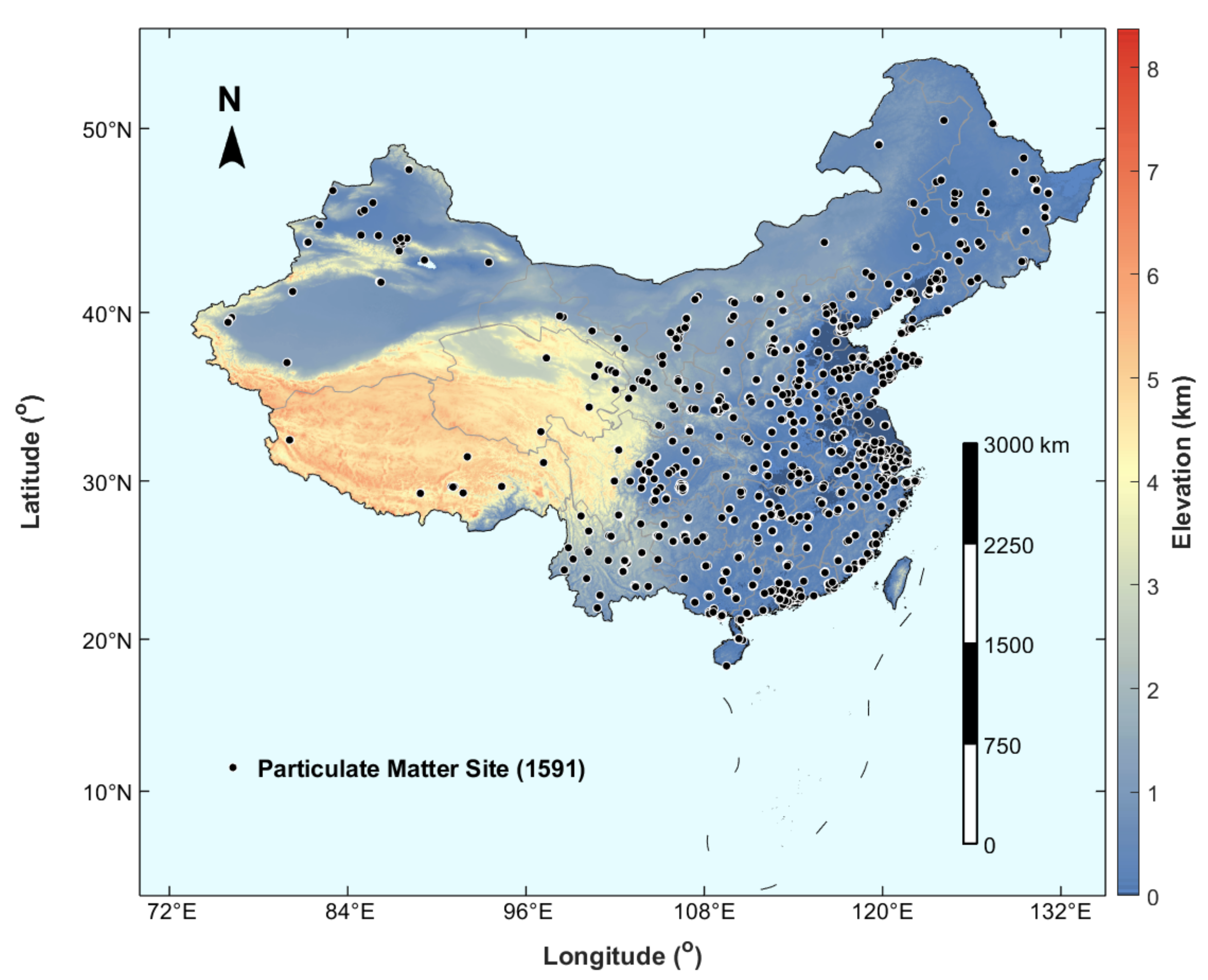
Ground PM_2.5 observation, MAIAC AOD, VIIRS IP AOD, meteorological parameters, topographic factors, and other auxiliary data related to site-measured PM_2.5 levels were applied in this study, as shown in

Table 1. Datasets used in this study. AOD: aerosol optical depth; RH: relative humidity; TEMP: temperature; WS: wind speeds; BLH: boundary layer height; NDVI: normalized difference vegetation; DEM: digital elevation model.

Data	Variables	Unit	Temporal Resolution	Spatial Resolution	Sources
PM2.5	PM2.5	µg/m3	1 h	site	CNEMC
MAIAC AOD	AOD	Unitless	1 day	1 km	MODIS
VIIRS IP AOD	AOD	Unitless	1 day	750 m	S-NPP
Meteorological parameters	RH	%	1 h	0.25°	ERA5
	TEMP	K	1 h	0.25°
	WS	m/s	1 h	0.25°
	BLH	m	1 h	0.25°
Topographic factors	DEM	m	--	90 m	USGS
Vegetation factors	NDVI	Unitless	16 days	0.05°	MODIS

. The datasets cover the period from 1 January to 31 December 2018.

2.1. Study Area

In this study, the nationwide PM_2.5 observation data at 1591 sites were downloaded from the database of the China National Environmental Monitoring Center. As shown in Figure 1, the monitoring sites are distributed unevenly in the study area; specifically, the stations are densely distributed in the east and sparsely distributed in the west. East China is adjacent to the Pacific Ocean, which spans many temperature zones, such as tropical, subtropical, and temperate monsoon. In contrast, the northwest belongs to a non-monsoon region with a temperate continental climate.

2.2. MODIS AOD

The MODIS AOD product has high retrieval accuracy and is widely applied for PM_2.5 level monitoring over large areas [26]. The MAIAC AOD product developed by the MAIAC algorithm has a high spatial resolution of 1 km. The confidence level of the MAIAC AOD product used in this study is high. MAIAC AOD from 1 January 2018 to 31 December 2018 were downloaded from NASA (http://ladsweb.modaps.eosdis.nasa.gov/, accessed on 2 February 2019).

2.3. VIIRS IP AOD

The visible infrared imaging radiometer (VIIRS), which is extended from the MODIS series, was carried on the S-NPP satellite [27] and used to obtain the AOD product with 750 m resolution. The VIIRS IP AOD has been used in domestic and international studies to retrieve PM_2.5 concentrations over large areas [28]. VIIRS IP AOD from 1 January 2018 to 31 December 2018 were downloaded from NOAA (https://ncc.nesdis.noaa.gov/VIIRS/, accessed on 11 April 2019).

2.4. Meteorological Data

The surface PM_2.5 concentrations were closely related to meteorological parameters, especially the boundary layer height and the wind [29]. In this study, the meteorological data from the reanalysis dataset of the European Meteorological Centre are used in this study. These data were downloaded from ERA5 (https://cds.climate.copernicus.eu/cdsapp#!/home, accessed on 22 June 2019). The meteorological parameters used in this study, including relative humidity (RH), temperature (TEMP), boundary layer height (BLH), and wind speed (WS), as shown in Table 1.

2.5. Geographic and Topographic Data

MODIS retrieved Normalized difference vegetation index (NDVI) with a time resolution of 16 days was used in this study, which can represent different land cover types. NDVI data at a spatial resolution of 0.05° were downloaded from the NASA Earth Observatory (http://neo.sci.gsfc.nasa.gov/, accessed on 17 June 2019). In addition, digital elevation model (DEM) data from the U.S. Geological Survey (https://www.usgs.gov/, accessed on 18 April 2018) with a spatial resolution 30 m was used in this study to characterize the topographic features of the study area.

3. Methodology

3.1. Multi-Source AOD Data Fusion

Given cloud effect and MODIS aerosol retrieval method, a large number of AOD data are missing in the study area. According to the mechanism of retrieving aerosol loadings from satellite-based sensors, some researchers considered the relationship between AOD loadings and NDVI, comprehensively weighing the spatial proximity, AOD and NDVI similarity, to recover AOD [30,31]. The VIIRS IP AOD at 550 nm can provide a reliable dataset with a high resolution (750 m) [32]. In this study, filling AOD vacancy based on the adaptive threshold method was adopted to enhance the spatiotemporal continuity of the data. The similar pixels from VIIRS IP AOD found by local range were used to recover missing pixels in the MAIAC AOD product. Here, adaptive determination was used to search for similar pixels by considering local differences between MAIAC AOD and VIIRS IP AOD values and spatial distance. Similar pixels should satisfy the following inequality,

$$|A_j-A_i|\le A\_thi,$$

(1)

where $A_j$ and $A_i$ refer to a similar AOD pixel and target AOD pixel in the VIIRS IP AOD dataset, respectively, and $A\_thi$ is the adaptive threshold calculated by the AOD local standard deviation formula:

$$A\_thi=std(MAIACdiv-VIIRSdiv)*length*width,$$

(2)

where $MAIACdiv$ and $VIIRSdiv$ refer to two AOD datasets from MAIAC and VIIRS in a given window respectively, $std$ represents the calculated standard deviation, and $length$ and $width$ represent the local window size. Similar pixels are endowed with weights based on AOD differences and spatial relations:

$$D_{ij}=|A_j-A_i+\beta |*\left({\left(x_j-x_i\right)}^2+{\left(y_j-y_i\right)}^2\right),$$

(3)

where $x \mathrm{and} y$ refer to longitude and latitude, respectively, and $\beta$ is a small value that prevents $Dij$ from equaling zero, which is empirically determined. Normalized processing is then carried out:

$$W_{ij}=\frac{1/D_{ij}}{{\displaystyle {\sum }_{i=1}^N\left(1/D_{ij}\right)}},$$

(4)

Finally, the missing value in MAIAC AOD is filled based on the weighting sum of these similar pixels in MAIAC AOD that are determined by the similarity relation between MAIAC and VIIRS AOD:

$$AO{D}_{tg}={\displaystyle {\sum }_{i=1}^N{W}_{ij}*AO{D}_i},$$

(5)

3.2. Spatiotemporal Bagged-Tree Model

3.2.1. Bagged-Tree Model

Decision tree models typically give good classification decisions [33]. The model is built in the light of the bagged-tree combination classification method [34]. The combined classifier used in this work is composed of multiple individual classifiers consisting of decision trees. The training data of each tree are extracted by using bootstrap. Each individual classifier has its own classification results. The classified result from the combined classifier is determined by the combination of the results of individual classifiers to avoid overfitting.

3.2.2. Spatiotemporal Weighted Function

The spatial cross-correlation and temporal autocorrelation of the data were explored by considering the spatio-temporal heterogeneity of PM_2.5 concentrations in this study. The spatial cross-correlation can be expressed by the spatial weight function:

$$P_s=\frac{{\displaystyle {\sum }_{w=1}^W\frac{1}{d_{s_w}{}^2}P{M}_w}}{{\displaystyle {\sum }_{w=1}^W\frac{1}{d_{s_w}{}^2}}},$$

(6)

where $d_s$ refers to the space distance, $P{M}_w$ refers to the PM_2.5 of station w adjacent to the target station, and W refers to the number of stations within the selected scope. The temporal autocorrelation is expressed by the temporal weight function:

$$P_t=\alpha {\displaystyle {\sum }_{t-1}^{\mathrm{t}+1}P{M}_{\mathrm{t}}}+\beta \frac{1}{n}{\displaystyle {\sum }_1^{n}P{M}_n}+\gamma \frac{1}{m}{\displaystyle {\sum }_1^{m}P{M}_M}+\theta ,$$

(7)

where $P{M}_t$ refers to the PM_2.5 measured in the day before and after the current day, $\frac{1}{n}{\displaystyle {\sum }_1^{n}P{M}_n}$ is the averaged PM_2.5 value within a week, n is the number of valid days of the week, $\frac{1}{m}{\displaystyle {\sum }_1^{m}P{M}_M}$ represents the averaged PM_2.5 level within a month, and m is the number of valid days of the month. The coefficient is obtained by linear analysis, and $\theta$ refers to the linear analysis residual.

3.3. Other Models

3.3.1. MLR Model

The simple multiple linear regression (MLR) model can be expressed as:

$$\begin{array}{c}P{M}_{2.5}=b+a_1\times AOD+a_2\times TEMP+a_3\times RH+a_4\times WS\\ +a_5\times BLH+a_6\times NDVI+a_7\times DEM+\epsilon \end{array}$$

(8)

where b indicates the intercept, ${\alpha }_1-{\alpha }_7$ refer to regression coefficients, and ε represents the error term.

3.3.2. LME Model

The ordinary MLR model can be extended as LME model by considering random effect in a specific time. LME model can explain the time-related relationship between surface PM_2.5 levels and multiple predictors in a specific region, and can be expressed as:

$$\begin{array}{r}P{M}_{2.5}{}_{n,m}=[{\beta }_0+b_{0,n,m}^{day}]+[{\beta }_1+b_{1,n,m}^{day}]\times AO{D}_{n,m}+{\beta }_2\times TEM{P}_{n,m}+{\beta }_3\times R{H}_{n,m}\\ +{\beta }_4\times W{S}_{n,m}+{\beta }_5\times BL{H}_{n,m}+{\beta }_6\times NDV{I}_{n,m}+{\beta }_7\times DE{M}_{n,m}+{\epsilon }_{n,m};\\ (b_{0,n,m}^{day},b_{1,n,m}^{day})~N[(0,0,\sum )],{\epsilon }_{n,m}~N(0,{\sigma }^2);\end{array}$$

(9)

where n and m refers to the grid and time index, respectively; β₀ represent the fixed intercept; ${\beta }_1-{\beta }_7$ are the fixed slopes for these corresponding predictors; $b_{1,n,m}^{day}$ and $b_{0,n,m}^{day}$ represent the time-specific random slope and intercept for intercept and AOD, respectively; $\sum$ indicates the variance–covariance matrix of the random effects; ${\epsilon }_{n,m}$ represent the error term.

3.4. Model Evaluation

The performance of the proposed STBT model was validated via sample-based and station-based 10-fold cross-validation (CV) methods to calculate the determination coefficient (R²), MAE, and RMSE. CV has an ability to reveal whether or not a model is overfit. Finally, the results of the proposed model were compared with those of traditional estimation models, such as the MLR and LME models, to determine its accuracy and generalizability.

4. Results and Discussion

4.1. Assessment of Fused AOD and Statistical Analysis of the Datasets

4.1.1. Assessment of Fused AOD

The AERONET measurements are used to evaluate the fused AOD data. However, AERONET network observes AOD value in multiple wavelengths, almost of which are different from MAIAC AOD at 550 nm. Therefore, AERONET aerosol retrievals at 550 nm can be interpolated from the value at other wavelengths by the second-order polynomial method. By fitting the linear relationship between the fused and AERONET AOD, the error is validated using correlation coefficient (R), RMSE, and bias. The analysis results are shown in Figure 2.

The fused MAIAC AOD shows larger matched samples (N = 3408) than original aerosol retrievals (N = 2704) with similar performance (R = 0.82, bias = 0.098, RMSE = 0.161) to the original MAIAC AOD (R = 0.84, bias = 0.115, RMSE = 0.188). Furthermore, the daily coverage of original and fused AOD products is also quantitatively evaluated. The coverage percentage in the study area is calculated by the ratio between the number of valid and total pixels. Figure 3 shows the daily coverage of original and fused AOD products in the study areas (70–140°E, 10–55°N). The average daily coverage of the original AOD is only 21.20%. In contrast, the coverage of the fused AOD reaches 37.24%.

Figure 4 displays the comparison of coverage percentage between the original and fused AOD in each quarter. The quarterly coverages of the fused AOD are apparently higher than that of the original AOD, especially in autumn and winter. The coverages for different quarters are improved from 24.61% to 37.78% in spring, 15.60% to 32.49% in summer, 30.33% to 44.67% in autumn, and 19.09% to 33.61% in winter. The fused AOD coverage is significantly improved in China, especially for northern and southwestern China. The degree of recovery varies regionally, depending on the local spatial and temporal properties of AOD.

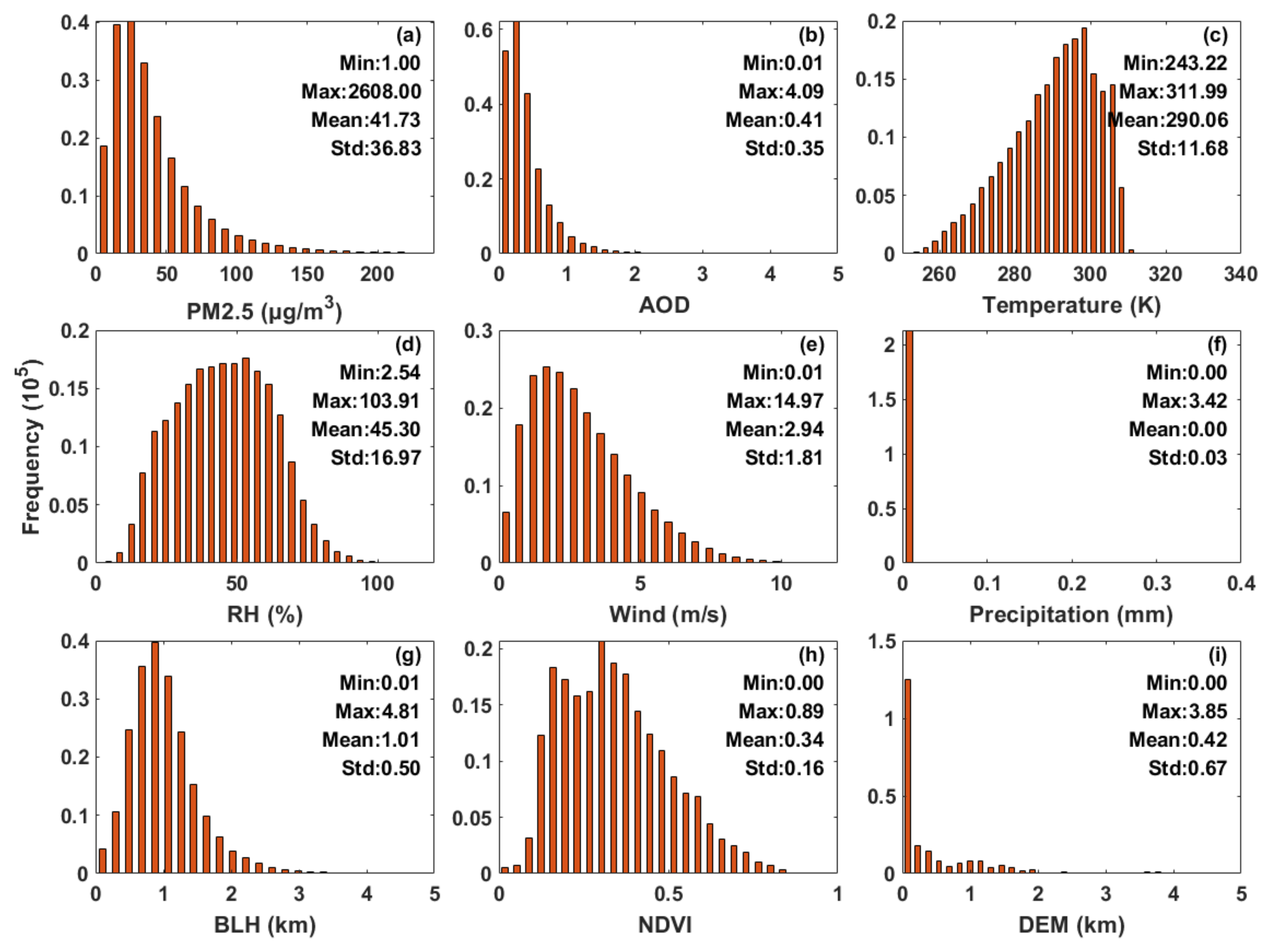
4.1.2. Statistical Analysis of the Datasets

The spatial and temporal resolution of different factors is unified to 750 m and 1 day by the linear interpolation method, respectively. After screening for abnormal data, a total of 215,893 matched data are obtained. The data are statistically analyzed, and their maximum, minimum, mean, and standard deviation are calculated. The statistical results are shown in Figure 5.

4.2. Model Evaluation and Comparison

The bagged-tree model is applied in this study; data numbering 215,893 are matched through 1591 stations, and each datum contains 13 attributes, including time, longitude, latitude, temperature, relative humidity, etc. Parameter debugging is also very important in the process of model training. Combined with the data volume and feature number, the minimum leaf size is set to 8 and the number of Learning Cycles is set to 30 in the bagged-tree model.

The performance of the STBT model is evaluated by using R², RMSE, and MAE, as shown in Figure 6. Both station-based and sample-based 10-CV method is adopted to determine whether overfitting occurs. The comparisons of the proposed STBT model and two traditional models (MLR and LME) are also Figure 6. Two kinds of 10-CV methods were adopted to verify the performance of these models. Firstly, 90% samples from the 215,893 data were randomly selected to train the STBT model, and the remaining 10% was regarded as validation samples. Secondly, considering the wide distribution of measured sites, 90% of 1591 sites are randomly selected to train the model, and the remaining 10% sites are used as verification, which can adequately reveal the prediction ability of the model in different spatial domains.

Figure 6a,d demonstrate that the MLR model exhibited low performance with site-based (sample-based) 10-CV: R² of 0.38 (0.38), the corresponding MAE is 18.18 (18.15) μg/m³, and RMSE is 29.10 (29.06) μg/m³. The complex relationship between PM_2.5 and AOD is difficult to express by a simple linear relationship. Additionally, the LME model also performed moderately well with site-based (sample-based) 10-CV: R² of 0.53 (0.52), the corresponding MAE is 15.43 (15.43) μg/m³, and RMSE is 25.33 (25.41) μg/m³ in Figure 6b,e. It is gratifying that the STBT model performs well with site-based (sample-based) 10-CV: R² value of 0.81 (0.84), the corresponding the MAE is 8.93 (8.77) μg/m³, and RMSE is 16.37 (15.14) μg/m³, as shown in Figure 6c,f. The similar verification results between site-based and sample-based 10-CV method indicate that the proposed STBT model has good prediction ability over the regions without measurements and could effectively avoid overfitting by considering spatial and temporal heterogeneity. Compared with the two traditional MLR and LME models, the R² of the proposed STBT model is higher by 121.05% and 61.54%, respectively, its RMSE is lower by 41.91% and 40.42%, respectively, and its MAE is lower by 51.69% and 43.17%, respectively. Thus, compared with other models, the STBT model shows greatly improved performance for mapping regional PM_2.5 concentrations.

Surface PM_2.5 concentrations measured by sites and estimated by the STBT model are plotted in Figure 7. The bias between estimations and measurements from during the study period (from 1 January to 31 December 2018) is plotted in the same figure. The annual average bias between the estimated and measured PM_2.5 concentration is 7.16 μg/m³. The estimated results match the measured values well, especially in summer.

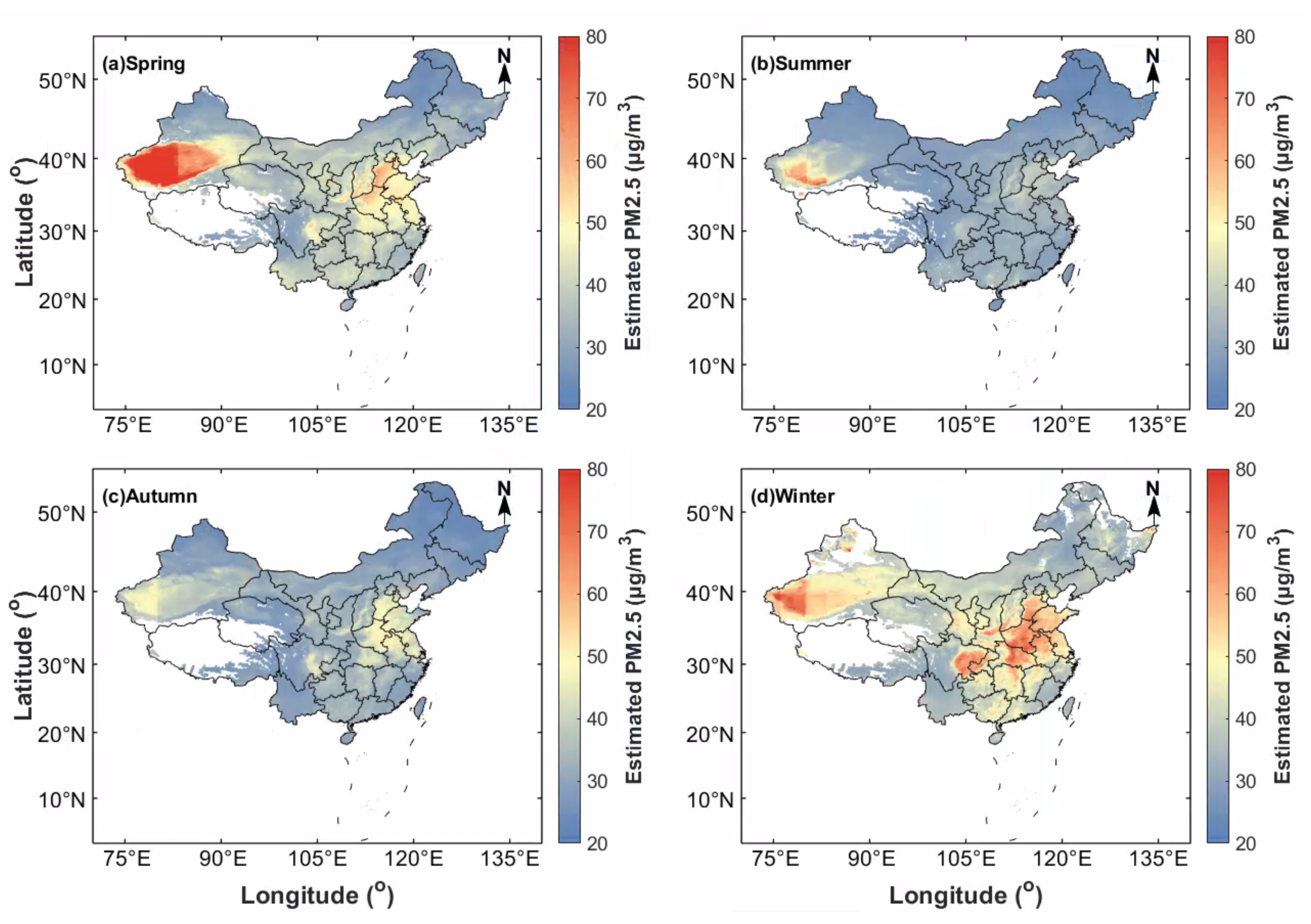
4.3. Spatial Distributions of Surface PM_2.5 Levels

Figure 8 shows the seasonal average PM_2.5 levels estimated by the STBT model across China. These subfigures reveal significant seasonal changes in the distribution of surface PM_2.5 levels. Among the four seasons, winter demonstrates the greatest levels of pollution, with an average PM_2.5 value of 44 μg/m³. By contrast, summer shows the lowest levels of pollution, with an average PM_2.5 value of 31 μg/m³. This significant seasonal change is strongly correlated with anthropogenic emissions [35,36,37,38]. A mass of particulate matter produced by burning fossil fuels and biomass promote the high polluted levels in winter [39,40]. Adverse weather conditions during cold periods could promote the accumulation of air pollutants over a certain region [41]. The low pollution in summer may be related to the less fossil fuel and biomass burning in this season. Moreover, clean marine air mass, intense atmospheric convection, and sufficient wet deposition of aerosols can significantly reduce pollution levels during the Asian summer monsoon [42]. Ground PM_2.5 concentrations also show distinct spatial inconsistency. Low seasonal PM_2.5 levels exist in the eastern coastal area. By contrast, the seasonal average PM_2.5 levels over the Beijing–Tianjin–Hebei and Xinjiang regions are high, likely because of regional industrial development or adverse terrain accumulate of air pollutants. Moreover, the performance of the STBT model in the western region may be influenced by the sparse distribution of measured stations in these regions. Furthermore, the lifetime of PM_2.5 in the atmosphere can be up to 6 days, and during those days the particles can travel up to 3000 km. The wind erosion effect leads to the very high concentration of PM_2.5 in northwestern China [43], which transports sand dust from Taklamakan Desert to adjacent areas.

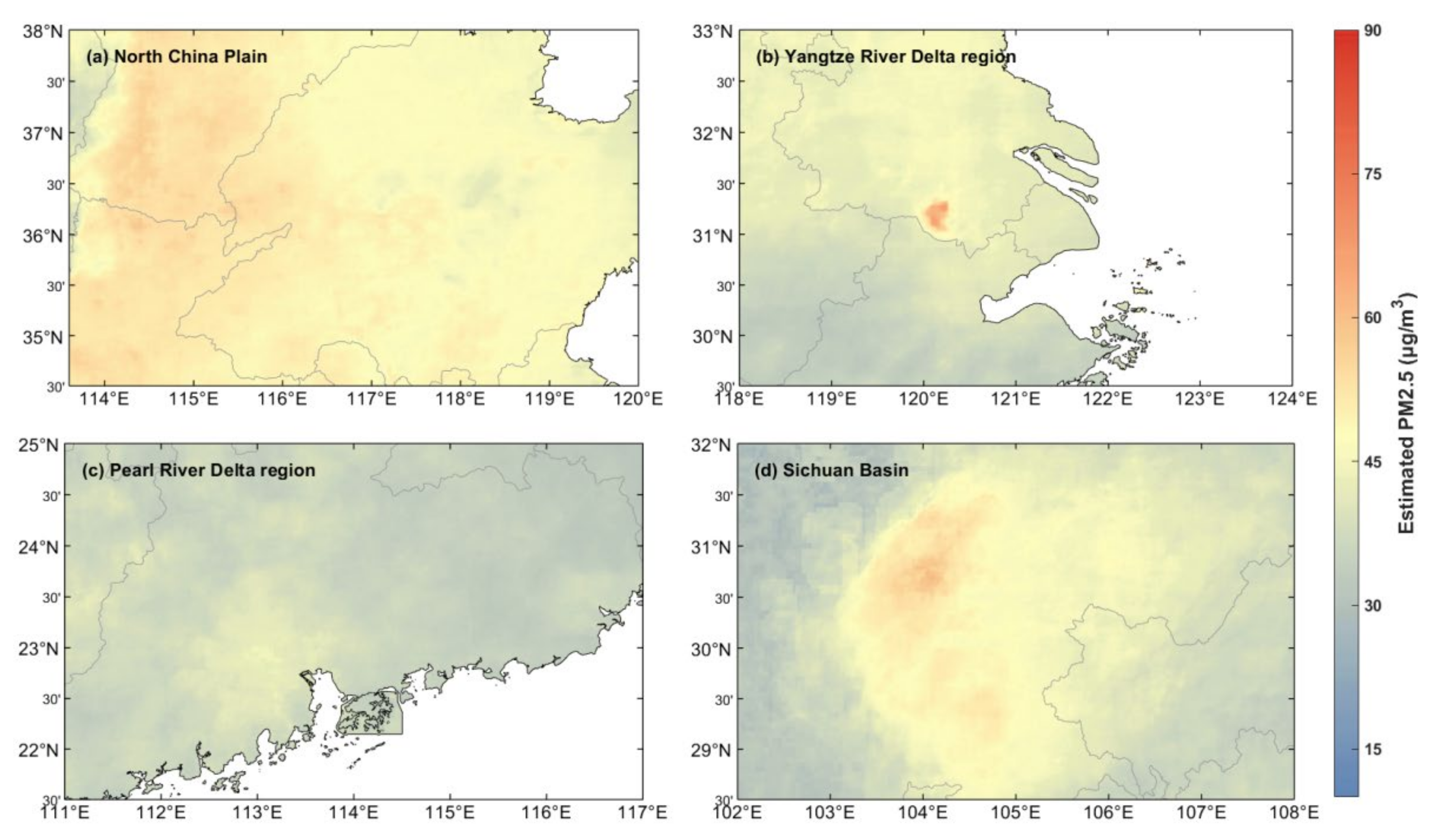
4.4. Regional PM_2.5 Concentrations

Four typical polluted regions are selected, including the Yangtze River Delta region, the North China Plain, the Sichuan Basin and the Pearl River Delta region. As shown in Figure 9, the North China Plain remains the most polluted area, due to many anthropogenic emission sources, adverse topographic conditions, and other factors [44]. The Pearl River Delta has the lowest polluted levels among the four regions, because the monsoon on the east coast disperses fine particles. The concentration of fine particles in Sichuan Basin is also relatively high, which is mainly due to the closed topography, which results in pollutant accumulation [45].

5. Conclusions

The spatiotemporal distribution of surface PM_2.5 levels across China are mapped by a STBT model using fused AOD data collected in 2018 in this study. The main conclusions follow:

(1)

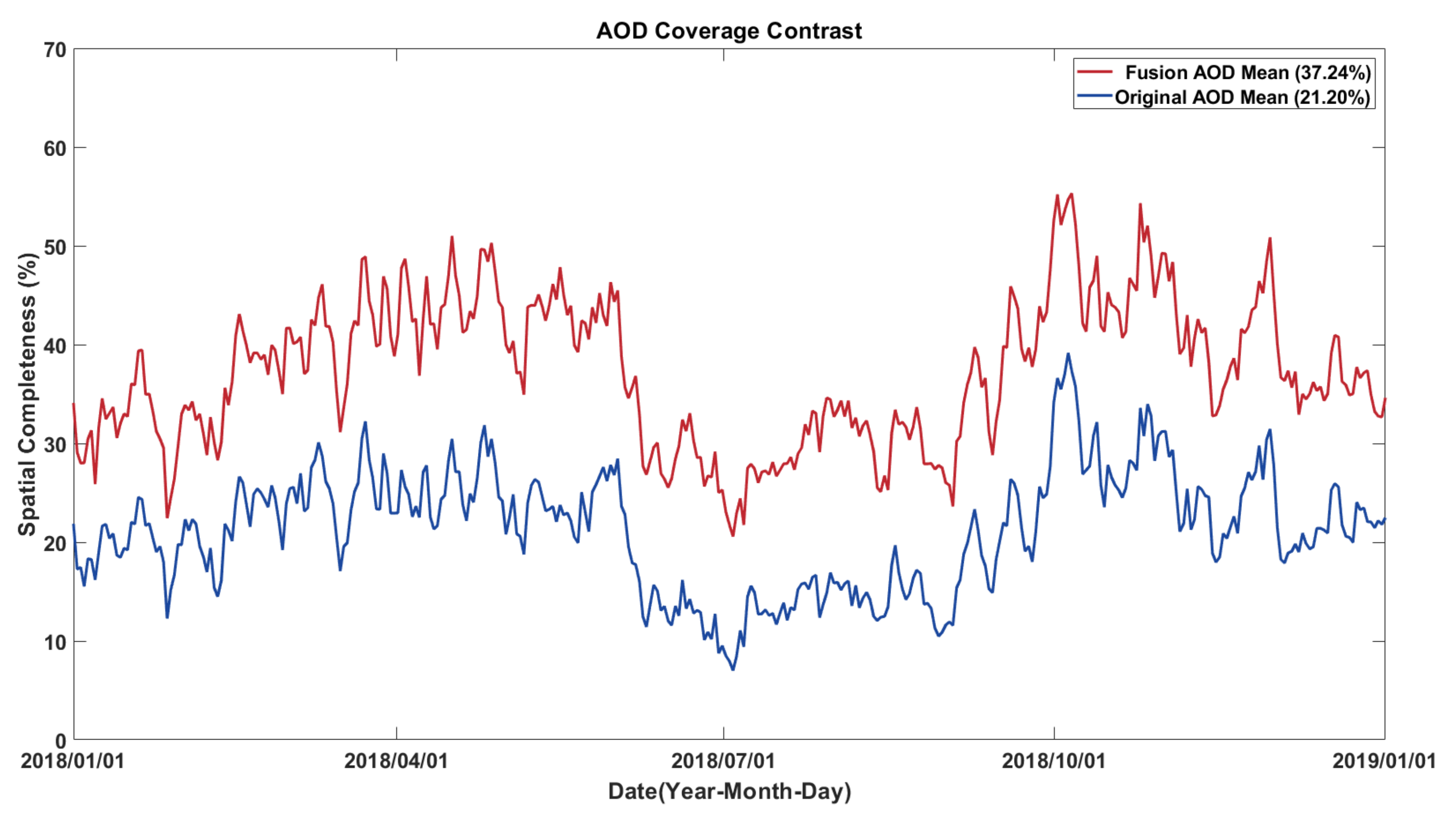
Compared with the average coverage of the original MAIAC AOD (21.20%), the coverage of the fused AOD reaches 37.24% by using an adaptive threshold algorithm of auxiliary pixels.

(2)

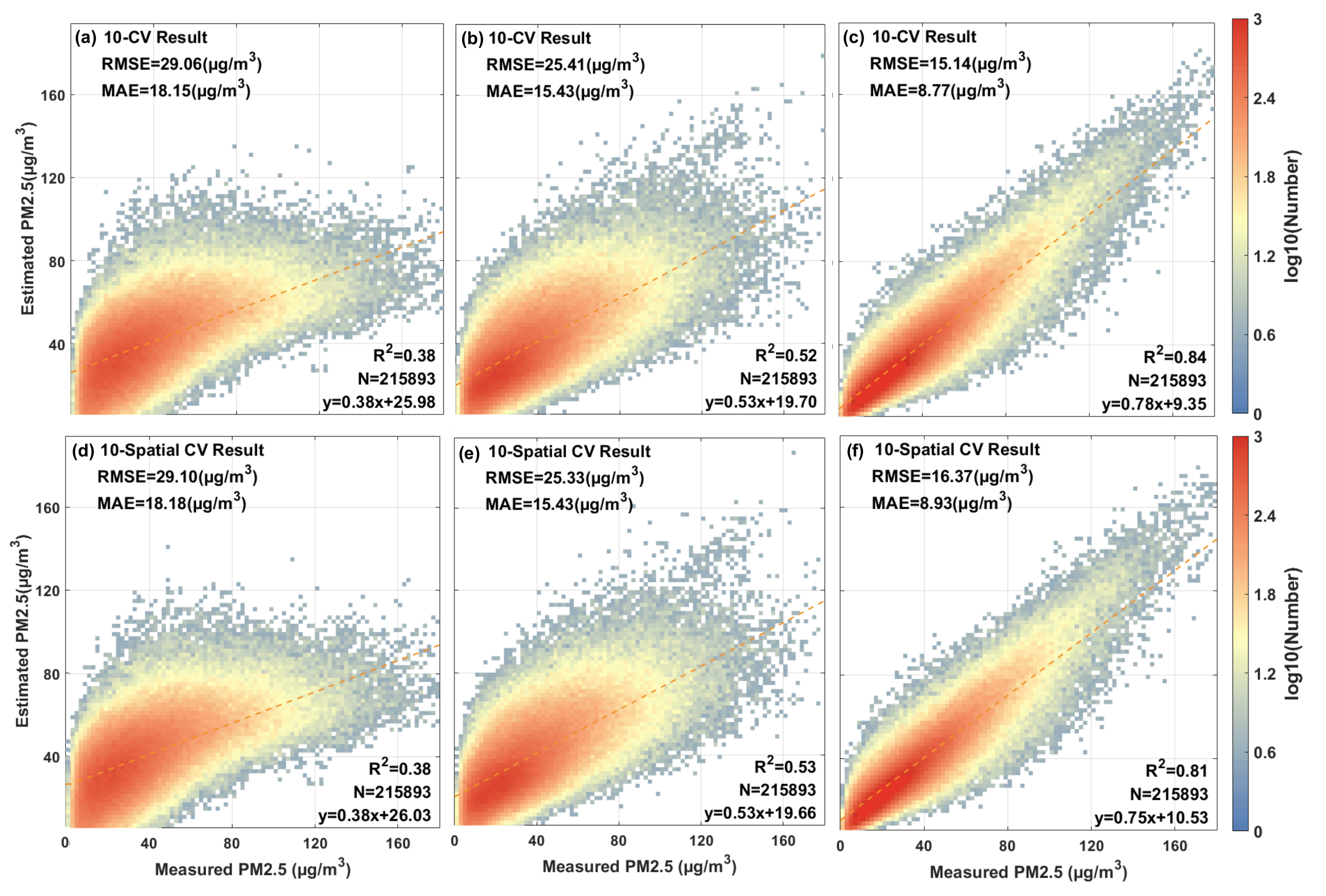
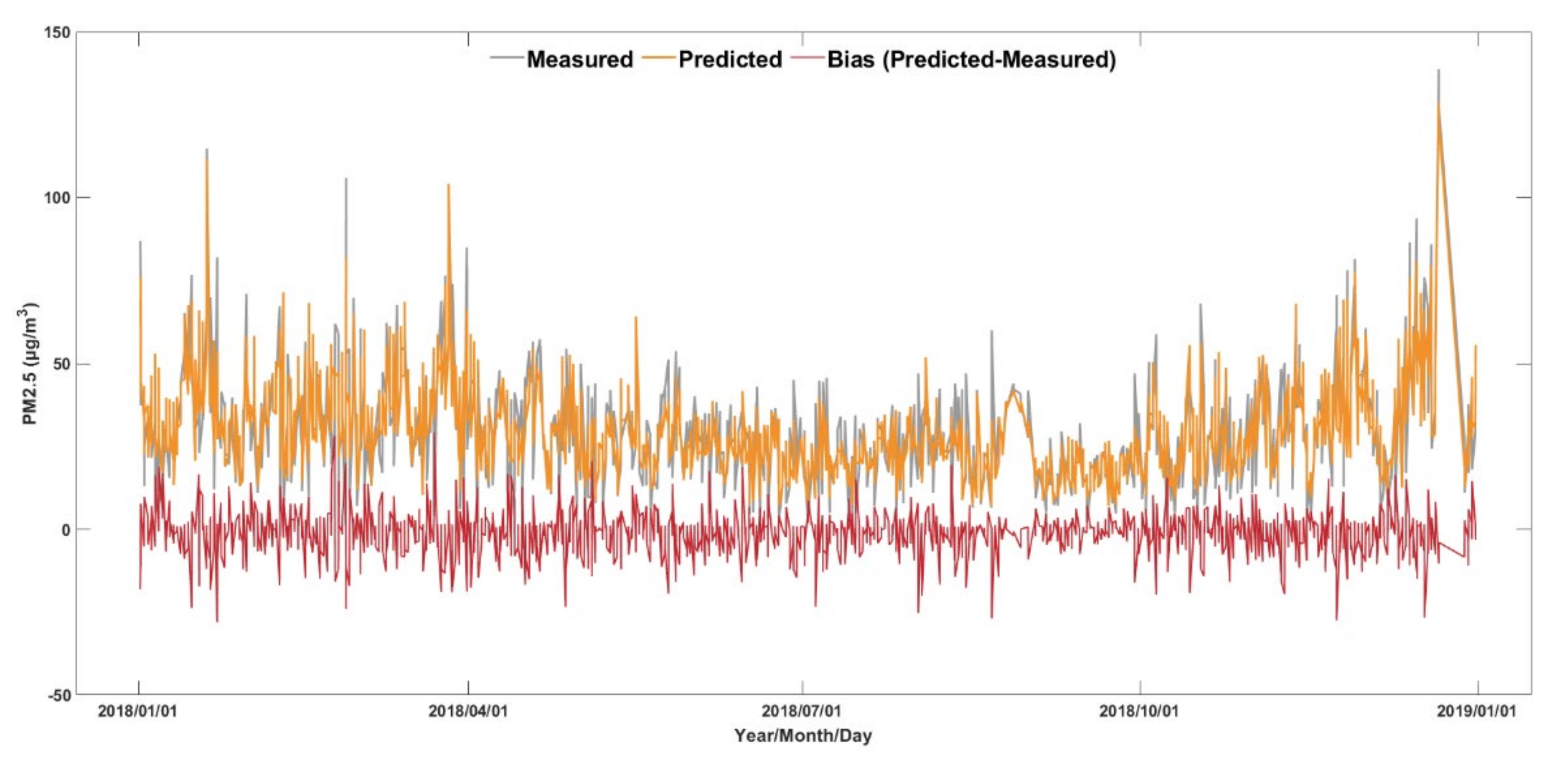
Compared with traditional MLR (R² = 0.38, MAE = 18.15 μg/m³, RMSE = 29.06 μg/m³) and LME (R² = 0.52, MAE = 15.43 μg/m³, RMSE = 25.41 μg/m³) models, the STBT model can map regional PM_2.5 concentrations with a higher R² (0.84), lower MAE (8.77 μg/m³⁾, and RMSE (15.14 μg/m³), based on sample-based 10-fold CV.

(3)

Seasonally spatial distributions of surface PM_2.5 levels estimated by the STBT model display the significant seasonal changes. Among the seasons, summer reveals the lowest pollution levels, followed by spring and autumn. Winter shows the highest pollution levels. In terms of spatial distribution, the pollution in the Beijing–Tianjin–Hebei and Xinjiang regions is high while that in the southeast coastal region is low.

The stability and performance of the STBT model is improved by considering the spatiotemporal heterogeneity of different modeling factors. In future work, our research team aims to improve models with better performance for regional PM_2.5 mapping.

References

1. Jin, M.; Yang, H.W.; Tao, A.L.; Wei, J.F. Evolution of the protease-activated receptor family in vertebrates. Int. J. Mol. Med. 2016, 37, 593–602. [Google Scholar] [CrossRef] [PubMed] [Green Version]
2. Di, Q.; Kloog, I.; Koutrakis, P.; Lyapustin, A.; Wang, Y.; Schwartz, J. Assessing PM2.5 Exposures with High Spatiotemporal Resolution across the Continental United States. Env. Sci. Technol. 2016, 50, 4712–4721. [Google Scholar] [CrossRef] [PubMed] [Green Version]
3. Ailshire, J.; Karraker, A.; Clarke, P. Neighborhood social stressors, fine particulate matter air pollution, and cognitive function among older U.S. adults. Soc. Sci. Med. 2017, 172, 56–63. [Google Scholar] [CrossRef] [Green Version]
4. Lee, M.; Schwartz, J.; Wang, Y.; Dominici, F.; Zanobetti, A. Long-term effect of fine particulate matter on hospitalization with dementia. Environ. Pollut. 2019, 254, 112926. [Google Scholar] [CrossRef]
5. Chen, H.; Kwong, J.C.; Copes, R.; Tu, K.; Villeneuve, P.J.; van Donkelaar, A.; Hystad, P.; Martin, R.V.; Murray, B.J.; Jessiman, B.; et al. Living near major roads and the incidence of dementia, Parkinson’s disease, and multiple sclerosis: A population-based cohort study. Lancet 2017, 389, 718–726. [Google Scholar] [CrossRef]
6. Di, Q.; Amini, H.; Shi, L.; Kloog, I.; Silvern, R.; Kelly, J.; Sabath, M.B.; Choirat, C.; Koutrakis, P.; Lyapustin, A.; et al. An ensemble-based model of PM2.5 concentration across the contiguous United States with high spatiotemporal resolution. Environ. Int. 2019, 130, 104909. [Google Scholar] [CrossRef]
7. Huang, K.; Xiao, Q.; Meng, X.; Geng, G.; Wang, Y.; Lyapustin, A.; Gu, D.; Liu, Y. Predicting monthly high-resolution PM2.5 concentrations with random forest model in the North China Plain. Env. Pollut. 2018, 242, 675–683. [Google Scholar] [CrossRef]
8. Dubovik, O.; Smirnov, A.; Holben, B.N.; King, M.D.; Kaufman, Y.J.; Eck, T.F.; Slutsker, I. Accuracy assessments of aerosol optical properties retrieved from Aerosol Robotic Network (AERONET) Sun and sky radiance measurements. J. Geophys. Res. Atmos. 2000, 105, 9791–9806. [Google Scholar] [CrossRef] [Green Version]
9. Chatterjee, A.; Michalak, A.M.; Kahn, R.A.; Paradise, S.R.; Braverman, A.J.; Miller, C.E. A geostatistical data fusion technique for merging remote sensing and ground-based observations of aerosol optical thickness. J. Geophys. Res. Space Phys. 2010, 115, 115. [Google Scholar] [CrossRef] [Green Version]
10. Guo, J.-P.; Zhang, X.-Y.; Che, H.-Z.; Gong, S.-L.; An, X.; Cao, C.-X.; Guang, J.; Zhang, H.; Wang, Y.-Q.; Zhang, X.-C.; et al. Correlation between PM concentrations and aerosol optical depth in eastern China. Atmos. Environ. 2009, 43, 5876–5886. [Google Scholar] [CrossRef]
11. Engel-Cox, J.A.; Holloman, C.H.; Coutant, B.W.; Hoff, R.M. Qualitative and quantitative evaluation of MODIS satellite sensor data for regional and urban scale air quality. Atmos. Environ. 2004, 38, 2495–2509. [Google Scholar] [CrossRef]
12. Xie, Y.; Wang, Y.; Zhang, K.; Dong, W.; Lv, B.; Bai, Y. Daily Estimation of Ground-Level PM2.5 Concentrations over Beijing Using 3 km Resolution MODIS AOD. Env. Sci Technol. 2015, 49, 12280–12288. [Google Scholar] [CrossRef] [Green Version]
13. Wei, J.; Li, Z.; Huang, W.; Xue, W.; Song, Y. Improved 1-km-Resolution PM2.5 Estimates across China Using the Space-Time Extremely Randomized Trees. Atmos. Chem. Phys. Discuss. 2019. [Google Scholar] [CrossRef] [Green Version]
14. Sun, T.M.; Chang, Y.H.; Chang, K.E.; Lin, T.H. Using radiance of cloud shadow for retrieve Investigation of AOD retrieval with Himawari-8 satellite data. In Proceedings of the Egu General Assembly Conference, Vienna, Austria, 17–22 April 2016. [Google Scholar]
15. Wang, W.; He, J.; Miao, Z.; Du, L. Space–Time Linear Mixed-Effects (STLME) Model for Mapping Hourly Fine Particulate Loadings in the Beijing–Tianjin–Hebei Region, China. J. Clean. Prod. 2021, 292, 125993. [Google Scholar] [CrossRef]
16. Lyapustin, A.; Wang, Y.; Korkin, S.; Huang, D. Collection 6 MAIAC algorithm. Atmos. Meas. Tech. 2018, 11, 5741–5765. [Google Scholar] [CrossRef] [Green Version]
17. Lyapustin, A.; Wang, Y.; LaszloI, I.; Korkin, S. Improved cloud and snow screening in MAIAC aerosol retrievals using spectral and spatial analysis. Atmos. Meas. Tech. 2012, 5, 843–850. [Google Scholar] [CrossRef] [Green Version]
18. Liu, H.; Remer, M.A.; Huang, J. Preliminary evaluation of S-NPP VIIRS aerosol optical thickness. J. Geophys. Res. Atmos. 2014, 119, 3942–3962. [Google Scholar] [CrossRef]
19. Jackson, J.M.; Liu, H.; Laszlo, I.; Kondragunta, S.; Remer, L.A.; Huang, J.; Huang, H.C. Suomi-NPP VIIRS aerosol algorithms and data products. J. Geophys. Res. Atmos. 2013, 118, 12673–12689. [Google Scholar] [CrossRef]
20. Zhang, Y.; Li, Z. Remote sensing of atmospheric fine particulate matter (PM2.5) mass concentration near the ground from satellite observation. Remote Sens. Environ. 2015, 160, 252–262. [Google Scholar] [CrossRef]
21. Li, T.; Shen, H.; Yuan, Q.; Zhang, X.; Zhang, L. Estimating Ground-Level PM2.5 by Fusing Satellite and Station Observations: A Geo-Intelligent Deep Learning Approach. Geophys. Res. Lett. 2017. [Google Scholar] [CrossRef] [Green Version]
22. Yu, W.; Liu, Y.; Ma, Z. Improving satellite-based PM2.5 estimates in China using Gaussian processes modeling in a Bayesian hierarchical setting. Sci. Rep. 2017, 7, 1–9. [Google Scholar] [CrossRef] [Green Version]
23. Ma, Z.; Hu, X.; Huang, L.; Bi, J.; Liu, Y. Estimating Ground-Level PM2.5 in China Using Satellite Remote Sensing. Env. Sci. Technol. 2014, 48, 7436–7444. [Google Scholar] [CrossRef]
24. Chen, G.; Li, S.; Knibbs, L.D.; Hamm, N.A.S.; Cao, W.; Li, T.; Guo, J.; Ren, H.; Abramson, M.J.; Guo, Y. A machine learning method to estimate PM2.5 concentrations across China with remote sensing, meteorological and land use information. Sci. Total Env. 2018, 636, 52–60. [Google Scholar] [CrossRef] [PubMed]
25. Chen, Y.; Wu, S.; Wang, Y.; Zhang, F.; Du, Z. Satellite-Based Mapping of High-Resolution Ground-Level PM2.5 with VIIRS IP AOD in China through Spatially Neural Network Weighted Regression. Remote Sens. 2021, 13, 1979. [Google Scholar] [CrossRef]
26. Mhawish, A.; Banerjee, T.; Sorek-Hamer, M.; Lyapustin, A.; Broday, D.M.; Chatfield, R. Comparison and evaluation of MODIS Multi-Angle Implementation of Atmospheric Correction (MAIAC) aerosol product over South Asia. Remote Sens. Environ. 2019, 224, 12–28. [Google Scholar] [CrossRef]
27. Meng, F.; Cao, C.; Shao, X. Spatio-temporal variability of Suomi-NPP VIIRS-derived aerosol optical thickness over China in 2013. Remote Sens. Environ. 2015, 163, 61–69. [Google Scholar] [CrossRef]
28. Yao, F.; Si, M.; Li, W.; Wu, J. A multidimensional comparison between MODIS and VIIRS AOD in estimating ground-level PM2.5 concentrations over a heavily polluted region in China. Sci. Total. Environ. 2018, 618, 819–828. [Google Scholar] [CrossRef] [PubMed]
29. Karagiannidis, A.; Poupkou, A.; Giannaros, T.; Giannaros, C.; Melas, D.; Argiriou, A. The Air Quality of a Mediterranean Urban Environment Area and Its Relation to Major Meteorological Parameters. Water Air Soil Pollut. 2015, 226, 2239. [Google Scholar] [CrossRef]
30. Zhang, T.; Chao, Z.; Wei, G.; Wang, L.; Zhu, Z. Improving spatial coverage for Aqua MODIS AOD using NDVI-based multi-temporal regression analysis. Remote Sens. 2017, 9, 340. [Google Scholar] [CrossRef] [Green Version]
31. Yuan, W.A. Large-scale MODIS AOD products recovery: Spatial-temporal hybrid fusion considering aerosol variation mitigation. ISPRS J. Photogramm. Remote Sens. 2019, 157, 1–12. [Google Scholar]
32. Wang, W.; Mao, F.; Pan, Z.; Du, L.; Gong, W. Validation of VIIRS AOD through a Comparison with a Sun Photometer and MODIS AODs over Wuhan. Remote Sens. 2017, 9. [Google Scholar] [CrossRef] [Green Version]
33. Margineantu, D.D.; Dietterich, T.G. Improved Class Probability estimates from Decision Tree Models. Nonlinear Estim. Classif. 2003, 171, 173–188. [Google Scholar]
34. Banfield, R.E.; Hall, L.O.; Bowyer, K.W.; Kegelmeyer, W.P. A comparison of decision tree ensemble creation techniques. IEEE Trans. pattern Anal. Mach. Intell. 2007, 29, 173–180. [Google Scholar] [CrossRef]
35. Rodriguez, S.; Querol, X.; Alastuey, A.; Viana, M.-M.; Alarcón, M.; Mantilla, E.; Ruiz, C.R. Comparative PM10–PM2.5 source contribution study at rural, urban and industrial sites during PM episodes in Eastern Spain. Sci. Total Environ. 2004, 328, 95–113. [Google Scholar] [CrossRef]
36. Zhang, Y.L.; Cao, F. Fine particulate matter (PM 2.5) in China at a city level. Sci Rep. 2015, 5, 14884. [Google Scholar] [CrossRef] [Green Version]
37. Wang, W.; Mao, F.; Du, L.; Pan, Z.; Gong, W.; Fang, S. Deriving Hourly PM2.5 Concentrations from Himawari-8 AODs over Beijing–Tianjin–Hebei in China. Remote Sens. 2017, 9, 858. [Google Scholar] [CrossRef] [Green Version]
38. Wang, W.; Mao, F.; Zou, B.; Guo, J.; Wu, L.; Pan, Z.; Zang, L. Two-stage model for estimating the spatiotemporal distribution of hourly PM1. 0 concentrations over central and east China. Sci. Total Environ. 2019, 675, 658–666. [Google Scholar] [CrossRef]
39. Nava, S.; Prati, P.; Lucarelli, F.; Mandò, P.A.; Zucchiatti, A. Source Apportionment in the Town of La Spezia (Italy) by Continuous Aerosol Sampling and PIXE Analysis. Water Air Soil Pollut. Focus 2002, 2, 247–260. [Google Scholar] [CrossRef]
40. Rushdi, A.I.; Al-Mutlaq, K.F.; Al-Otaibi, M.; El-Mubarak, A.H.; Simoneit, B.R.T. Air quality and elemental enrichment factors of aerosol particulate matter in Riyadh City, Saudi Arabia. Arab. J. Geosci. 2013, 6, 585–599. [Google Scholar] [CrossRef]
41. Noble, C.A.; Mukerjee, S.; Gonzales, M.; Rodes, C.E.; Lawless, P.A.; Natarajan, S.; Myers, E.A.; Norris, G.A.; Smith, L.; Oezkaynak, H. Continuous measurement of fine and ultrafine particulate matter, criteria pollutants and meteorological conditions in urban El Paso, Texas. Atmos. Environ. 2003, 37, 827–840. [Google Scholar] [CrossRef]
42. Yoo, J.M.; Lee, Y.R.; Kim, D.; Jeong, M.J.; Stockwell, W.R.; Kundu, P.K.; Oh, S.M.; Shin, D.B.; Lee, S.J. Corrigendum to “New indices for wet scavenging of air pollutants (O 3,CO, NO 2, SO 2, and PM 10) by summertime rain”. Atmos. Environ. 2014, 91, 226–237. [Google Scholar] [CrossRef]
43. Jorquera, H.; Barraza, F. Source apportionment of PM and PM. in a desert region in northern Chile. Sci. Total. Environ. 2013, 444, 327–335. [Google Scholar] [CrossRef] [PubMed]
44. He, Q.; Huang, B. Satellite-based high-resolution PM2.5 estimation over the Beijing-Tianjin-Hebei region of China using an improved geographically and temporally weighted regression model. Environ. Pollut. 2018, 236, 1027–1037. [Google Scholar] [CrossRef] [PubMed]
45. He, Q.; Huang, B. Satellite-based mapping of daily high-resolution ground PM 2.5 in China via space-time regression modeling. Remote Sens. Environ. 2018, 206, 72–83. [Google Scholar] [CrossRef]
Figure 1. Distribution of PM measured sites managed by the China National Environmental Monitoring Center (CNEMC). The total number of monitoring sites is 1591.
Ijgi 10 00676 g001
Figure 2. Validation results of total data for (a) original MAIAC AOD and (b) fusion MAIAC AOD. The color bar presents counts of points. Number of samples (N), correlation coefficient (R), RMSE, and bias are given in each subplot.
Ijgi 10 00676 g002
Figure 3. Time series plot of daily coverage for original (red line) and fused (blue line) MAIAC AOD. The numbers in parentheses represent the averaged AOD coverage.
Ijgi 10 00676 g003
Figure 4. Maps of quarterly AOD coverage for original (ad) and fused (eh) MAIAC AOD. The color bar represents AOD coverage (%). Spring: March–May; Summer: June–August; Autumn: September–November; Winter: December–February.
Ijgi 10 00676 g004
Figure 5. Statistical analysis of the datasets used in this study, including PM2.5, AOD, temperature, RH, wind, precipitation, BLH, NDVI, and DEM.
Ijgi 10 00676 g005
Figure 6. Scatterplot of the sample-based (ac) and station-based (df) CV for surface PM2.5 estimations from the different models: (a,d) MLR, (b,e) LME, and (c,f) STBT model.
Ijgi 10 00676 g006
Figure 7. Time series plot of estimations from the STBT model and measurements together with bias between estimations and measurements. The abscissa represents the time of two hours before and after 12:00 local time, and the ordinate represents the average of the observed values of all stations in that hour.
Ijgi 10 00676 g007
Figure 8. Spatial distribution of seasonal PM2.5 concentrations estimated by the STBT model: (a) Spring, (b) Summer, (c) Autumn, and (d) Winter.
Ijgi 10 00676 g008
Figure 9. Annual averaged surface PM2.5 levels in 2018 for four typical polluted regions: (a) North China Plain, (b) Yangtze River Delta region, (c) Pearl River Delta region, and (d) Sichuan Basin.
Ijgi 10 00676 g009