1. Introduction
Since the emergence of modern robots in the early 1950s, robot control became a thriving field of research as interest grew [
1]. Conventional control of robotic systems, such as manipulators, is based on the kinematics and dynamics of rigid bodies that use joint-space to task-space transformations to calculate their poses [
2]. This approach leaves the controller heavily dependent on the robot’s configuration, which assumes a static arrangement of joints and links. This kinematic-model-based approach has remained the prevalent control method for over half a century [
3].
Over the past 70 years, several control approaches, such as model-approximating and model-learning, have emerged. Nevertheless, true model-free control remains a challenging problem. In our previous work, the Encoderless Robot Control [
4] and Kinematic-Free Control [
5] (which we propose to call “Kinematic-Model-Free” (KMF) Controllers) successfully controlled a robot manipulator’s end effector in task space without requiring any prior kinematic model of the robot by learning local linear models. However, these controllers only managed to control the position of a two-degrees-of-freedom (DOF) planar robot, leaving orientation control unsolved.
Orientation control imposes challenges due to the discontinuities or singularities that exist in the orientation spectrum, such as the gimbal lock in Euler angles or angle wrapping that occurs after a full rotation. Without resolving these issues, the robot will misinterpret movements when crossing the point of discontinuity or can take a longer route to reach the desired target, causing the robot to behave undesirably and inefficiently. Quaternions, discovered by Hamilton around 1844 [
6], are an extension to the complex number system and are able to represent rotations without suffering from discontinuities. Furthermore, dual quaternions (DQs), introduced by Clifford around 1873 [
7], provide a unified representation of a rigid link’s pose, both position and orientation. Linear combinations of dual quaternions are used in this research to learn a local kinematics and dynamics (what we call ‘kinodynamics’) model of the robot.
The contributions of this paper are the following: (1) the controller presented in this paper extends the state-of-the-art KMF controller to control both the position and orientation of a robot’s end effector; (2) the robot controlled is a 3-DOF robot that allows multiple orientation solutions for given target positions, scaling up from the 2-DOF robot manipulator in our previous work; (3) this paper also presents the equations for finding relative dual quaternions and for taking a weighted sum of dual quaternions, both of which are key in developing our KMF-DQ controller.
2. Related Work
In any introductory course about robotics, the first type of controller taught is the conventional controller in which a Jacobian, which is characteristic to the robot’s configuration, is populated [
8]. Robots are controlled using forward and inverse kinematics and dynamics. Most of the literature in robot control assumed that the robot’s Jacobian matrix is known. This assumption imposes many limitations [
9], which implies that the link lengths and joint offsets must be known and static. However, this assumption breaks when the robot is soft or damaged and if the robot picks up a tool, modifying its end effector [
10]. Any change in the robot’s configuration will cause the controller to fail and a new model has to be generated. Thus, conventional controllers are accurate but not flexible.
Model-based controllers use the kinematic and dynamic model of the robot [
11]. A well-known example is visual servoing [
12]. Visual servoing uses a camera to calculate the velocity of the end effector required to reach a target. The controller sends the calculated velocity commands to a conventional velocity controller to move the robot [
4]. However, as with all model-based controllers, any change to the robot’s kinematics will result in undesirable behaviour and failure. Recent advances in robot control include approximating a model of the robot. Researchers in [
13,
14,
15] controlled a deformable manipulator by approximating a Jacobian. Some researchers addressed the issue of controlling a dynamically undefined robot by identifying and estimating the system’s dynamic parameters, which were then used alongside conventional controllers to control the robot [
16].
Other controllers start with no prior knowledge about the robot’s kinematic/dynamic properties and try to learn a model for controlling the robot. Examples include motor babbling [
17] and reinforcement learning [
18], which uses machine learning techniques to control a robot. However, all of these approaches rely on joint position feedback (through encoders) for estimating the robot’s kinematic pose.
The model-learning approach presented in our preliminary work in [
4,
5] are KMF controllers because they start with no prior knowledge about the robot’s configuration and learn a model without requiring kinematic information about the robot’s joint position during control. Instead, these approaches use exteroception, similar to visual servoing to learn a local linear model that is used to drive the end effector towards a reference target. The controller starts by recording end effector displacements by sending random actuation primitives in the form of square torque waveforms using a camera. The recorded information about the joint torques and their resulting end-effector displacements are then used to calculate a new primitive that will move the end effector towards a given target. The state-of-the-art KMF controller only addressed position control of a 2-DOF planar robot, leaving orientation control and control of manipulators of higher degrees-of-freedom unsolved.
3. Mathematical Background
3.1. Quaternions
Quaternions are an extension to the complex number system used to represent rotations, first described by Hamilton around 1844 [
6]. A quaternion
is the sum of a scalar
s and a vector
:
where
i,
j,
k are unit vectors pointing along the x-,y-,z-axes. The addition and subtraction of quaternions are element-wise:
The conjugate of a quaternion
is defined as:
from which the norm of a quaternion can be calculated as
. A quaternion
is unit when
or simply
. The
operator maps the elements of a quaternion
to a 4-dimensional vector
. A detailed examination of quaternions can be found in [
19].
3.2. Dual Quaternions
Dual quaternions, introduced by Clifford [
7], are an extension to the dual number system used to represent rigid transformations by unifying rotational and translational information into a single mathematical object. A dual quaternion
is the sum of two quaternions:
where
is the real part and
is the dual part. The dual element
is nilpotent,
. The addition and subtraction of two dual quaternions are performed separately on the real and dual parts:
The conjugate of a dual quaternion is . The norm of a dual quaternion is defined as . A dual quaternion is unit when the real part is unit and is perpendicular to the dual part, and or simply when and . The operator maps the elements of a dual quaternion to an 8-dimensional vector .
3.3. Rigid Transformation
A rigid transformation can be represented using a dual quaternion:
where
is the rotation quaternion and
is the translation quaternion [
20]. From a unit dual quaternion
, the rotation and translation quaternions are derived as:
and
, where
r is the rotation quaternion and
t is the translation quaternion. For the translation quaternion, the scalar part is always zero,
. The dual quaternion transformation represents a pure rotation when the dual part is zero,
.
3.4. Interpolation
Interpolation between two 3D rotations represented by two quaternions is achieved using Spherical Linear Interpolation (SLERP) which, was introduced by Shoemake in 1985 [
21]. This method of interpolation is popular because it has the following desirable properties: constant speed, shortest path, and coordinate system invariant [
22]. Let
denote an interpolation between
and
, where
. The interpolated quaternion is then
Screw Linear Interpolation (ScLERP) is a generalization of SLERP that extends it to interpolate between dual quaternions and is defined similarly,
where
.
3.5. Relative Dual Quaternions
The relative rotational displacement,
, between two quaternions,
and
, can be easily found as
. Finding the relative dual quaternion,
, between two dual quaternions,
and
, is not as straightforward. The dual quaternions are split into their rotational and translational quaternions and then recombined after calculating the relative rotation and translation as follows:
Note that must be a unit dual quaternion and normalized if not.
3.6. Dual Quaternion Distance
The KMF-DQ approach requires distance metrics between two dual quaternions, which will provide a measure of how close the end effector is to the target pose that reduces to zero as the end effector approaches the target. The
and
functions are used to find the distance between two dual quaternions as follows,
where
is the null dual quaternion. This measure of distance satisfies the following three properties:
Although unifying both translational and rotational distances into a single distance metrics can be an ambiguous measure of distance between poses, we can still see that as , which is suitable for our control purposes; to know when the end effector has reached the target and to end execution.
3.7. Dual Quaternion Scaling
Vectors are scaled by multiplying them by a constant. To develop a similar scaling of dual quaternions by some factor
c, they must be broken into their translational and rotational quaternions and then recombined after scaling as follows:
where the exponential of some quaternion
. The definitions of
and
can be found in [
23]. Note that
must be a unit dual quaternion and normalized if not. For example,
would result in a dual quaternion composed of twice the rotation and translation.
3.8. Dual Quaternion Linear Combination
To find a weighted sum of dual quaternions
using weights
, we decompose the dual quaternions into their rotational quaternions,
, and translational quaternions,
. The weighted sum of the rotational quaternions is as follows:
which can be written more compactly:
The weighted sum of the translational quaternions is calculated as follows:
or more compactly:
As a result, the weighted sum of the dual quaternions is computed as:
3.9. Dual Quaternion Regression
Regression can be seen as the inverse problem of calculating the weighted sum. The functions
and
are used to find the regression coefficients,
, of the dual quaternions
that yield some desired dual quaternion
:
where
which can be optimized using some optimization algorithm. In our implementation of the KMF-DQ, MATLAB’s FMINCON optimization algorithm was used.
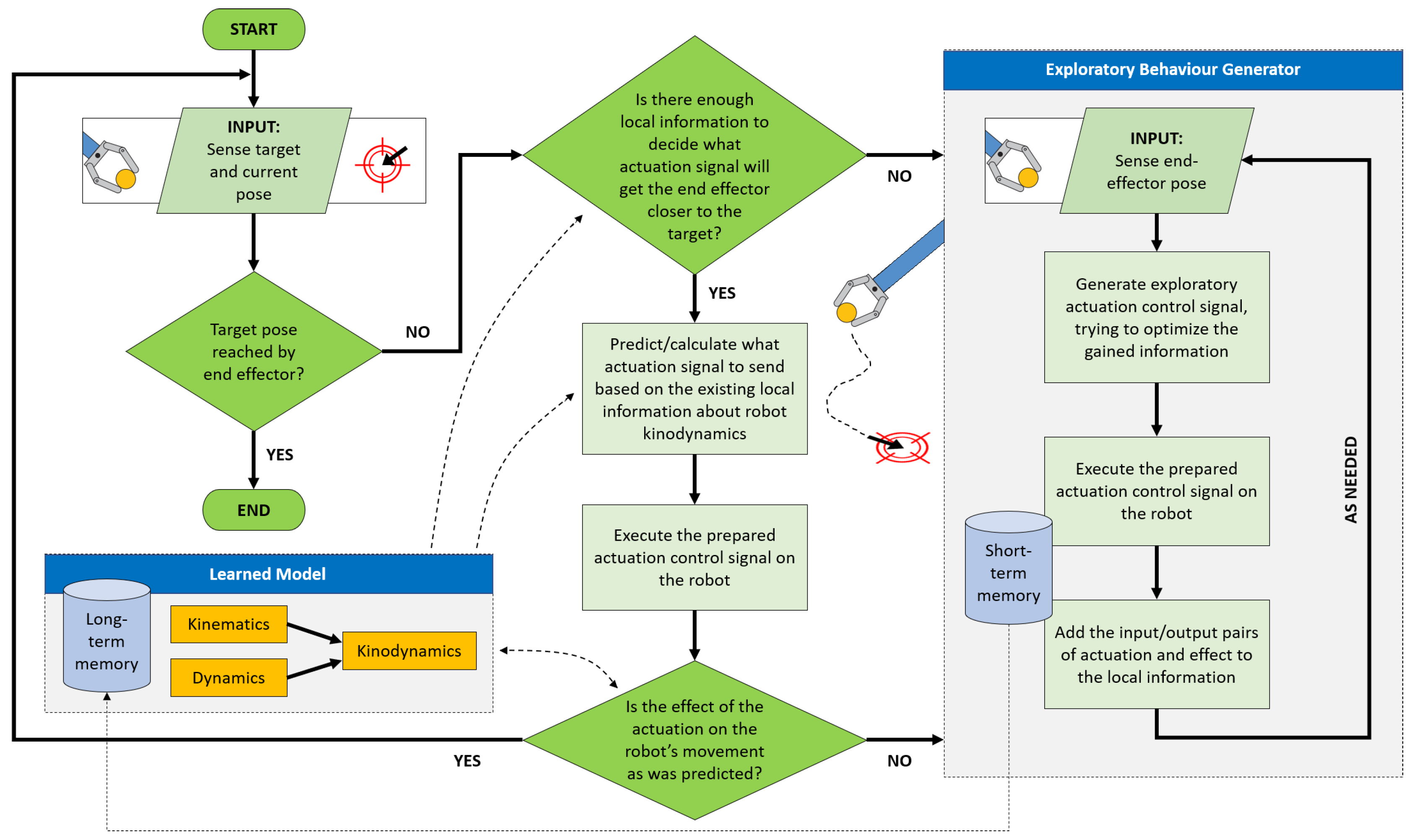
4. Proposed Approach
A high-level flowchart of the KMF-DQ controller is shown in
Figure 1. At the core of the idea lies the assumption that it is possible to obtain information about the local kinodynamics of the robotic manipulator, which is gathered by generating pseudo-random actuation control signals and observing their effects on the robot’s end effector. The torque actuation signals are square waves, as shown in
Figure 2. The actuation primitive produces a torque signal
sent to each actuator in the robot and is defined as follows:
As shown in the flowchart, if the end effector reached the target, the controller ends the execution. Otherwise, the end effector is to reach a set of intermediate targets
that lead to the final desired target pose
in discrete steps. These intermediate targets are found using ScLERP interpolation between the end effector’s current pose,
, and the desired target pose,
. At each step, the controller tries to estimate an actuation primitive,
, to move the end effector towards the desired goal pose:
where
is the magnitude of the actuation primitive of actuator
j. After each actuation, the end effector displacement is recorded as an observation, which is calculated using the
function. The nearest
k observation dual quaternions form the observation vector:
These dual quaternions contain the rotational and translational displacements caused by the executed actuation primitives. The actuation primitives corresponding to these observations form the actuation matrix:
The desired actuation primitive,
, is assumed to be a linear combination of the
k nearest actuation primitives:
where
is a set of unknown weights. These weights are found by solving the local regression of the observation vector:
With the weights, the desired actuation is then computed using Equation (
13). After the completion of each finite actuation, the resulting effect on the end effector’s state is compared with the anticipated effect. If the difference is significant, this means that the local linear model approximation of the local kinodynamics was not known precisely enough, which will trigger a new exploratory phase as shown in
Figure 1. The controller escapes the exploratory phase once it has done a set number of explorations. Lastly, the algorithm terminates when
, where
is the termination accuracy.
We stress that this approach does not require any joint angle information or prior knowledge about the robot’s kinematics and dynamics. As such, this controller is able to adapt to kinematic and dynamic changes in the robot such as changes to robot links’ sizes and extensions to the end effector. However, since the KMF-DQ controller is a discrete controller and is not based on an accurate model, the KMF-DQ controller can be used to control the robot where flexibility is favoured over precision and speed. As with other complex models such as [
24,
25], the convergence of the KMF-DQ controller is not guaranteed.
5. Simulation and Results
A dynamic simulation of a 3-DOF robot was performed using MATLAB’s Robotics Toolbox [
26] and DQ Robotics Toolbox [
26]. The kinematic and dynamic specifications of the robot used for the experiments are shown in
Table 1.
The information in
Table 1 is not given to the KMF-DQ controller. The controller was implemented as described in
Section 4 using
nearest neighbours comprising of actuation primitives and their corresponding observations. Since this experiment was conducted in simulation, there was no need to use a camera to obtain the end-effector’s state. Instead, this was achieved internally from the simulator. We note that gravity is neglected in the simulation to keep the focus on simultaneous position and orientation control, deferring gravity compensation until future research.
The experiment involves a set of reaching tasks. The controller must move the robot’s end effector to four target poses, drawing a polygon in 3D space. The position and orientation of the four target poses are listed in
Table 2. The starting position of the robot was (−0.85059, 1.2148, −0.12941) and orientation was (−1.5708, 0.9599, 2.8798).
The orientations are specified here in Euler XYZ angles for simplicity. The poses were selected to be within the robot’s reachable workspace. The results are shown in
Figure 3 in all three orthogonal views. The KMF-DQ controller generates intermediate targets to follow the yellow trajectory. The robot successfully reaches all four target poses, drawing the polygon in 3D space. These results prove that the local kinodynamic information of the robot is sufficient to create a local model that can be used to actuate the end effector towards a given target. Note that the specified target poses must lie within the robot’s reachable workspace, otherwise a higher termination tolerance,
, must be set.
To demonstrate the actuation primitives generated by the controller,
Figure 4 shows the sequence of actuated primitives of the first reaching task (moving towards target 1). Since the KMF-DQ is a discrete controller, the figure shows the discrete primitives sent to the actuators. We note that as the end effector reaches the target, lower torques are sent to the actuators. The joint position of the three joints corresponding to the first reaching task is shown in
Figure 5 to demonstrate the resulting displacements in the joints.
We can see that the joint angles of the three joints vary smoothly with no sudden jerks. Furthermore,
Figure 6 shows the pose distance of the end effector to the targets using the
function. We note that the pose distance approaches zero as the end effector approaches the targets.
Although not guaranteed, the simulation demonstrated convergence to the desired targets. The controller’s robustness was measured by running the simulation 100 times, each with a random starting robot configuration and a randomly placed target pose within the robot’s reachable workspace that is achievable within 100 steps. The target poses lie within the robot’s achievable configuration space. It was found that 87% of the time, the controller successfully performed the reaching task. In the remaining 13%, the controller did not converge to solutions that actuate the robot towards the targets. These failures can occur because the optimizer gets stuck in a local minimum, which will yield inaccurate results for the weights and thus the calculated actuation primitives.
6. Conclusions
This paper presented a novel model-free controller for robot manipulation using locally weighted combinations of dual quaternions. The approach does not require any joint angle information or prior knowledge about the robot’s kinematics and dynamics. The controller works by executing random actuation primitives and perceiving their resulting effects on the end effector. These pieces of information are then used to build a local kinodynamic model. An actuation primitive is calculated using dual quaternion regression, which is executed on the robot to move the end effector towards a given target.
We presented the dual quaternion distance, relative dual quaternion, and dual quaternion regression functions used for building a local kinodynamic model. Simulation experiments were conducted in which a manipulator performed a set of reaching tasks. The simulation results show that this novel approach can reach a set of reference poses, successfully performing simultaneous position and orientation control. Furthermore, the robustness of the approach was tested by running the simulation 100 times with random target poses that lie within the robot’s reachable workspace, which are achievable by some configuration of the robot. The controller managed to successfully reach the target poses 87% of the time within 100 steps.
The proposed approach looks promising and can be used in applications where simultaneous translational and rotational reaching is required. This approach can be used for new robot designs where a model is not present and where flexibility is favoured over precision and speed. With regards to future work, scalability to higher-degrees-of-freedom robot manipulators, continuous control, and practical real-world implementation issues such as joint limits and friction remain open problems that will be investigated in future research. Also, key issues that hindered the immediate experimentation of the proposed controller to physical experiments, such as gravity compensation and friction compensation, must be tackled before the experiments are performed since the current controller does not take into account these physical phenomena.


