FloorVLoc: A Modular Approach to Floorplan Monocular Localization

Abstract

Intelligent vehicles for search and rescue, whose mission is assisting emergency personnel by visually exploring an unfamiliar building, require accurate localization. With GPS not available, and approaches relying on new infrastructure installation, artificial landmarks, or pre-constructed dense 3D maps not feasible, the question is whether there is an approach which can combine ubiquitous prior map information with a monocular camera for accurate positioning. Enter FloorVLoc—Floorplan Vision Vehicle Localization. We provide a means to integrate a monocular camera with a floorplan in a unified and modular fashion so that any monocular visual Simultaneous Localization and Mapping (SLAM) system can be seamlessly incorporated for global positioning. Using a floorplan is especially beneficial since walls are geometrically stable, the memory footprint is low, and prior map information is kept at a minimum. Furthermore, our theoretical analysis of the visual features associated with the walls shows how drift is corrected. To see this approach in action, we developed two full global positioning systems based on the core methodology introduced, operating in both Monte Carlo Localization and linear optimization frameworks. Experimental evaluation of the systems in simulation and a challenging real-world environment demonstrates that FloorVLoc performs with an average error of 0.06 m across 80 m in real-time.

1. Introduction

Indoor spaces are all around us—airports, malls, office buildings, museums, manufacturing factories, homes—and constitute the environment in which the vast majority of our productive life is spent. With the continued, rapid progress of integrating intelligent systems into the workflow of search and rescue, security, and manufacturing, a prerequisite for all such applications is the ability to autonomously navigate. While GPS/GNSS systems offer effective solutions in outdoor environments when unobstructive line-of-sight to satellites is available, they are inadequate in indoor settings. This is true even if high sensitivity receivers are used, due to the relatively large errors caused by multi-path. Indoor localization continues to receive considerable attention and, due to the scope of the known challenges associated with it, remains an open problem.

Indoor global localization comes in many flavors due to the assumptions which are made about the environment and the type of platform and sensors that are used. However, the goals to achieve global localization are clear: distances from the platform to landmarks in the scene must be determined so that the resulting localization can be of a correct global scale; proper data associations must be formed between sensor measurements and prior map information; and pose drift must be handled for long-term localization.

As with all open research problems, the goal is to develop a system with a maximal information per cost ratio, thresholded at the minimum requirements for the problem’s solution. This paper does just that, achieving global positioning using a trio of a monocular camera, floorplan, and robotic vehicle as shown in Figure 1. A monocular camera as the main exteroceptive sensor is especially desirable due to the large applicability, low cost, fast setup, and richness of information about the environment that it provides. While a moving monocular camera can extract local motion and scene structure, there exists a similarity transformation (rotation, translation, scale) with respect to the world, and this is modulo any drift. It is through effectively incorporating the floorplan, which provides global planar information, that the local camera information can be placed into a framework to perform drift-free global positioning. Relying on loop closure can only work when the desired trajectory is a loop, which can be a strict requirement for many real-world applications (e.g., emergency search and rescue, security, etc.) [1,2,3]. In contrast to a quadcopter, utilizing a small robotic vehicle with a camera mounted approximately 15 cm off of the ground means that there will be a “ground level viewpoint”. Most obstacles in the scene will appear above the camera and will therefore occlude views of the scene, including the walls, at various points in time. In addition, due to the nonholonomic constraints inherent in using a robotic vehicle, the possible viewpoints of a scene will be limited. Therefore, extracting the perceptual information which is beneficial to the positioning algorithms necessarily becomes more challenging. It is through an effective integration of the monocular camera data and global planar information from the floorplan presented in this paper that global positioning can be achieved for the robotic vehicle, which:

• does not require the environment to be previously explored
• incorporates prior information which is readily available and easy to obtain
• effectively resolves the metric scale ambiguity
• provides a means to handle and correct drift in all degrees of freedom
• utilizes geometric map information of the environment structure which is stable and stationary (without photometric reliance) and
• keeps the prior map information required at a minimum.

The main contributions of this paper are:

• A modular core methodology which can integrate any monocular-based local scene reconstruction with a floorplan to perform global localization, including automatic scale calibration.
• A theoretical and experimental analysis of the conditions on the visual features associated with the walls necessary for the localization to be uniquely recovered.
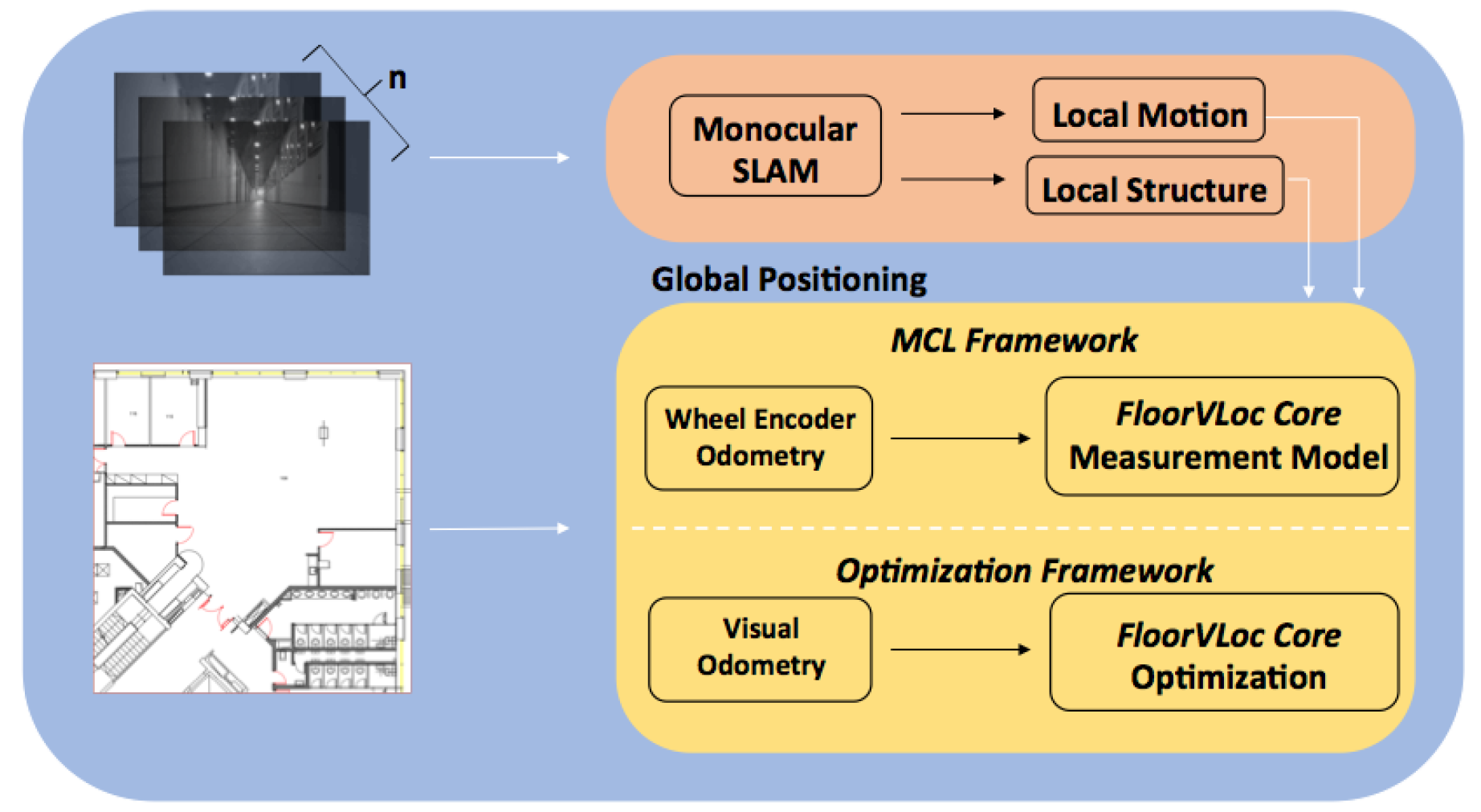
• Two full global positioning systems based on this methodology which perform continuous positioning at real-time computation rates. One approach utilizes visual odometry in between Floorplan Vision Vehicle Localization (FloorVLoc) linear optimization localization updates; another approach formulates the system in a Monte Carlo Localization (MCL) framework with a FloorVLoc measurement model, correcting motion based on whatever wall information is present shown in Figure 2.
• Experimental evaluation of the global positioning systems for indoor search and rescue applications in a challenging real-world environment, as well as real and simulation testing for a focused study of various aspects of the methodology.

2. Literature Review

One rather immediate indoor alternative to GPS/GNSS would be based on radio frequency, such as Wifi, Bluetooth, or Ultra-wideband (UWB), yet the requirement of new infrastructure installation or deployable equipment prevents it from being a feasible solution in the context of the present study [4,5,6,7]. Futhermore, due to the challenges associated with constructing and maintaining the map and the accuracy issues associated thereof, there has been an effort to integrate other sensors with radio frequency signals [8].

Image-Based Localization (IBL) [9,10,11,12] has broadly been a popular approach to localization due to the amount of information that is provided by images. State-of-the-art algorithms for IBL have continued to follow a 3D structure-based approach [13,14,15,16,17,18,19,20], where 2D-3D image point to 3D world point correspondences are established for a query image, and then the camera pose is solved using an n-point-pose (PnP) solver. Understandably, due to outliers in the data associations, the whole algorithm is often placed inside a robust framework (e.g., RANSAC [21]). Alternatively, Deep Convolutional Neural Networks have also been deployed in order to achieve Absolute Pose Regression (APR) where, rather than relying on machine learning for extracting local features or handling outliers, the camera pose is regressed directly from the network [22,23,24,25,26,27,28]. However, 3D structure-based approaches have continued to significantly outperform the APR ones since APR approaches cannot guarantee to generalize from the training data, and it has been shown that such approaches cannot outperform an image retrieval algorithm [29]. Furthermore, there are some issues of brittleness as updating the map requires retraining the CNN network. Therefore, there is quite a bit of room for further research in this area.

Similar IBL approaches have been used for indoors as well [18,30,31]. For example, fiducial markers have been utilized in an indoor localization framework; by specifying the 3D locations of such markers with respect to the indoor environment, the transformation between the marker and the camera can be obtained when recognizing it in the image [32,33,34]. Scale is resolved through specifying the size of the marker, and the orientation is computed based on the unique orientation of the marker pattern with respect to the camera. Another type of map that has been used is a multi-channel raster image of the building [35], where in addition to lines of the intersections between walls and the floor (like a floorplan), information about the current status of the environment is inserted, such as the contours of static objects and an occupancy grid map specifying information of available areas for the robot to navigate. In a similar fashion, another approach has been to create a distance function based map offline thereby providing information about both region occupancy and distances to the occupied areas [36]. One of the main drawbacks to approaching localization in such a way is the requirement to either install infrastructure in the environment or explore it before performing the localization. In fact, constructing and extending a large-scale 3D model of the world prior to online positioning often requires using a sensor of the same modality. Torii et al. investigated whether such models are required in contrast to 2D image retrieval-based methods relying on a database of geo-tagged images. Their experimentation shows that 3D large-scale models are not strictly required, and approaches which can combine image-based methods with local reconstructions produce accurate positioning solutions [37]. The focus on utilizing local reconstructions is the approach that is taken in this paper, but rather rather than relying on any type of large-scale 3D model, using a floorplan significantly alleviates the issue of map construction and maintenance, and further, it does not require environments to be explored beforehand. The approach in this paper utilizes local reconstructions and relates them to global planar information from the floorplan in order to achieve global positioning. While a monocular camera could be coupled with another type of map (e.g., a 3D point cloud lidar map) for localization by computing the similarity transformation between the local reconstruction and the global map [38], there are several advantages in choosing a floorplan to perform the indoor localization with this paper: First, from an application-context perspective, our method does not require the scene to be previously explored; second, using a floorplan provides more flexiblity for data association which is more critical in indoor settings where texture and features are not as prevalent as in outdoor settings; third, our method uses the minimal amount of prior map information required for global localization, an extra challenge which this paper solves.

While surprisingly somewhat rare, floorplans have been used as maps with localization systems before, and when they are used, they are primarily coupled with sensors which provide depth information (lidar or RGBD cameras). With regard to approaches using RGBD cameras, Ito et al. [39] approached localization in a Bayesian state estimation framework using a particle filter (i.e., Monte Carlo Localization) with an RGBD camera and IMU for visual-inertial odometry with the depth information provided by the depth camera utilized in the measurement process using a beam sensor model. Wifi signals were also integrated in order to help reduce multi-modality of the particle filter and increase the convergence speed. Winterhalter et al. [40] similarly utilized an RGBD camera and IMU to guide the proposal distribution, using the Google Tango Tablet platform where the depth data formed the basis of the measurement model, and localization operated in an MCL framework. Ma et al. [41] developed an RGBD Simultaneous Localization and Mapping (SLAM) system which combines direct image alignment frame-to-keyframe with frame-to-plane alignment via a global graph optimization. Coupling the local motion estimation with the global in the same optimization has the drawback of not being modular to using any underlying visual SLAM algorithm. Chu et al. [42] approached performing global localization using a monocular camera via full point cloud, line, and conservative free space matching by using a scaled-version of the reconstruction (therefore similar output to what one would get with an RGBD camera) from a semi-dense visual odometry algorithm. Computing the scale offline and then using it for matching means that such an approach cannot be performed online as it avoids automatic scale calibration, a critical issue which is solved in this paper. Mendez et al. [43,44] approached the problem from a different perspective where semantic information is extracted from the images and then matched to the floorplan to localize using the angular distribution of the semantic labels. Similarly, Wang et al. focused on utilizing text from the names of stores and facade segmentation in order to localize within a shopping mall [45]. With their approach, the text of store names was determined via a Markov Random Field (MRF) and accuracy was limited to around 1–5 m. Further, in situations when text was missing, the system suffered severely. Depth information of the scene has also been acquired via lidar which can be integrated into a pose-graph optimization rather than a filtering scheme. The data acquired by the lidar sensor can be utilized for odometry via scan-matching, and then an ICP algorithm can be deployed in order to use the floorplan and provide an a priori estimate on the pose, which is subsequently optimized according to the underlying pose graph [46,47].

Monocular SLAM/Visual Odometry (VO) has been researched somewhat extensively, including approaches such as ORB-SLAM2 [48], SOFT-SLAM [49], LDSO [50], NID-SLAM [51], ROCC [52], Fast-SeqSLAM [53], SVO [54], and PL-SVO [55]. Furthermore, the Bundle Adjustment algorithm has consistently been a state-of-the-art approach for jointly inferring 3D structure, typically sparse scene structure, and camera pose information from a series of images by minimizing the geometric reprojection error, and many SLAM formulations have relied on it [56,57,58,59,60]. In light of this, due to the known scale ambiguity issue, there has been a considerable amount of work to utilize monocular cameras to acquire metric depth information either from Deep Convolutional Neural Networks [61,62,63,64,65] or by relating visual cues to structural information in the scene for which metric scale can be known. One approach is to take advantage of the objects present in the scene, known as Object-SLAM. The goal is to recognize objects in the environment and compute the scale by utilizing priors on the sizes of such objects [66,67,68,69,70]. In general, such a problem deals with both robust object detection and object measurement [71,72,73]. Other geometric structures (e.g., the ground plane) have also been exploited to help resolve the scale [74,75,76,77,78]. Lastly, the visual information has also been often integrated with other sensors such as an IMU [79,80,81,82] or lidar [83,84,85].

In order to continuously provide global positioning so that local reconstructions can be properly matched to the global structure, perceptual information should be integrated into a system which fuses multiple sources of information effectively. Traditionally, Extended Kalman Filter approaches were utilized [86,87,88,89,90,91] for localization, but more recently, approaches based on particle filters especially for mobile robotics localization have been deployed [92,93,94,95,96], also known as Monte Carlo Localization (MCL). More rarely, however, has Bundle Adjustment been utilized to integrate various sources of external scene information with visual information into a formulation which can solve global positioning. One way is to augment the cost function to include these external constraints, and thereby perform a constrained Bundle Adjustment (BA) optimization [97,98,99]. Finally, one of the well-known challenges to overcome with vision-based navigation is drift. In contrast to sensors which can measure depth, monocular vision systems add another degree of freedom to drift over time with respect to scale. Thus, drift correction becomes of vital importance, and is addressed in a variety of ways [100,101,102]. For example, in [103], per-frame global optimizations are performed over all current and past camera poses while in other works techniques of loop closure or derivatives thereof have been required to resolve it (e.g., [104]). This paper addresses the drift issue by deriving the relationship between the vision-based data and the floorplan and explicitly providing mathematical criteria for showing when global localization computations can be drift-free based on the geometrical structure in view. While a floorplan typically offers more information, utilizing simply the planar information is sufficient to localize effectively and accurately.

3. Global Localization: The FloorVLoc Core

To give an overview of the global localization: a series of images taken by a moving monocular camera is processed by an underlying monocular SLAM algorithm which outputs local motion and scene structure. This paper provides two methods for performing this global positioning—one in a Monte Carlo Localization framework and the other via an optimization framework. The MCL framework combines the camera egomotion with wheel encoders to form a motion model and relies on a FloorVLoc Core measurement model to refine the localization. The optimization framework incorporates the local camera motion with a floorplan-based scale estimate to provide visual odometry and solves for the refined poses via a FloorVLoc Core optimization.

This section presents the core methodology for integrating a monocular camera with a floorplan to provide global localization. An emphasis is placed on the automatic scale calibration in an online fashion—a feature which is necessary in order to be able to use any underlying monocular SLAM system for online global positioning. In addition, an analysis is presented of the visual features associated with the walls to ensure unique global localization, which intrinsically corrects drift. The beauty of all of this comes from the fact that it can be derived from first principles and consequently has significant ramifications.

Suppose that the platform is moving and an image is taken at time t by the camera located at position $p\in {\mathbb{R}}^3$ with orientation denoted by $\mathbf{R}\in \mathrm{SO}\left(3\right)$. Further, suppose features are extracted from the image such that the i-th feature point has normalized homogeneous image coordinates of ${\overline{q}}_i\in {\mathbb{R}}^3$. Then the true location $Q_i$ of the corresponding feature is

$$Q_i=p+{\lambda }_i\mathbf{R}{\overline{q}}_i$$

(1)

where ${\lambda }_i$ is referred to as the depth of the ith feature point. Consider the estimated position $\widehat{p}$ and orientation $\widehat{\mathbf{R}}$ by the localization algorithm at the same time instant. Then the 3D location ${\widehat{Q}}_i$ can be expressed as:

$${\widehat{Q}}_i=\widehat{p}+{\widehat{\lambda }}_i\widehat{\mathbf{R}}{\overline{q}}_i$$

(2)

Assuming that ${\overline{q}}_i$ is a feature on the jth wall of the floorplan, then both ${\widehat{Q}}_i$ and $Q_i$ are 3D points which should lie on that wall. Let ${\pi }_j=(N_j,b_j)$ denote the planar properties of such a wall where $N_j$ is the normal vector and $b_j$ is the distance from the plane to the world origin. While the true location $Q_i$ is unknown, ${\widehat{Q}}_i$ can be estimated, and consequently the depth ${\widehat{\lambda }}_i$, by using a ray-tracing algorithm. Under this assumption, it directly follows that:

$$N_j^{\top }({\widehat{Q}}_i-Q_i)=0$$

(3)

Applying this to (2) and left-multiplying by $N_j^{\top }$, yields

$${\widehat{\lambda }}_i{N}_j^{\top }\widehat{\mathbf{R}}{\overline{q}}_i=N_j^{\top }(Q_i-\widehat{p})$$

(4)

Since $b_j=N_j^{\top }{Q}_i$ is the distance from the origin of the world coordinate system to the jth wall, (4) can be simplified to

$${\widehat{\lambda }}_i{N}_j^{\top }\widehat{\mathbf{R}}{q}_i=b_j-N_j^{\top }\widehat{p}$$

(5)

Consider next a sequence of images captured using the monocular camera and then processed using a monocular vision Simultaneous Localization and Mapping (SLAM) algorithm where the local motion and scene structure are recovered. Because depth computation is up to an unknown scalar s which is common to all of the points, ${\overline{\lambda }}_i=\frac{1}{s}{\widehat{\lambda }}_i$ Thus:

$$s{\overline{\lambda }}_i{N}_j^{\top }\widehat{\mathbf{R}}{\overline{q}}_i=b_j-N_j^{\top }\widehat{p}$$

(6)

Equation (6) can be used in either an optimization framework or integrated as a measurement process in a filtering framework. Both approaches will be presented with a study of certain planar criteria which must be met to uniquely compute the pose.

3.1. Optimization Framework (FloorVLoc-OPT)

Suppose that $\widehat{\mathbf{R}}$ is a good approximation to the true orientation $\mathbf{R}$ so that

$$\mathbf{R}=\Delta \Psi \widehat{\mathbf{R}}$$

(7)

where $\Delta \Psi$ is a small rotation matrix (approximately equal to the identity matrix $\mathbf{I}$). Using the small angle approximation and the wedge operator ${(·)}^{\wedge }$, which converts 3D vectors into 3 × 3 skew-symmetric matrices,

$$\Delta \Psi \approx \mathbf{I}+\Delta {\psi }^{\wedge }$$

(8)

with

$$\Delta \psi =\left(\begin{array}{c}\delta \varphi \\ \delta \theta \\ \delta \psi \end{array}\right)$$

(9)

$\delta \varphi$, $\delta \theta$, and $\delta \psi$ being small angles. Using this approximation, (6) can be rewritten as

$${\overline{\lambda }}_i{N}_j^{\top }(\mathbf{I}+\Delta {\psi }^{\wedge })\widehat{\mathbf{R}}{\overline{q}}_i=\frac{1}{s}(b_j-N_j^{\top }p)$$

(10)

The estimate for the pose is obtained by scaling the camera egomotion from the underlying monocular SLAM algorithm and transforming it based on a world reference pose. The world reference pose is chosen to be the last one for which a global localization solution was computed or the initial world pose. Defining $\overline{p}=\frac{1}{s}\widehat{p}$ and after some algebra, (10) becomes

$${\overline{\lambda }}_i{N}_j^{\top }{\left(\widehat{\mathbf{R}}{\overline{q}}_i\right)}^{\wedge }\Delta \psi +\frac{1}{s}{b}_j-N_j^{\top }\overline{p}={\overline{\lambda }}_i{N}_j^{\top }\widehat{\mathbf{R}}{\overline{q}}_i$$

(11)

which in matrix form looks like:

$$\left[\begin{array}{ccc}{\overline{\lambda }}_i{N}_j^{\top }{\left(\widehat{\mathbf{R}}{\overline{q}}_i\right)}^{\wedge }& b_j& -N_j^{\top }\end{array}\right]\left[\begin{array}{c}\Delta \psi \\ \frac{1}{s}\\ \overline{p}\end{array}\right]={\overline{\lambda }}_i{N}_j^{\top }\widehat{\mathbf{R}}{\overline{q}}_i$$

(12)

Note that (12) provides one constraint on the variables of the problem. Assuming that a sufficiently large number of such equations are collected so that the associated matrices have full rank (more on this later), the resulting linear system of equations can be solved efficiently. If required, the small angle approximation can be relaxed by replacing $\widehat{\mathbf{R}}\leftarrow \Delta \Psi \widehat{\mathbf{R}}$ after finding the angular perturbation and performing a new iteration of the above algorithm to refine the solution. Here $\Delta \Psi$ should be formed as the rotation matrix associated with $\Delta \psi$ and not its small-angle approximation.

3.2. Planar Motion

The constraints developed in the previous section can be used as the basis for global localization for six degree of freedom platforms (e.g., quadcopters, mobile phones). However, because the platform of interest for search and rescue is a small robotic vehicle, in this section we will elaborate on the specialization to planar motion. Suppose then that a ground vehicle is used to carry the camera which is furthermore assumed to be rigidly mounted. Using the assumption that changes in height and roll and pitch angles are negligible, the orientation perturbation reduces to $\Delta \psi ={(0,0,\delta \psi )}^{\top }$ and by defining $c_{\psi }=cos\left(\psi \right)$ and $s_{\psi }=sin\left(\psi \right)$ so that

$$\begin{array}{cc}\hfill & {\alpha }_{ij}={\overline{\lambda }}_i{N}_{j_x}(s_{\psi }{q}_{i_x}+c_{\psi }{q}_{i_y})+N_{j_y}(s_{\psi }{q}_{i_y}-c_{\psi }{q}_{i_x})\hfill \\ \hfill & {\gamma }_{ij}={\overline{\lambda }}_i{N}_{j_x}(c_{\psi }{q}_{i_x}-s_{\psi }{q}_{i_y})+N_{j_y}(s_{\psi }{q}_{i_x}+c_{\psi }{q}_{i_y})+N_{j_z}{q}_{i_z}\hfill \end{array}$$

(13)

where ${(·)}_x,{(·)}_y,$ and ${(·)}_z$ denote the x, y, and z components of the vector, respectively, (11) becomes:

$${\alpha }_{ij}·\delta \psi +\frac{1}{s}{b}_j-N_j^{\top }\overline{p}={\gamma }_{ij}$$

(14)

Again, in matrix form:

$$\left[\begin{array}{cccc}{\alpha }_{ij}& b_j& -N_{j_x}& -N_{j_y}\end{array}\right]\left[\begin{array}{c}\delta \psi \\ \frac{1}{s}\\ {\overline{p}}_x\\ {\overline{p}}_y\end{array}\right]={\gamma }_{ij}$$

(15)

3.2.1. Data Association

One of the key components to effectively perform the global positioning is the data association. Planar associations are found between the map points from the underlying SLAM algorithm across some designated time horizon and the global planes ${\pi }_j$ provided by the building floorplan. The associations are found by performing ray tracing. During the initial stage of the algorithm, before any scale factor has been computed, all planar associations are kept; however, in subsequent stages, once a scale factor has been computed, then associations undergo an outlier filtering process. The planar fitting error ${ϵ}_i^j$ derived from (6) is computed for every point-plane association $(q_i,{\pi }_j)$:

$${ϵ}_i^j=b_j-N_j^{\top }(s\mathbf{R}{\overline{q}}_i+\widehat{p})$$

(16)

Note that $q_i$ are all the points across some time horizon (meaning points from the past are propagated to the current pose coordinate frame). Associations are only kept when $|{ϵ}_i^j|<\tau$ where $\tau$ is some threshold. For the experimentation in this paper, $\tau$ was chosen to be 30 cm. Because some points have more error than others either due to triangulation error or due to obstacles in the environment, the planar fitting error can be used to formulate a weight for each planar association and a weighted least squares optimization can be performed using (15). The weights are defined to be:

$$w_i^j=exp\left(-\frac{({ϵ}_i^j-{\mu }_j)}{2{\sigma }_j^2}\right)$$

(17)

where ${\mu }_j$ and ${\sigma }_j$ are the mean and standard deviation, respectively, of the planar fitting error for all points on plane j. If there are fewer than 10 associated points to some plane, those points are discarded to mitigate outliers. In addition, due to the fact that a robotic vehicle has planar motion, only vertical planes constrain the localization, and thus only points on vertical planes are utilized for the optimization. Lastly, in order to be more robust to incorrect solutions, pose computations are only accepted if their corresponding positions and orientations are a weighted threshold away from the a priori estimated poses, with weight proportional to the time since the last computed localization solution.

3.2.2. Initialization

The vehicle starts from a known world pose but an estimate for the scale needs to be computed. This is done by finding planar associations as described in Section 3.2.1 and obtaining a scale factor for each association $(q_i,{\pi }_j)$ by:

$${\widehat{s}}_i=\frac{b_j-N_j^{\top }p}{N_j^{\top }\mathbf{R}{q}_i}$$

(18)

The overall estimate is computed by taking the median of all scale factors:

$$\widehat{s}=\mathrm{med}{\widehat{s}}_i$$

(19)

Using the median is advantageous for handling potential outliers. In addition, here we consider points on all planes including horizontal planes such as the ground or ceiling. While such points do not affect the position or orientation for the vehicle, they can be used to compute the scale which is necessary for initializing the system using the floorplan. So in this context, such points are useful to include. This scale factor is then refined when the linear optimization is performed.

3.2.3. Uniqueness Criteria

In order to uniquely compute the pose of the camera using the planar associations, certain planar criteria must be met which are manifested in the rank of matrix (12) for the general case and matrix (15) for a vehicle. For the general case, (12) is a linear system of equations with seven unknowns, and hence at least seven distinct visual features must used. To determine the requirements for computing a unique camera pose based on planar criteria, let ${\mathbf{A}}_{\pi }$ be the matrix of the k world planes that are in view across the time horizon and be defined as follows:

$${\mathbf{A}}_{\pi }=\left[\begin{array}{cc}{b}_1& -N_1^{\top }\\ b_2& -N_2^{\top }\\ ⋮& \\ b_k& -N_k^{\top }\end{array}\right]$$

(20)

Then the following result holds:

Lemma 1.

A necessary and sufficient condition for computing a unique pose is that seven distinct feature points are visible and the matrix $A_{\pi }$ has rank at least four.

Proof. 

See Appendix A. ☐

In considering the uniqueness criterion for a robotic vehicle platform where planar motion occurs, define the matrix ${\mathbf{A}}_{\pi }^v$ to be:

$${\mathbf{A}}_{\pi }^v=\left[\begin{array}{ccc}{b}_1& -N_{1_x}& -N_{1_y}\\ b_2& -N_{2_x}& -N_{2_y}\\ ⋮\\ b_k& -N_{k_x}& -N_{k_y}\end{array}\right]$$

(21)

In this special case, the conditions in Lemma 1 can be reduced:

Lemma 2.

A necessary and sufficient condition for computing a unique pose for a camera rigidly mounted onto a robotic vehicle is that four distinct feature points are visible and the matrix ${\mathbf{A}}_{\pi }^v$ has a rank of at least three.

Proof. 

See Appendix B. ☐

3.3. Monte Carlo Localization Framework (FloorVLoc-MCL)

The second approach presented in this paper for monocular floorplan localization which can utilize any underlying monocular SLAM algorithm is based on a Monte Carlo Localization (MCL) [105] framework. MCL is achieved via the Bayesian recursive update, where each particle ${\mathbf{x}}_t$ represents a pose hypothesis and

$$bel\left({\mathbf{x}}_t\right)\propto p\left({\mathbf{z}}_t\right|{\mathbf{x}}_t){\int }_{X}p\left({\mathbf{x}}_t\right|{\mathbf{x}}_{t-1},{\mathbf{u}}_t)\mathit{bel}\left({\mathbf{x}}_{t-1}\right)d{\mathbf{x}}_{t-1}$$

(22)

where ${\mathbf{z}}_t$ denotes the measurement and ${\mathbf{u}}_t$ refers to the control, which in this context corresponds to odometry. The particles are propagated according to a motion model $p\left({\mathbf{x}}_t\right|{\mathbf{x}}_{t-1},{\mathbf{u}}_t)$ and then re-weighted based on a measurement model $p\left({\mathbf{z}}_t\right|{\mathbf{x}}_t)$ in order to estimate the posterior belief of pose ${\mathbf{x}}_t$. The particles are initialized uniformly using the a priori pose estimate and its uncertainty, and the scale component of each particle is initialized using the method given in Section 3.2.2.

3.3.1. Motion Model

More specifically, because the particles are elements of the Lie Algebra $\mathfrak{sim}\left(2\right)$ (position, orientation, and scale), the scale of the scene must also be taken into account in the motion model so that each particle can properly and effectively propagate the scale forward. The position and orientation use a standard odometry motion model with Gaussian error terms in a three-vector parameterized form. The odometry is obtained using the wheel encoders for distance and the camera egomotion from the underlying SLAM algorithm for relative orientation. Let ${\mathbf{x}}_t$ denote the estimated current pose updated from the odometry motion model, ${\mathbf{x}}_{t-1}$ refer to the pose at the previous time step, and the corresponding poses from the camera egomotion be ${\xi }_{t-1},{\xi }_t$. The estimated scale for each particle is computed by

$$s_t=\frac{\left|\right|{\mathbf{x}}_t^{\mathrm{tr}}-{\mathbf{x}}_{t-1}^{\mathrm{tr}}\left|\right|}{\left|\right|{\xi }_t^{\mathrm{tr}}-{\xi }_{t-1}^{\mathrm{tr}}\left|\right|}$$

(23)

where ${(·)}^{\mathrm{tr}}$ refers to the translation component of the pose vector. This way, the scale can be propagated in a way that is coupled to the propagation of the position of each particle.

3.3.2. Measurement Model

The measurement model of MCL is used to integrate the global planar information provided by the floorplan and the reconstructed local scene structure in order to re-weight the propagated pose hypotheses. The general idea is to compute the planar fitting error for all of the points, placing them on their respective walls, according to each specific pose hypothesis. This formulates the log-likelihood of the measurement. In order to accomplish this, associations are established according to the method described in Section 3.2.1 except no outlier filtering is performed here. The measurement log-likelihood is then defined as,

$$logp\left({\mathbf{z}}_t\right|{\mathbf{x}}_t)=-\frac{1}{2m{\sigma }_z^2}\sum _{i=1}^m\rho \left(b_j-N_j^{\top }(s\mathbf{R}{q}_i+p)\right)$$

(24)

where $\mathbf{R}$ is the rotation matrix corresponding to the orientation component of ${\mathbf{x}}_t$, p is the translation component of ${\mathbf{x}}_t$, and s is the scale component of ${\mathbf{x}}_t$. Furthermore, $\rho (·)$ is a robust kernel (e.g., Huber) to help mitigate outliers and ${\sigma }_z$ is a saturation term. In the experimentation presented in this paper, the odometry between the previous and current poses, $d_{t_1\to t_2}$, along with a constant $\kappa$ were used to define ${\sigma }_z$ as:

$${\sigma }_z=\frac{\kappa }{1+d_{t_1\to t_2}}$$

(25)

which effectively places less weight on measurements with small baselines. The justification for this is that the accuracy of Bundle Adjustment (from Multi-View Geometry) increases with longer baselines. The tuning parameter $\kappa$ was chosen to be 100 for the experimentation presented later in the paper.

Each particle is then updated by the following weight policy, which experimentally was verified to work well:

$$w=\frac{1}{1-logp\left({\mathbf{z}}_t\right|{\mathbf{x}}_t)}$$

(26)

After re-weighting the particles, then all of the particles are re-sampled using stochastic universal resampling, and the process repeats recursively according to (22).

4. Experimental Evaluation

In order to evaluate the performance of our proposed approach, we collected data using a robotic vehicle equipped with the uEye IDS monocular camera (IDS Imaging Development Systems GmbH); the camera was forward facing and mounted at a height of about 15 cm off the ground. The external odometry was based on wheel encoders, and the vehicle sensor array also included an Odroid XU4 (Ameridroid High-Performance Electronics) onboard computer and an Arduino Nano. The odometry from the wheel encoders was somewhat poor, yielding an error of about 5%. The on-board camera provided up to 57 fps at full resolution of 3.2 MP with a field of view of 65.6 × 51.6 degrees. The length of the vehicle was 53.5 cm and its width was 28.1 cm—which is important to note in light of the accuracy of the systems. For the tests presented, the vehicle was used for data acquisition, and the positioning systems were run offline on a laptop computer. Two types of image resolutions were experimented with when running the local monocular SLAM system [48] which was used for all of the experimentation: The optimization framework used $2056\times 1542$, and the MCL framework used $640\times 480$. For both systems, the initial ground-truth pose in the floorplan was given. Note that the floorplan, which was obtained from building managers, contained the ceiling height. Details on how ground truth was obtained are given in Appendix C.

4.1. Comparison to Related Methods

The positioning algorithms presented in this paper, FloorVLoc-OPT and FloorVLoc-MCL, which correspond to the optimization and MCL frameworks, respectively, were compared to each other as well as to a state-of-the-art SLAM algorithm, ORB-SLAM. Because ORB-SLAM is a monocular SLAM algorithm, the map built is with respect to the initial camera pose and the trajectory is without scale. We align ORB-SLAM’s initial pose with the ground truth initial world pose and scale the trajectory via two different ways: The first way computes the ratio of the distance between two known ground-truth positions and the corresponding unscaled distance between two ORB-SLAM positions.

$$s_1=\frac{\left|\right|{\left({\mathbf{x}}_{t_2}^{GT}\right)}^{\mathrm{tr}}-{\left({\mathbf{x}}_{t_1}^{GT}\right)}^{\mathrm{tr}}\left|\right|}{\left|\right|{\left({\xi }_{t_2}\right)}^{\mathrm{tr}}-{\left({\xi }_{t_1}\right)}^{\mathrm{tr}}\left|\right|}$$

(27)

The second way uses the distance obtained from the external odometry provided by the wheel encoders rather than the translation between two ground truth poses.

$$s_2=\frac{d_{t_1\to t_2}}{\left|\right|{\left({\xi }_{t_2}\right)}^{\mathrm{tr}}-{\left({\xi }_{t_1}\right)}^{\mathrm{tr}}\left|\right|}$$

(28)

where $d_{t_1\to t_2}$ is the wheel encoder odometry between two selected poses used for the scale computation. Note that the latter can be implemented in real-time while the former is useful for experimentation.

The results for the FloorVLoc-MCL and FloorVLoc-OPT global positioning systems as well as the comparison approaches are given in

Table 1. Results for the FloorVLoc global positioning systems across a trajectory of about 8000 cm. The errors are found by taking the error vector between each pose and its corresponding ground truth and computing the mean error vector ($\overline{\mathbf{e}}$) and the covariance matrix from which the standard deviation $\overline{\sigma }$ is obtained.

Method	${\overline{\mathit{e}}}_{\mathit{pos}}$ (cm)	${\overline{\mathit{\sigma }}}_{\mathit{pos}}$ (cm)	${\overline{\mathit{e}}}_{\mathit{ori}}$ (rad)	${\overline{\mathit{\sigma }}}_{\mathit{ori}}$ (rad)
ORB-SLAM with Odometry Scale	(151.31, 43.66)	(202.65, 34.58)	0.0088	0.019
ORB-SLAM with GT Scale	(23.67, 37.46)	(249.59, 42.24)	0.0088	0.019
FloorVLoc-OPT	(5.86, 8.00)	(10.90, 19.34)	0.00035	0.046
FloorVLoc-MCL	(5.92, 3.37)	(40.10, 7.86)	0.00066	0.080

.

Trajectories for both FloorVLoc algorithms are shown in Figure 3a,b. The vehicle started in a more open area and then proceeded down a long corridor, making a loop around an island of offices containing rather narrow corridors and very tight turns, and then returning to the open area. During the execution, there were dynamic obstacles (e.g., people walking in front of the vehicle at multiple instances, sometimes right in front) as well as static obstacles (e.g., cabinets) and other challenging aspects such as significant illuminance variation due to sunlight entering windows. Handling dynamic obstacles is usually a front-end task and one which has been directly tackled in the literature [106,107], and its negative result is typically manifested in tracking difficulty or reconstructed points which need to be treated as outliers for floorplan-based localization. Due to the modular design of the global positioning systems in this paper, the focus on dealing with dynamic obstacles was placed on properly handling outliers in the reconstructed scene as discussed in Section 3.2.1.

First of all, it can be seen that the FloorVLoc algorithms significantly outperformed the ORB-SLAM transformed trajectories. Whereas both ORB-SLAM ones expectedly suffered from drift significantly, the FloorVLoc approaches properly handled the drift as shown in Figure 4, which was one of the main benefits of incorporating the floorplan into the global positioning. It can also be seen that the main sources of error were in the X direction, which is related to the fact that this was the direction of the corridor, and consequently, the majority of the motion was in the X direction. Furthermore, it can also be seen that the motion in the Y direction was properly constrained as the error was quite small and relatively consistent throughout despite the trajectory containing a loop around the island of offices. Even though there were people that walked around the moving vehicle at three separate instances throughout the execution, it can be seen that the error was still low, with standard deviation even less than the length of the vehicle itself.

One of the interesting places in the experimentation happened around frame 1534 where in Figure 5 we can see the uncertainty of the underlying monocular SLAM algorithm The vehicle was in the process of turning out of the island of offices and encountered a situation where there was primarily a white wall and the floor—a classic place for tracking failure—and indeed tracking often did at this point. Figure 5 also shows a rise in the uncertainty in the Bundle Adjustment optimization during that time period. Figure 5 is a plot of the pose inverse Hessian norm of the local Bundle Adjustment optimization the last time that a particular frame was part of the optimization. Understandably, the uncertainty could not be directly related to global pose uncertainty because of the correlations which existed between camera poses and due to the fact that the uncertainty for the poses in the local BA were with respect to the keyframes, which were fixed to handle the gauge freedom. Nevertheless, it was indicative of places in the trajectory when the underlying local SLAM had more difficulty. In fact, errors in the local reconstruction from the windowed BA optimization will propagate to the global positioning system similar to how sensor errors propagate into the error of any localization system. This is inherent to the design of the system which was done in order to keep modularity so that any underlying SLAM algorithm could be used and computational cost could be kept at a minimum. The important point to note is that while SLAM systems have to deal with long-term drift, the FloorVLoc methods provide the means to correct drift and localize with respect to the building.

Therefore, it can be seen that the orientation error shown in Figure 6, particularly for FloorVLoc-MCL, increased during that time; however, the error subsequently decreased utilizing the walls of the floorplan to guide its correction. For that area, the orientation error for FloorVLoc-OPT increased but not as much. Note that the OPT approach uses a larger horizon when computing the pose, whereas the MCL approach used the current points that the camera views for updating the motion in the measurement model. One of the benefits of using a larger horizon is that challenging tracking situations can be handled more effectively, as can be seen by the results. However, it should be noted that as the horizon increased, the influence of drift naturally also increased since technically drift was only eliminated when only the points in the current BA optimization were used. FloorVLoc-OPT used a horizon of 15 keyframes which provided a nice balance. Overall, while both FloorVLoc approaches performed very well for the challenging dataset, the optimization-based approach tended to outperform the MCL approach.

For the MCL approach, the initial pose was assumed to be known with an uncertainty modeled by zero-mean Gaussian noise with a standard deviation of 10 cm in the position and 10 degrees in the orientation. Ten runs of the algorithm were performed in order to incorporate the stochastic nature, and the results were averaged. Figure 4 and Figure 6 plot the averaged results for the position and orientation errors. In Figure 7, the average error as well as the standard deviation of the error across all runs are plotted.

4.2. Ablation Study

4.2.1. FloorVLoc-MCL

In this section, we perform an ablation study of the localization algorithms under more controlled simulation environments. In order to further test specifically the MCL approach, which is probabilistic in nature, we constructed an indoor building in simulation using Unreal Engine 4 and Microsoft Airsim. Refer to Figure 8 for a view of the indoor simulation environment. The environment was built to emulate specific characteristics of indoor buildings. Obstacles such as a cabinet and bookshelf were placed to serve as planar obstacles and other obstacles such as a sofa and a chair were added to provide exposure to non-planar obstacles. The simulation building also contained windows with sunlight glare, a door, a lamp hanging from the ceiling, and other features so that the environment provided a reasonably realistic scenario for additional testing. Odometry was simulated by taking the ground-truth positions, computing the distance between them and accumulating a 5% error on the distance, similar to what happens with the wheel encoders in the real data testing. The vehicle’s trajectory was designed so that the vast majority of the environment could be in view at some point. The camera parameters of the simulation camera were chosen to be similar to the ones with the real IDS camera. The camera was also placed at a similar height (15 cm). Ten runs of the algorithm were performed in order to incorporate the stochastic nature of the MCL framework and the positioning results were subsequently averaged. The initial pose was perturbed from the ground truth with a position error of 7.07 cm and an orientation error of 0.02 rad.

The trajectory along with the floorplan of the environment are shown in Figure 9. The average position error in the X and Y directions was 13.94 cm and 12.59 cm, respectively. The average standard deviation of the errors in the X and Y directions was 10.29 cm and 18.57 cm, respectively. The average orientation error was 0.086 rad and the standard deviation of the orientation error was 0.080 rad. The trajectory length was about 1570 cm. As the results demonstrate, there is consistency in the magnitude of error between the real data results and the simulation results, which is nice to observe.

4.2.2. FloorVLoc-OPT

In this section, we perform controlled experiments for single camera localization based on the planarity in the scene and study the effect of various sources of error including noise due to triangulation of points, data associations, and estimated prior camera pose.

The synthetic dataset used in this section, Tech-S-1, was generated with various environments and artificial floorplans (refer to Figure 10), according to a number of varying parameters. More specifically, all of the points were perturbed with some artificial pixel noise, ranging from ± half a pixel according to a uniform distribution. For the various synthetic tests, parameters varied across the initial orientation error, the number or percentage of incorrect correspondences, the number of planes in the scene (which sometimes included a planar obstacle such as a cabinet), the number of points per plane, the structure of the synthetic environment, the magnitude of the error resulting from the incorrect correspondences, artificial scale factor noise, and whether a robust estimation framework was set in place to handle the outliers. All of these details along with the localization results are summarized in

Table 2. Results of synthetic tests of FloorVLoc Core.

Parameters	Test 1	Test 2	Test 3	Test 4	Test 5	Test 6	Test 7	Test 8	Test 9
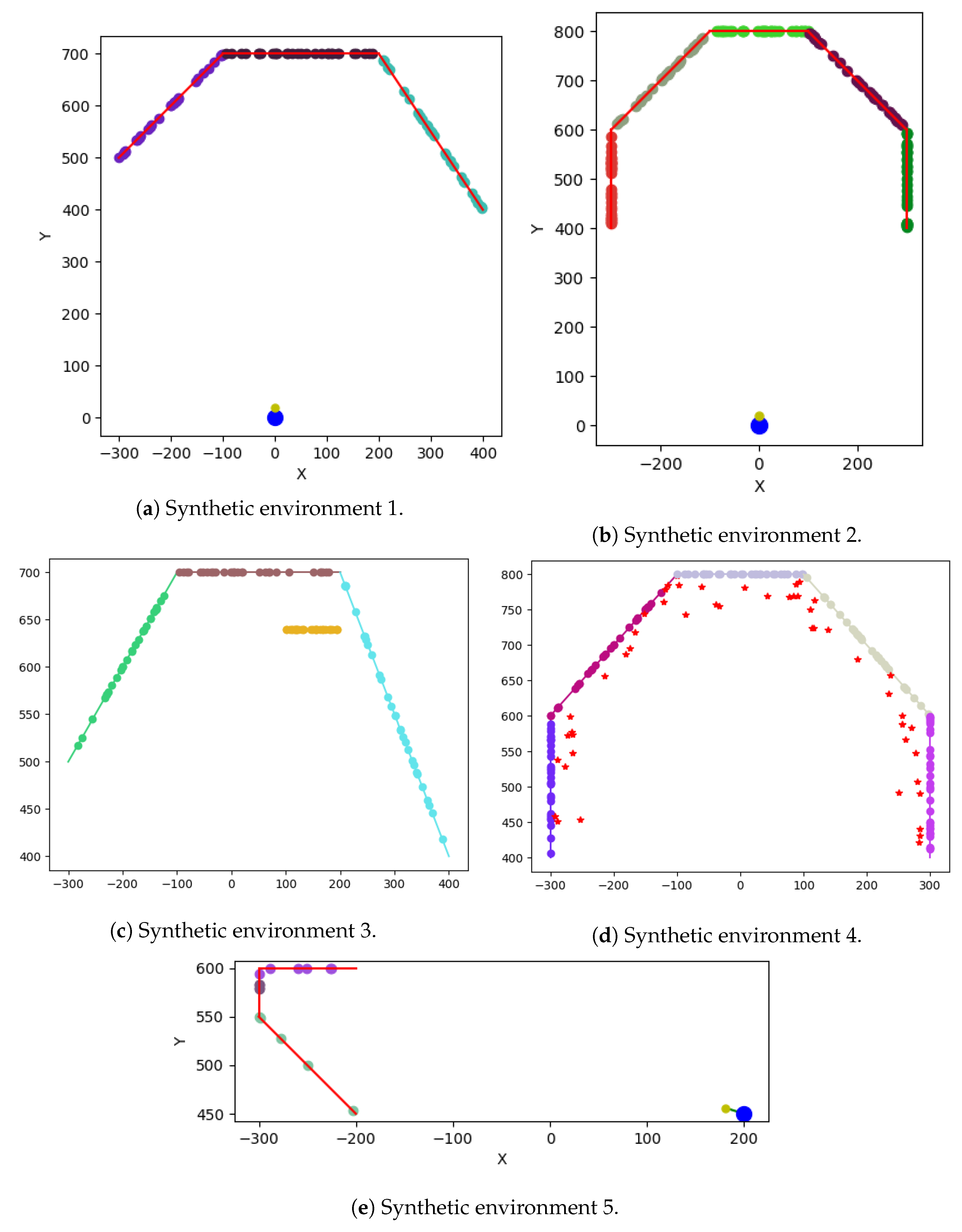
Synthetic Environment	1	1	1	5	2	2	4	1	3
Init Ori Error (rad)	0	0	0	0.04	0	0.02	0	0	0
Incorrect Correspondences	0	1	1	1	53.3%	53.3%	50	40%	30
Single Incorrect Corres. Error (cm)	-	3.6	193.2	-	-	-	-	-	-
Num Planes	3	3	3	3	5	5	5	3	4
Num Points/Plane	30	30	30	5	30	30	30	30	30
Robust Estimation	-	-	-	-	✓	✓	✓	✓	✓
Pixel Noise [–0.5, 0.5] px	✓	✓	✓	✓	✓	✓	✓	✓	✓
Scale Factor Noise	0	0	0	0	0	0	0	$1+\mathcal{N}(0,{0.1}^2)$	0
Position Error (cm)	(–0.05, –0.15)	(–0.19, 0.49)	(–23.2, 31.2)	(0.267, 6.36)	(0.88, 0.49)	(–0.49, 0.62)	(0.05, –0.07)	(0.32, 7.6)	(0.44, 0.16)
Orientation Error (rad)	0.0001	0.0006	0.074	0.01468	0.0016	0.001	0.0041	0.0002	0.0017

. Note that the position error refers to the magnitude of the position error vector, and the symbols “✓” and “-” correspond to a specific parameter being present or absent, respectively.

Test 1 serves as an initial benchmark to present the accuracy under somewhat ideal conditions. Here, the noise introduced into the system resulted only from the artificial pixel noise. In tests 2 and 3, a single data misassociation was made to investigate its effect on the localization. The results show the correlation between the position accuracy and the error of the misassociation projected along the plane’s normal. In test 2, the error resulting from the misassociation was relatively low (3.6 cm) and the position accuracy matched that, whereas in test 3, the error from the incorrect association was quite large (193.2 cm), and this caused the position accuracy to degrade somewhat. Test 4 examined what happened when the misassociation was on a wall which had a normal vector orthogonal to the wall it should be on. The results indicated that the orthogonal normal vector did not have a significant, negative effect on the positioning accuracy as long as the distance from the misassociated point to its correct wall was sufficiently close, which in this case was less than 10 cm. In tests 5–9, the localization algorithm from FloorVLoc Core was placed into a Random Sample Consensus (RANSAC) [21] framework in order to observe the effect of a significant increase in outliers. In test 5, 53.3% of the data had incorrect correspondences; in test 6, the same percentage of incorrect correspondences was coupled with initial orientation error; and in test 7, the outliers on the walls are shown in Figure 10d. Test 8 introduced perturbations in the scale for 40% of the data where the error was multiplicative Gaussian. More specifically, the depth for each point ${\lambda }_i$ was perturbed to be ${\tilde{\lambda }}_i=(1+{\delta }_{\lambda }){\lambda }_i$ where ${\delta }_{\lambda }\sim \mathcal{N}(0,{0.1}^2)$. Lastly, in test 9, a planar obstacle (simulating a cabinet for example) was introduced into the environment. Note that according to the localization criteria from Section 3.2.3 a positioning solution was still viable even with the planar obstacle, due to the geometrical properties of the walls, provided that the outliers from the planar obstacle could be handled (which they were in this test).

In addition to performing these localization tests using synthetic data, real data from our Tech-R-1 dataset were used to further investigate and understand the algorithms that could result from FloorVLoc Core. The reconstructed unscaled point cloud shown in Figure 11 and corresponding floorplan shown in Figure 12. The real data were collected by our robotic platform and subsequently processed by a monocular SLAM algorithm [48]. For the tests presented below, in order to handle the outliers which existed in the real data, the localization was performed inside an MSAC robust estimator [108] augmented with a regularization term. This was motivated by the fact that sometimes an obstacle in view contained a high number of features compared with the surrounding walls. In these cases, an estimation solution treating such obstacle points as belonging to nearby walls would have a comparatively lower cost due to the large support from the high number of features. The effect was that the position solution would be incorrect while the orientation solution could still potentially be correct. In order to handle this, a regularization term was incorporated utilizing a weighting parameter $\gamma$:

$$\mathcal{L}=(1-\gamma )\sum _i\rho {\left(e_i\right)}^2+\gamma \left|\right|\widehat{p}-\overline{p}{\left|\right|}^2$$

(29)

where $\overline{p}$ is the estimated a priori position. In the real testing above, $\gamma$ was chosen to be 0.5, and here $\rho (·)$ refers to the MSAC robust estimator kernel.

4.2.3. Test 1—Scale Perturbation

In this test, the scale factor was perturbed with Gaussian multiplicative noise while the initial orientation and position were unperturbed at their correct values. More specifically, $\tilde{s}=(1+{\delta }_s)s$ where ${\delta }_s\sim \mathcal{N}(0,{0.1}^2)$. The localization algorithm was run 30 times with different scale factors each time, and the position and orientation solution values were averaged across all of the runs before computing the error. For all of the tests in this section, the position error refers to the magnitude of the error vector. The average position error was 0.26 cm and the average orientation error was 0.013 rad.

4.2.4. Test 2—Initial Orientation Perturbation

For this test, the initial orientation was perturbed with Gaussian noise using a standard deviation of about 7 degrees while the initial position and scale were unperturbed at their correct values. In other words, ${\tilde{\psi }}_0\sim \mathcal{N}({\psi }_0,{0.1222}^2)$. Thirty iterations were run with different initial orientations each time. The average position error was 1.03 cm and the average orientation error was 0.030 rad.

4.2.5. Test 3—Initial Position Perturbation

In this test, the initial position was perturbed with Gaussian noise using a standard deviation of 30 cm in both the X and Y directions while the initial orientation and scale were unperturbed at their correct values.

Thus, ${\left[\begin{array}{cc}{\tilde{x}}_0& {\tilde{y}}_0\end{array}\right]}^{\top }\sim \mathcal{N}\left({\left[\begin{array}{cc}{x}_0& y_0\end{array}\right]}^{\top },{\left[\begin{array}{cc}{30}^2& {30}^2\end{array}\right]}^{\top }\right)$. Fifty iterations were run with different starting positions each time. The average position error was 7.90 cm and the average orientation error was 0.003 rad.

4.2.6. Test 4—All Perturbation

In this test, the initial position, initial orientation, and scale were all perturbed each run of the algorithm, and fifty runs of the algorithm were performed. The distribution of noise for each variable had the same parameters as specified in the three tests above. The average position error was 2.71 cm and the average orientation error was 0.027 rad.

4.3. Runtime

For all experimentation, a 6-core 2.8 GHz (with a 4.7 GHz turbo boost) Intel Xeon CPU was used. The average runtime for the MCL update was $(40\pm 15)$ ms (i.e., approximately 25 Hz) and the average runtime for the optimization framework update was $(0.14\pm 0.09)$ ms. In addition, the windowed Bundle Adjustment optimizations with the underlying SLAM system ran on average for $(129\pm 86)$ ms. This was measured for the $640\times 480$ image resolution. As mentioned above and shown in Figure 13, the additional processing time for providing global positioning was very low, especially with the optimization framework, which was 0.1% the computational time of the BA algorithm. This shows that these global positioning modules ran in real time to provide online global positioning.

5. Conclusions

In this work, we address vision-based indoor exploration by presenting a core methodology which combines a monocular camera with a floorplan to perform global positioning for a robotic vehicle. The main advantage of our approach is its modular nature: our method integrates any monocular-based local scene reconstruction with a floorplan to perform global localization, incorporating a means to automatically calibrate the scale. This means that any state-of-the-art monocular visual SLAM system can be directly utilized for the global positioning. A detailed theoretical and experimental analysis is presented for the conditions on the visual features associated with the walls necessary for the localization to be uniquely recovered. Furthermore, we developed two full global positioning systems based on the core methodology which perform continuous positioning. One approach utilizes visual odometry in between FloorVLoc linear optimization localization updates; another approach formulates the system in an MCL framework with a FloorVLoc measurement model, correcting motion based on whatever wall information is present. We demonstrate the effectiveness of FloorVLoc with experimental evaluation in the real world as well as in simulation, using Unreal Engine and Microsoft Airsim. Results for a challenging real-world dataset demonstrate robust, reliable, and accurate positioning with an average error of 0.06 m across a mission covering 80 m. Furthermore, we show that the FloorVLoc computational time is 0.1% the update time of the underlying monocular SLAM algorithm, thus operating in real-time. Based on these results, we conclude that FloorVLoc can be effectively deployed on an intelligent vehicle for the indoor search and rescue application of interest.

References

- Mouradian, C.; Yangui, S.; Glitho, R.H. Robots as-a-service in cloud computing: Search and rescue in large-scale disasters case study. In Proceedings of the 15th IEEE Annual Consumer Communications & Networking Conference (CCNC), Las Vegas, NV, USA, 12–15 January 2018; pp. 1–7. [Google Scholar]
- Whitman, J.; Zevallos, N.; Travers, M.; Choset, H. Snake robot urban search after the 2017 mexico city earthquake. In Proceedings of the 2018 IEEE International Symposium on Safety, Security, and Rescue Robotics (SSRR), Philadelphia, PA, USA, 6–8 August 2018; pp. 1–6. [Google Scholar]
- Martell, A.; Lauterbach, H.A.; Nuchtcer, A. Benchmarking structure from motion algorithms of urban environments with applications to reconnaissance in search and rescue scenarios. In Proceedings of the 2018 IEEE International Symposium on Safety, Security, and Rescue Robotics (SSRR), Philadelphia, PA, USA, 6–8 August 2018; pp. 1–7. [Google Scholar]
- Sun, W.; Xue, M.; Yu, H.; Tang, H.; Lin, A. Augmentation of Fingerprints for Indoor WiFi Localization Based on Gaussian Process Regression. IEEE Trans. Veh. Technol. 2018, 67, 10896–10905. [Google Scholar] [CrossRef]
- Zhao, X.; Ruan, L.; Zhang, L.; Long, Y.; Cheng, F. An Analysis of the Optimal Placement of Beacon in Bluetooth-INS Indoor Localization. In Proceedings of the 14th International Conference on Location Based Services (LBS 2018), Zurich, Switzerland, 15–17 January 2018; pp. 50–55. [Google Scholar]
- Großwindhager, B.; Stocker, M.; Rath, M.; Boano, C.A.; Römer, K. SnapLoc: An ultra-fast UWB-based indoor localization system for an unlimited number of tags. In Proceedings of the 18th ACM/IEEE International Conference on Information Processing in Sensor Networks (IPSN), Montreal, QC, Canada, 16–18 April 2019; pp. 61–72. [Google Scholar]
- Yu, K.; Wen, K.; Li, Y.; Zhang, S.; Zhang, K. A Novel NLOS Mitigation Algorithm for UWB Localization in Harsh Indoor Environments. IEEE Trans. Veh. Technol. 2019, 68, 686–699. [Google Scholar] [CrossRef]
- Di Felice, M.; Bocanegra, C.; Chowdhury, K.R. WI-LO: Wireless indoor localization through multi-source radio fingerprinting. In Proceedings of the 10th International Conference on Communication Systems & Networks (COMSNETS), Bengaluru, India, 3–7 January 2018; pp. 305–311. [Google Scholar]
- Cheng, W.; Lin, W.; Chen, K.; Zhang, X. Cascaded parallel filtering for memory-efficient image-based localization. In Proceedings of the IEEE International Conference on Computer Vision (ICCV), Seoul, Korea, 27 October–2 November 2019; pp. 1032–1041. [Google Scholar]
- Speciale, P.; Schonberger, J.L.; Kang, S.B.; Sinha, S.N.; Pollefeys, M. Privacy preserving image-based localization. In Proceedings of the 2019 IEEE/CVF Conference on Computer Vision and Pattern Recognition (CVPR), Long Beach, CA, USA, 16–20 June 2019; pp. 5493–5503. [Google Scholar]
- Thoma, J.; Paudel, D.P.; Chhatkuli, A.; Probst, T.; Gool, L.V. Mapping, Localization and Path Planning for Image-Based Navigation Using Visual Features and Map. In Proceedings of the 2019 IEEE/CVF Conference on Computer Vision and Pattern Recognition (CVPR), Long Beach, CA, USA, 15–20 June 2019; pp. 7383–7391. [Google Scholar]
- Piasco, N.; Sidibé, D.; Gouet-Brunet, V.; Demonceaux, C. Learning Scene Geometry for Visual Localization in Challenging Conditions. In Proceedings of the IEEE 2019 International Conference on Robotics and Automation (ICRA), Montreal, QC, Canada, 20–24 May 2019; pp. 9094–9100. [Google Scholar]
- Brachmann, E.; Krull, A.; Nowozin, S.; Shotton, J.; Michel, F.; Gumhold, S.; Rother, C. Dsac-differentiable ransac for camera localization. In Proceedings of the IEEE Conference on Computer Vision and Pattern Recognition, Honolulu, HI, USA, 21–26 July 2017; pp. 6684–6692. [Google Scholar]
- Brachmann, E.; Rother, C. Learning less is more-6d camera localization via 3d surface regression. In Proceedings of the IEEE Conference on Computer Vision and Pattern Recognition, Salt Lake City, UT, USA, 18–22 June 2018; pp. 4654–4662. [Google Scholar]
- Cavallari, T.; Golodetz, S.; Lord, N.A.; Valentin, J.; Di Stefano, L.; Torr, P.H. On-the-fly adaptation of regression forests for online camera relocalisation. In Proceedings of the IEEE Conference on Computer Vision and Pattern Recognition, Honolulu, HI, USA, 21–26 July 2017; pp. 4457–4466. [Google Scholar]
- Meng, L.; Chen, J.; Tung, F.; Little, J.J.; Valentin, J.; de Silva, C.W. Backtracking regression forests for accurate camera relocalization. In Proceedings of the 2017 IEEE/RSJ International Conference on Intelligent Robots and Systems (IROS), Vancouver, BC, Canada, 24–28 September 2017; pp. 6886–6893. [Google Scholar]
- Schönberger, J.L.; Pollefeys, M.; Geiger, A.; Sattler, T. Semantic visual localization. In Proceedings of the IEEE Conference on Computer Vision and Pattern Recognition, Salt Lake City, UT, USA, 18–22 June 2018; pp. 6896–6906. [Google Scholar]
- Taira, H.; Okutomi, M.; Sattler, T.; Cimpoi, M.; Pollefeys, M.; Sivic, J.; Pajdla, T.; Torii, A. InLoc: Indoor visual localization with dense matching and view synthesis. In Proceedings of the IEEE Conference on Computer Vision and Pattern Recognition, Salt Lake City, UT, USA, 18–22 June 2018; pp. 7199–7209. [Google Scholar]
- Camposeco, F.; Cohen, A.; Pollefeys, M.; Sattler, T. Hybrid scene compression for visual localization. In Proceedings of the IEEE Conference on Computer Vision and Pattern Recognition, Long Beach, CA, USA, 15–21 June 2019; pp. 7653–7662. [Google Scholar]
- Sattler, T.; Maddern, W.; Toft, C.; Torii, A.; Hammarstrand, L.; Stenborg, E.; Safari, D.; Okutomi, M.; Pollefeys, M.; Sivic, J.; et al. Benchmarking 6dof outdoor visual localization in changing conditions. In Proceedings of the IEEE Conference on Computer Vision and Pattern Recognition, Salt Lake City, UT, USA, 18–22 June 2018; pp. 8601–8610. [Google Scholar]
- Fischler, M.A.; Bolles, R.C. Random sample consensus: A paradigm for model fitting with applications to image analysis and automated cartography. Commun. ACM 1981, 24, 381–395. [Google Scholar] [CrossRef]
- Brahmbhatt, S.; Gu, J.; Kim, K.; Hays, J.; Kautz, J. Geometry-aware learning of maps for camera localization. In Proceedings of the IEEE Conference on Computer Vision and Pattern Recognition, Salt Lake City, UT, USA, 18–22 June 2018; pp. 2616–2625. [Google Scholar]
- Cai, M.; Shen, C.; Reid, I.D. A Hybrid Probabilistic Model for Camera Relocalization. BMVC 2018, 1, 8. [Google Scholar]
- Kendall, A.; Cipolla, R. Geometric loss functions for camera pose regression with deep learning. In Proceedings of the IEEE Conference on Computer Vision and Pattern Recognition, Honolulu, HI, USA, 21–26 July 2017; pp. 5974–5983. [Google Scholar]
- Melekhov, I.; Ylioinas, J.; Kannala, J.; Rahtu, E. Image-based localization using hourglass networks. In Proceedings of the IEEE International Conference on Computer Vision Workshops, Venice, Italy, 22–29 October 2017; pp. 879–886. [Google Scholar]
- Naseer, T.; Burgard, W. Deep regression for monocular camera-based 6-dof global localization in outdoor environments. In Proceedings of the 2017 IEEE/RSJ International Conference on Intelligent Robots and Systems (IROS), Vancouver, BC, Canada, 24–28 September 2017; pp. 1525–1530. [Google Scholar]
- Walch, F.; Hazirbas, C.; Leal-Taixe, L.; Sattler, T.; Hilsenbeck, S.; Cremers, D. Image-based localization using lstms for structured feature correlation. In Proceedings of the IEEE International Conference on Computer Vision, Venice, Italy, 22–29 October 2017; pp. 627–637. [Google Scholar]
- Wu, J.; Ma, L.; Hu, X. Delving deeper into convolutional neural networks for camera relocalization. In Proceedings of the 2017 IEEE International Conference on Robotics and Automation (ICRA), Singapore, 29 May–3 June 2017; pp. 5644–5651. [Google Scholar]
- Sattler, T.; Zhou, Q.; Pollefeys, M.; Leal-Taixe, L. Understanding the limitations of cnn-based absolute camera pose regression. In Proceedings of the IEEE Conference on Computer Vision and Pattern Recognition, Long Beach, CA, USA, 15–21 June 2019; pp. 3302–3312. [Google Scholar]
- Feng, G.; Ma, L.; Tan, X.; Qin, D. Drift-Aware Monocular Localization Based on a Pre-Constructed Dense 3D Map in Indoor Environments. ISPRS Int. J. Geo-Inf. 2018, 7, 299. [Google Scholar] [CrossRef]
- Feng, G.; Ma, L.; Tan, X. Line Model-Based Drift Estimation Method for Indoor Monocular Localization. In Proceedings of the 2018 IEEE 88th Vehicular Technology Conference (VTC-Fall), Chicago, IL, USA, 27–30 August 2019; pp. 1–5. [Google Scholar]
- Munoz-Salinas, R.; Marin-Jimenez, M.J.; Medina-Carnicer, R. SPM-SLAM: Simultaneous localization and mapping with squared planar markers. Pattern Recognit. 2019, 86, 156–171. [Google Scholar] [CrossRef]
- Munoz-Salinas, R.; Marin-Jimenez, M.J.; Yeguas-Bolivar, E.; Medina-Carnicer, R. Mapping and localization from planar markers. Pattern Recognit. 2018, 73, 158–171. [Google Scholar] [CrossRef]
- Romero-Ramirez, F.J.; Muñoz-Salinas, R.; Medina-Carnicer, R. Speeded up detection of squared fiducial markers. Image Vis. Comput. 2018, 76, 38–47. [Google Scholar] [CrossRef]
- Shipitko, O.S.; Abramov, M.P.; Lukoyanov, A.S.; Panfilova, E.I.; Kunina, I.A.; Grigoryev, A.S. Edge detection based mobile robot indoor localization. In Eleventh International Conference on Machine Vision (ICMV 2018); International Society for Optics and Photonics: Bellingham, WA, USA, 2019; Volume 11041, p. 110412V. [Google Scholar]
- Unicomb, J.; Ranasinghe, R.; Dantanarayana, L.; Dissanayake, G. A monocular indoor localiser based on an extended kalman filter and edge images from a convolutional neural network. In Proceedings of the 2018 IEEE/RSJ International Conference on Intelligent Robots and Systems (IROS), Madrid, Spain, 1–5 October 2018; pp. 1–9. [Google Scholar]
- Torii, A.; Taira, H.; Sivic, J.; Pollefeys, M.; Okutomi, M.; Pajdla, T.; Sattler, T. Are Large-Scale 3D Models Really Necessary for Accurate Visual Localization? IEEE Trans. Pattern Anal. Mach. Intell. 2019. [Google Scholar] [CrossRef]
- Caselitz, T.; Steder, B.; Ruhnke, M.; Burgard, W. Monocular camera localization in 3d lidar maps. In Proceedings of the IEEE/RSJ International Conference on Intelligent Robots and Systems (IROS), Daejeon, Korea, 9–14 October 2016; pp. 1926–1931. [Google Scholar] [CrossRef]
- Ito, S.; Endres, F.; Kuderer, M.; Tipaldi, G.D.; Stachniss, C.; Burgard, W. W-rgb-d: Floor-plan-based indoor global localization using a depth camera and wifi. In Proceedings of the 2014 IEEE international conference on robotics and automation (ICRA), Hong Kong, China, 31 May–5 June 2014; pp. 417–422. [Google Scholar]
- Winterhalter, W.; Fleckenstein, F.; Steder, B.; Spinello, L.; Burgard, W. Accurate indoor localization for RGB-D smartphones and tablets given 2D floor plans. In Proceedings of the 2015 IEEE/RSJ International Conference on Intelligent Robots and Systems (IROS), Hamburg, Germany, 28 September–2 October 2015; pp. 3138–3143. [Google Scholar]
- Ma, L.; Kerl, C.; Stückler, J.; Cremers, D. CPA-SLAM: Consistent plane-model alignment for direct RGB-D SLAM. In Proceedings of the 2016 IEEE International Conference on Robotics and Automation (ICRA), Paris, France, 15–20 September 2016; pp. 1285–1291. [Google Scholar]
- Chu, H.; Ki Kim, D.; Chen, T. You are here: Mimicking the human thinking process in reading floor-plans. In Proceedings of the IEEE International Conference on Computer Vision, Santiago, Chile, 7–13 December 2015; pp. 2210–2218. [Google Scholar]
- Mendez, O.; Hadfield, S.; Pugeault, N.; Bowden, R. SeDAR: Reading floorplans like a human. Int. J. Comput. Vis. 2019. [Google Scholar] [CrossRef]
- Mendez, O.; Hadfield, S.; Pugeault, N.; Bowden, R. SeDAR-Semantic Detection and Ranging: Humans can localise without LiDAR, can robots? In Proceedings of the 2018 IEEE International Conference on Robotics and Automation (ICRA), Brisbane, Australia, 21–25 May 2018; pp. 1–8. [Google Scholar]
- Wang, S.; Fidler, S.; Urtasun, R. Lost shopping! monocular localization in large indoor spaces. In Proceedings of the IEEE International Conference on Computer Vision, Santiago, Chile, 7–13 December 2015; pp. 2695–2703. [Google Scholar]
- Boniardi, F.; Caselitz, T.; Kümmerle, R.; Burgard, W. A pose graph-based localization system for long-term navigation in CAD floor plans. Robot. Auton. Syst. 2019, 112, 84–97. [Google Scholar] [CrossRef]
- Boniardi, F.; Caselitz, T.; Kummerle, R.; Burgard, W. Robust LiDAR-based localization in architectural floor plans. In Proceedings of the 2017 IEEE/RSJ International Conference on Intelligent Robots and Systems (IROS), Vancouver, BC, Canada, 24–28 September 2017; pp. 3318–3324. [Google Scholar]
- Mur-Artal, R.; Tardós, J.D. Orb-slam2: An open-source slam system for monocular, stereo, and rgb-d cameras. IEEE Trans. Robot. 2017, 33, 1255–1262. [Google Scholar] [CrossRef]
- Cvišić, I.; Ćesić, J.; Marković, I.; Petrović, I. SOFT-SLAM: Computationally efficient stereo visual simultaneous localization and mapping for autonomous unmanned aerial vehicles. J. Field Robot. 2018, 35, 578–595. [Google Scholar] [CrossRef]
- Gao, X.; Wang, R.; Demmel, N.; Cremers, D. LDSO: Direct sparse odometry with loop closure. In Proceedings of the 2018 IEEE/RSJ International Conference on Intelligent Robots and Systems (IROS), Madrid, Spain, 1–5 October 2018; pp. 2198–2204. [Google Scholar]
- Pascoe, G.; Maddern, W.; Tanner, M.; Piniés, P.; Newman, P. Nid-slam: Robust monocular slam using normalised information distance. In Proceedings of the IEEE Conference on Computer Vision and Pattern Recognition, Honolulu, HI, USA, 21–26 July 2017; pp. 1435–1444. [Google Scholar]
- Buczko, M.; Willert, V. Monocular outlier detection for visual odometry. In Proceedings of the 2017 IEEE Intelligent Vehicles Symposium (IV), Los Angeles, CA, USA, 11–14 June 2017; pp. 739–745. [Google Scholar]
- Siam, S.M.; Zhang, H. Fast-SeqSLAM: A fast appearance based place recognition algorithm. In Proceedings of the 2017 IEEE International Conference on Robotics and Automation (ICRA), Singapore, 29 May–3 June 2017; pp. 5702–5708. [Google Scholar]
- Forster, C.; Zhang, Z.; Gassner, M.; Werlberger, M.; Scaramuzza, D. SVO: Semidirect visual odometry for monocular and multicamera systems. IEEE Trans. Robot. 2016, 33, 249–265. [Google Scholar] [CrossRef]
- Gomez-Ojeda, R.; Briales, J.; Gonzalez-Jimenez, J. Pl-svo: Semi-direct monocular visual odometry by combining points and line segments. In Proceedings of the 2016 IEEE/RSJ International Conference on Intelligent Robots and Systems (IROS), Daejeon, Korea, 9–14 October 2016; pp. 4211–4216. [Google Scholar]
- Indelman, V.; Roberts, R.; Dellaert, F. Incremental light bundle adjustment for structure from motion and robotics. Robot. Auton. Syst. 2015, 70, 63–82. [Google Scholar] [CrossRef]
- Mur-Artal, R.; Tardós, J.D. Probabilistic Semi-Dense Mapping from Highly Accurate Feature-Based Monocular SLAM. In Proceedings of the Robotics: Science and Systems, Rome, Italy, 13–17 July 2015; Volume 2015. [Google Scholar]
- Salehi, A.; Gay-Bellile, V.; Bourgeois, S.; Chausse, F. Improving constrained bundle adjustment through semantic scene labeling. In Proceedings of the European Conference on Computer Vision, Amsterdam, The Netherlands, 8–16 October 2016; pp. 133–142. [Google Scholar]
- Urban, S.; Wursthorn, S.; Leitloff, J.; Hinz, S. MultiCol bundle adjustment: A generic method for pose estimation, simultaneous self-calibration and reconstruction for arbitrary multi-camera systems. Int. J. Comput. Vis. 2017, 121, 234–252. [Google Scholar]
- Zhao, L.; Huang, S.; Sun, Y.; Yan, L.; Dissanayake, G. Parallaxba: Bundle adjustment using parallax angle feature parametrization. Int. J. Robot. Res. 2015, 34, 493–516. [Google Scholar] [CrossRef]
- Godard, C.; Mac Aodha, O.; Firman, M.; Brostow, G.J. Digging into self-supervised monocular depth estimation. In Proceedings of the IEEE International Conference on Computer Vision, Seoul, Korea, 27 October–3 November 2019; pp. 3828–3838. [Google Scholar]
- Chen, P.Y.; Liu, A.H.; Liu, Y.C.; Wang, Y.C.F. Towards Scene Understanding: Unsupervised Monocular Depth Estimation With Semantic-Aware Representation. In Proceedings of the IEEE Conference on Computer Vision and Pattern Recognition (CVPR), Long Beach, CA, USA, 15–21 June 2019; pp. 2619–2627. [Google Scholar]
- Wang, R.; Pizer, S.M.; Frahm, J.M. Recurrent Neural Network for (Un-)Supervised Learning of Monocular Video Visual Odometry and Depth. In Proceedings of the IEEE Conference on Computer Vision and Pattern Recognition (CVPR), Long Beach, CA, USA, 15–21 June 2019; pp. 5550–5559. [Google Scholar]
- Chen, W.; Qian, S.; Deng, J. Learning Single-Image Depth From Videos Using Quality Assessment Networks. In Proceedings of the IEEE Conference on Computer Vision and Pattern Recognition (CVPR), Long Beach, CA, USA, 15–21 June 2019; pp. 5604–5613. [Google Scholar]
- Gur, S.; Wolf, L. Single Image Depth Estimation Trained via Depth From Defocus Cues. In Proceedings of the IEEE Conference on Computer Vision and Pattern Recognition (CVPR), Long Beach, CA, USA, 15–21 June 2019; pp. 7675–7684. [Google Scholar]
- Frost, D.; Prisacariu, V.; Murray, D. Recovering Stable Scale in Monocular SLAM Using Object-Supplemented Bundle Adjustment. IEEE Trans. Robot. 2018, 34, 736–747. [Google Scholar] [CrossRef]
- Parkhiya, P.; Khawad, R.; Murthy, J.K.; Bhowmick, B.; Krishna, K.M. Constructing Category-Specific Models for Monocular Object-SLAM. In Proceedings of the IEEE International Conference on Robotics and Automation (ICRA), Brisbane, QLD, Australia, 21–25 May 2018. [Google Scholar] [CrossRef]
- Gálvez-López, D.; Salas, M.; Tardós, J.D.; Montiel, J. Real-time monocular object slam. Robot. Auton. Syst. 2016, 75, 435–449. [Google Scholar] [CrossRef]
- Murthy, J.K.; Sharma, S.; Krishna, K.M. Shape priors for real-time monocular object localization in dynamic environments. In Proceedings of the 2017 IEEE/RSJ International Conference on Intelligent Robots and Systems (IROS), Vancouver, BC, Canada, 24–28 September 2017; pp. 1768–1774. [Google Scholar]
- Pillai, S.; Leonard, J. Monocular slam supported object recognition. arXiv 2015, arXiv:1506.01732. Available online: https://arxiv.org/abs/1506.01732 (accessed on 6 September 2020).
- Girshick, R.; Donahue, J.; Darrell, T.; Malik, J. Rich feature hierarchies for accurate object detection and semantic segmentation. In Proceedings of the IEEE Conference on Computer Vision and Pattern Recognition, Columbus, OH, USA, 23–28 June 2014; pp. 580–587. [Google Scholar]
- Lin, T.Y.; Dollár, P.; Girshick, R.; He, K.; Hariharan, B.; Belongie, S. Feature pyramid networks for object detection. In Proceedings of the IEEE Conference on Computer Vision and Pattern Recognition, Honolulu, HI, USA, 21–26 July 2017; pp. 2117–2125. [Google Scholar]
- Ren, S.; He, K.; Girshick, R.; Sun, J. Faster r-cnn: Towards real-time object detection with region proposal networks. In Proceedings of the Advances in Neural Information Processing Systems, Montreal, QC, Canada, 7–12 December 2015; pp. 91–99. [Google Scholar]
- Wang, X.; Zhang, H.; Yin, X.; Du, M.; Chen, Q. Monocular Visual Odometry Scale Recovery Using Geometrical Constraint. In Proceedings of the IEEE International Conference on Robotics and Automation (ICRA), Brisbane, QLD, Australia, 21–25 May 2018; pp. 988–995. [Google Scholar] [CrossRef]
- Bullinger, S.; Bodensteiner, C.; Arens, M.; Stiefelhagen, R. 3d vehicle trajectory reconstruction in monocular video data using environment structure constraints. In Proceedings of the European Conference on Computer Vision (ECCV), Munich, Germany, 8–14 September 2018; pp. 35–50. [Google Scholar]
- Song, S.; Chandraker, M. Robust scale estimation in real-time monocular SFM for autonomous driving. In Proceedings of the IEEE Conference on Computer Vision and Pattern Recognition, Columbus, OH, USA, 23–28 June 2014; pp. 1566–1573. [Google Scholar]
- Zhou, D.; Dai, Y.; Li, H. Reliable scale estimation and correction for monocular visual odometry. In Proceedings of the 2016 IEEE Intelligent Vehicles Symposium (IV), Gotenburg, Sweden, 19–22 June 2016; pp. 490–495. [Google Scholar]
- Dragon, R.; Van Gool, L. Ground plane estimation using a hidden markov model. In Proceedings of the 2014 IEEE Conference on Computer Vision and Pattern Recognition, Columbus, OH, USA, 23–28 June 2014; pp. 4026–4033. [Google Scholar]
- Liu, H.; Chen, M.; Zhang, G.; Bao, H.; Bao, Y. Ice-ba: Incremental, consistent and efficient bundle adjustment for visual-inertial slam. In Proceedings of the IEEE Conference on Computer Vision and Pattern Recognition, Salt Lake City, UT, USA, 18–22 June 2018; pp. 1974–1982. [Google Scholar]
- Qin, T.; Li, P.; Shen, S. Vins-mono: A robust and versatile monocular visual-inertial state estimator. IEEE Trans. Robot. 2018, 34, 1004–1020. [Google Scholar] [CrossRef]
- Von Stumberg, L.; Usenko, V.; Cremers, D. Direct Sparse Visual-Inertial Odometry using Dynamic Marginalization. In Proceedings of the IEEE International Conference on Robotics and Automation (ICRA), Brisbane, QLD, Australia, 21–25 May 2018. [Google Scholar] [CrossRef]
- Quan, M.; Piao, S.; Tan, M.; Huang, S.S. Map-Based Visual-Inertial Monocular SLAM using Inertial assisted Kalman Filter. In Proceedings of the IEEE International Conference on Robotics and Automation (ICRA), Brisbane, QLD, Australia, 21–25 May 2018. [Google Scholar]
- Shin, Y.S.; Park, Y.S.; Kim, A. Direct visual SLAM using sparse depth for camera-lidar system. In Proceedings of the 2018 IEEE International Conference on Robotics and Automation (ICRA), Brisbane, Australia, 21–25 May 2018; pp. 1–8. [Google Scholar]
- Graeter, J.; Wilczynski, A.; Lauer, M. Limo: Lidar-monocular visual odometry. In Proceedings of the 2018 IEEE/RSJ International Conference on Intelligent Robots and Systems (IROS), Madrid, Spain, 1–5 October 2018; pp. 7872–7879. [Google Scholar]
- Giubilato, R.; Chiodini, S.; Pertile, M.; Debei, S. Scale Correct Monocular Visual Odometry Using a LiDAR Altimeter. In Proceedings of the 2018 IEEE/RSJ International Conference on Intelligent Robots and Systems (IROS), Madrid, Spain, 1–5 October 2018; pp. 3694–3700. [Google Scholar]
- Alatise, M.B.; Hancke, G.P. Pose estimation of a mobile robot based on fusion of IMU data and vision data using an extended Kalman filter. Sensors 2017, 17, 2164. [Google Scholar] [CrossRef] [PubMed]
- Bloesch, M.; Burri, M.; Omari, S.; Hutter, M.; Siegwart, R. Iterated extended Kalman filter based visual-inertial odometry using direct photometric feedback. Int. J. Robot. Res. 2017, 36, 1053–1072. [Google Scholar] [CrossRef]
- Gamage, D.; Drummond, T. Reduced dimensionality extended kalman filter for slam in a relative formulation. In Proceedings of the 2015 IEEE/RSJ international conference on intelligent robots and systems (IROS), Hamburg, Germany, 28 September–2 October 2015; pp. 1365–1372. [Google Scholar]
- Ko, N.Y.; Youn, W.; Choi, I.H.; Song, G.; Kim, T.S. Features of invariant extended Kalman filter applied to unmanned aerial vehicle navigation. Sensors 2018, 18, 2855. [Google Scholar] [CrossRef]
- Teng, C.H. Enhanced outlier removal for extended Kalman filter based visual inertial odometry. In Proceedings of the 2018 IEEE International Conference on Applied System Invention (ICASI), Chiba, Japan, 13–17 April 2018; pp. 74–77. [Google Scholar]
- Wen, S.; Zhang, Z.; Ma, C.; Wang, Y.; Wang, H. An extended Kalman filter-simultaneous localization and mapping method with Harris-scale-invariant feature transform feature recognition and laser mapping for humanoid robot navigation in unknown environment. Int. J. Adv. Robot. Syst. 2017, 14, 1729881417744747. [Google Scholar] [CrossRef]
- Jo, H.; Cho, H.M.; Jo, S.; Kim, E. Efficient Grid-Based Rao–Blackwellized Particle Filter SLAM With Interparticle Map Sharing. IEEE/ASME Trans. Mechatronics 2018, 23, 714–724. [Google Scholar] [CrossRef]
- Ma, K.; Schirru, M.M.; Zahraee, A.H.; Dwyer-Joyce, R.; Boxall, J.; Dodd, T.J.; Collins, R.; Anderson, S.R. Robot mapping and localisation in metal water pipes using hydrophone induced vibration and map alignment by dynamic time warping. In Proceedings of the 2017 IEEE International Conference on Robotics and Automation (ICRA), Singapore, 29 May–3 June 2017; pp. 2548–2553. [Google Scholar]
- Rormero, A.R.; Borges, P.V.K.; Pfrunder, A.; Elfes, A. Map-aware particle filter for localization. In Proceedings of the 2018 IEEE International Conference on Robotics and Automation (ICRA), Montreal, QC, Canada, 20–24 May 2018; pp. 2940–2947. [Google Scholar]
- Taniguchi, A.; Hagiwara, Y.; Taniguchi, T.; Inamura, T. Online spatial concept and lexical acquisition with simultaneous localization and mapping. In Proceedings of the 2017 IEEE/RSJ International Conference on Intelligent Robots and Systems (IROS), Vancouver, BC, Canada, 24–28 September 2017; pp. 811–818. [Google Scholar]
- Valls, M.I.; Hendrikx, H.F.; Reijgwart, V.J.; Meier, F.V.; Sa, I.; Dubé, R.; Gawel, A.; Bürki, M.; Siegwart, R. Design of an autonomous racecar: Perception, state estimation and system integration. In Proceedings of the 2018 IEEE International Conference on Robotics and Automation (ICRA), Brisbane, Australia, 21–25 May 2018; pp. 2048–2055. [Google Scholar]
- Noonan, J.; Rotstein, H.; Geva, A.; Rivlin, E. Vision-Based Indoor Positioning of a Robotic Vehicle with a Floorplan. In Proceedings of the 2018 International Conference on Indoor Positioning and Indoor Navigation (IPIN), Nantes, France, 24–27 September 2018; pp. 1–8. [Google Scholar]
- Noonan, J.; Rotstein, H.; Geva, A.; Rivlin, E. Global Monocular Indoor Positioning of a Robotic Vehicle with a Floorplan. Sensors 2019, 19, 634. [Google Scholar] [CrossRef]
- Geva, A. Sensory Routines for Indoor Autonomous Quad-Copter. Ph.D. Thesis, Technion, Israel Institute of Technology, Haifa, Israel, 2019. [Google Scholar]
- Slavcheva, M.; Kehl, W.; Navab, N.; Ilic, S. Sdf-2-sdf registration for real-time 3d reconstruction from RGB-D data. Int. J. Comput. Vis. 2018, 126, 615–636. [Google Scholar]
- Whelan, T.; Salas-Moreno, R.F.; Glocker, B.; Davison, A.J.; Leutenegger, S. ElasticFusion: Real-time dense SLAM and light source estimation. Int. J. Robot. Res. 2016, 35, 1697–1716. [Google Scholar] [CrossRef]
- Kähler, O.; Prisacariu, V.A.; Murray, D.W. Real-time large-scale dense 3D reconstruction with loop closure. In Proceedings of the European Conference on Computer Vision, Amsterdam, The Netherlands, 8–16 October 2016; pp. 500–516. [Google Scholar]
- Dai, A.; Nießner, M.; Zollhöfer, M.; Izadi, S.; Theobalt, C. Bundlefusion: Real-time globally consistent 3d reconstruction using on-the-fly surface reintegration. ACM Trans. Graph. (ToG) 2017, 36, 76a. [Google Scholar] [CrossRef]
- Xie, X.; Yang, T.; Li, J.; Ren, Q.; Zhang, Y. Fast and Seamless Large-scale Aerial 3D Reconstruction using Graph Framework. In Proceedings of the ACM 2018 International Conference on Image and Graphics Processing, Hong Kong, China, 24–26 February 2018; pp. 126–130. [Google Scholar]
- Dellaert, F.; Fox, D.; Burgard, W.; Thrun, S. Monte carlo localization for mobile robots. In Proceedings of the 1999 IEEE International Conference on Robotics and Automation (Cat. No. 99CH36288C), Detroit, MI, USA, 10–15 May 1999; Volume 2, pp. 1322–1328. [Google Scholar]
- Sun, Y.; Liu, M.; Meng, M.Q.H. Motion removal for reliable RGB-D SLAM in dynamic environments. Robot. Auton. Syst. 2018, 108, 115–128. [Google Scholar] [CrossRef]
- Sun, Y.; Liu, M.; Meng, M.Q.H. Improving RGB-D SLAM in dynamic environments: A motion removal approach. Robot. Auton. Syst. 2017, 89, 110–122. [Google Scholar] [CrossRef]
- Torr, P.H.; Zisserman, A. MLESAC: A new robust estimator with application to estimating image geometry. Comput. Vis. Image Underst. 2000, 78, 138–156. [Google Scholar] [CrossRef]