Article

Adaptive Kinematic Modelling for Multiobjective Control of a Redundant Surgical Robotic Tool

by
Francesco Cursi
1,2,*,
George P. Mylonas
1 and
Petar Kormushev
2
1
Hamlyn Centre, Imperial College London, Exhibition Road, London SW7 2BU, UK
2
Robot Intelligence Lab, Imperial College London, Exhibition Road, London SW7 2BU, UK
*
Author to whom correspondence should be addressed.
Robotics 2020, 9(3), 68; https://doi.org/10.3390/robotics9030068
Submission received: 30 July 2020 / Revised: 21 August 2020 / Accepted: 27 August 2020 / Published: 31 August 2020

Abstract

:
Accurate kinematic models are essential for effective control of surgical robots. For tendon driven robots, which are common for minimally invasive surgery, the high nonlinearities in the transmission make modelling complex. Machine learning techniques are a preferred approach to tackle this problem. However, surgical environments are rarely structured, due to organs being very soft and deformable, and unpredictable, for instance, because of fluids in the system, wear and break of the tendons that lead to changes of the system’s behaviour. Therefore, the model needs to quickly adapt. In this work, we propose a method to learn the kinematic model of a redundant surgical robot and control it to perform surgical tasks both autonomously and in teleoperation. The approach employs Feedforward Artificial Neural Networks (ANN) for building the kinematic model of the robot offline, and an online adaptive strategy in order to allow the system to conform to the changing environment. To prove the capabilities of the method, a comparison with a simple feedback controller for autonomous tracking is carried out. Simulation results show that the proposed method is capable of achieving very small tracking errors, even when unpredicted changes in the system occur, such as broken joints. The method proved effective also in guaranteeing accurate tracking in teleoperation.

1. Introduction

Accuracy and precision are of utmost importance in many robotic applications, especially in minimally invasive surgery, where little (or preferably no) damage should be inflicted on the patient’s body. The introduction of robots in the operating room has revolutionized the way patients are treated, leading to much higher performance, less trauma, and faster recoveries.
Even today, because of safety issues related to the accuracy and capabilities of surgical robots, and ethical issues due to patients not feeling comfortable being operated by autonomous robots, most of the surgical robotic platform are still teleoperated: the surgeon directly controls the surgical robot through a master device. This means that the precision of the robotic system is still not fully exploited, because of the possible motion errors coming from the surgeon. Moreover, high precision tasks require high cognitive effort by the surgeon, which increases the possibility of surgical errors. Autonomous surgery, instead, allows faster and more precise execution, and reduction of the surgeon’s burden [1].
To be able to perform surgeries autonomously, robots need to be safe, precise, and capable of adapting to different situations. However, robots for minimally invasive surgery have usually complex structures, being very articulated or even continuum robots. Therefore, modelling their kinematics may be very challenging. Moreover, due to miniaturization requirements, flexibility, and sterilization, these robots are usually tendon-driven. Tendon transmission is a source of high nonlinearities due to hysteresis, tendon elongation, slack, and friction. These nonlinearities are very hard to model, even if much research focused on building analytical models [2,3,4,5,6,7,8]. It is necessary to compensate for the nonlinearities in the transmission, such as friction or cable extension, in order to guarantee safe task execution an proper master-slave control [9].
On the other hand, other works have focused on modelling robotic systems by using data-driven approaches. In the field of robotics, machine learning has been widely used to closely approximate models of robots, without the need for analytical models, which may be hard to obtain due to the complexity of the system [10]. For instance, Reinhart et al. [11] used three different data-driven approaches to learn the model of a soft robot. In the work by Yu et al. [12], Gaussian mixture model was used to build the kinematic model of a robotic catheter. In [13] locally weighted regression (LWR) was used to learn the forward kinematic model of a robot and then solve the inverse kinematics problem at the velocity level. Thuruthel et al. [14] employed neural networks to learn the inverse kinematics of a soft robot directly, whereas Xu et al. [15] compared different approaches (Gaussian mixture models, k-nearest neighbour regression, and extreme machine learning) to model the inverse kinematics of a cable-robot.
Most of the works focus on either learning the forward kinematics or the inverse kinematics directly. Forward models are generally easier to obtain and learning this models can usually be formulated as well-posed problems leading to unique mappings. Learning inverse models, instead, represents an anticausal relationship, with usually a non unique solution [10]. They are therefore more complicated to obtain. Moreover, learning methods can also be divided into local or global. Global methods, such as those in [11,12,14,15], based on Artificial Neural Networks (ANN) or Gaussian process regression allow finding an input-output mapping using all observed data. Local methods such as those proposed in [13,16], conversely, find local approximations [10].
Usually, whatever method is chosen to find the model of a robot, it is unlikely that the model will be generalizable, since machine learning techniques highly depend on the training data. In fields such as robotic surgery, however, the robot model needs to be able to quickly adapt to the changing environment. As a matter of fact, the system behavior may change, for instance, due to wear or break of tendons, or fluids (e.g., blood) in the system that change the friction parameters. In addition, surgical environments are rarely structured, because organs are very soft and deformable and significant modeling error can occur during operation due to both neglected mechanical phenomena (e.g., nonlinear elasticity) and perturbations, such as tool insertion and removal [17].
Traditional robot open-loop and closed-loop control techniques depend on an accurate model in order to control the robot. The complexities in robotic structures such as those used in robotic surgery can lead to unpredictable behaviours, which also vary depending on the robot designs, materials, and manufacturing practices [16]. Employing standard Position Integral Derivative (PID) control may not warranty stability or optimal control of the system. Therefore, an adaptive control strategy might be needed [18]. Adaptive control strategies are able to cope with the numerous uncertainties that exist in every kind of robotic mechanism, such as, link lengths, elasticities and backlashes of actuation and transmission, which are either not possible to identify exactly or vary in a nonpredictable fashion. Non-adaptive control systems are modelled on the basis of the system’s a priori data, presuming that the system will undergo little or no changes. Adaptive controllers, on the contrary, do not have to rely on prior data from the system, and if some random changes happen in the surroundings, the controller is able to handle them by adjusting the model and its control parameters.
Different works focused on model adaptation for surgical robots. In [16], the Cartesian Jacobian of a continuum manipulator for catheter ablation is directly obtained through an online optimization problem. This procedure, however, requires continuous excitation of each robot joint and measurement of the corresponding variation of the tip position in order to estimate the entries of the Jacobian. In [9] an initial approximated model of a continuum robot is used and then its parameters are updated online through a recursive linear estimation approach. A similar method was employed in [17]. Here recursive least squares is chosen to update online the parameters of an initial model of a concentric tube robot. These approaches, however, work only if the model can be expressed in a linear form with respect to its parameters. Generally, however, the behaviour of the robotic system is highly nonlinear and more complex models are required.
In this work, we present an approach to effectively model a surgical robotic system and use the learned model to perform a tumor resection task autonomously.
Feedforward ANN are used to first build the forward kinematic model of the robot offline. It has been shown that feedforward networks can be regarded to as universal approximators, meaning that they can model any suitably smooth function, given enough hidden units, to any desired level of accuracy [19,20]. They are thus capable of representing complicated behaviours, without the need for knowing any mathematical or physical model. Feedforward networks consist of different layers of neurons. The first layer is the input layer, the last one is the output layer, and all the others in between are called hidden layers. Each layer has several neurons, with a defined activation function, each one receiving a linear combination of inputs from the neurons of the previous layer and sending an output to the neurons of the following layer. The final output of the layer results to be a nonlinear function of the input values, controlled by the nodes’ weights. These weights can be retrieved by minimizing a desired cost function [21].
To deal with possible unpredictable changes in the model and not sufficient generalizabilty of ANN, an online adaptive strategy is also included. By measuring the tip position (for instance through the endoscope or electromagnetic trackers), the adaptive strategy updates the network weights to reduce the error between the network expected output and the real measurement. ANN have been chosen thanks to their ability to model complex functions. Secondly, the parametric nature of ANN allows easily and analytically computing the network derivatives, which are needed for solving the inverse kinematics of the robot and for updating the model. In addition, a global learning method has been preferred over local ones because it allows the model to be more reliable in case data for the adaptation are not available. As a matter of fact, local methods need to be continuously fed with data, and this might be an issue if they are not available (e.g., camera obstructions). Global learning methods, instead, may not need any new data if the learned offline model is accurate enough. The proposed method is validated in a simulation environment based on V-REP simulator [22], which also allows having a ground truth for comparison.
Therefore, the paper is structured as follows. Section 2 presents how the kinematics of the robot is computed, along with the strategy to control redundant robots and the proposed adaptive modelling. Section 3 shows the results of the proposed method. The method is compared to a simple feedback controller. In this work two tests were performed in simulation: autonomous path tracking and teleoperation. Finally, discussion and conclusions are drawn in Section 4 and Section 5.

2. Materials and Method

In this section the kinematic modelling of the robot under examination is presented, along with the control strategy and the online model re-adaptation.

2.1. Robot Kinematic Modelling

The Micro-IGES [23] (Figure 1) is a surgical robotic tool, composed of a rigid shaft (27 cm) and a flexible section (54 mm at zero configuration). The shaft provides the roll and translation degrees of freedom (DOFs). The articulated end consists of two elbows for pitch and yaw, with each elbow made of a pair of coupled joints, one DOF revolute joint for the wrist pitch, and the jaws. The jaws provide two more DOFs: one for the wrist yaw and one for the gripper’s opening/closing. Each joint of the articulated part is driven by an antagonistic pair of tendons, with each pair being connected to the corresponding driving capstan at the proximal drive unit. The coupling of the two pairs of joints of the elbows occurs at the driving unit: the two capstans that drive the two serial joints for each DOF of the elbow (pitch and yaw) are coupled by a series of gears with 1:2 ratio. Because of the current setup, however, the translation DOF cannot be actuated. Moreover, the gripping angle is also considered fixed, therefore only 5 DOFs will be considered in this work (Roll, Elbow 1, Elbow 2, Wrist Pitch, Wrist Yaw).
The nonlinearities in tendon transmission make the mathematical derivation of the system kinematics and dynamics tedious. In addition, tendon-driven systems for minimally invasive surgery usually lack sensors at the distal side, therefore joint values cannot be measured and controlled directly. Because of the generally nonlinear motor to joint (and joint to motor) mapping q = f ( θ ) , being θ R n m the vector of motor positions and q R n j the vector of joint positions, the kinematic model of the robot can be rewritten as:
P = P q ( q ) = P ( θ ) P ˙ = J q ( q ) q ˙ = J q ( q ) L ( q ) θ ˙ = J ( θ ) θ ˙ ,
where P R 3 is the Cartesian end-effector position, P q ( q ) and P ( θ ) describe the mapping from the joint values to the Cartesian tip position and from the motor value to the tip position, respectively. The matrix J q = P q q is the Cartesian Jacobian with respect to the joint variables and J = P θ the Jacobian with respect to the motor values. The matrix L , with L i , j = q i θ j , is the motor to joint differential matrix [24]. In this work, the same motor to joint mapping described in [25] is used to compute the motor values from the joint values obtained from the simulator. Thanks to the ability of ANN to learn complex models, the mapping from motor values to Cartesian tip position θ P can be learned. The expected output of the ANN modelled robot can be written as P ^ = P NN ( w , θ ) , where w is the vector of the ANN weights and biases. Being each Cartesian component independent on each other, three different neural networks can be used to find the mapping between the motor values and each Cartesian component.
It is known that regression approaches are highly influenced by outliers [26,27,28], and ANN are no exception [29,30]. To improve the performance of the learning approach, the method presented in [31] is employed. This method consists in iteratively reweighting each data point, based on a user defined weighting function, thus allowing discarding points too far from the model’s expected output (outliers). Moreover, due to the parametric nature of ANN, it is possible to easily compute the derivatives of the network output with respect to the network weights through back-propagation. Additionally, it is also possible to compute in a similar way the derivatives of the output with respect to the inputs, which allows easily retrieving the robot Jacobian. For each network layer, with input x i and output y i , the derivative of the output with respect to the input can be computed as:
y i x i = y i h i h i z i z i x i ,
where z i = W i x i + W i , 0 , with W i being the matrix of weights of the layer and W i , 0 the biases, and h i the activation function. The first two partial derivatives can be easily computed analytically once the activation function is chosen (for instance sigmoid), and z i x i = W i . Being the total network a cascade of layers, the final derivative of the network output with respect to the network inputs can be calculated iteratively by applying the chain rule to the derivatives of each layer. The computed derivatives provide the estimated Jacobian J ^ = J NN ( w , θ ) . By using three networks, the derivative of each network will correspond to one row of the Jacobian matrix.

2.2. Multiobjective Control

Since in this work we only focus on the robot tip position, and it being 3-dimensional, the robot results in being a redundant system (the number of DOF is larger than the task dimension).
Different techniques were proposed to solve the redundancy problem, such as the extended Jacobian technique or the augmented Jacobian [32,33]. However, these approaches may not be optimal, because the tasks may conflict with each other, having all the same priority level. A better approach is to solve the kinematic problem for redundant robots by means of the stack of tasks. In this scenario, each task is given a different level of priority.
In general a desired 3D Cartesian task can be defined at each instant by P d , P ˙ d R 3 . To exploit the redundancy of the system, prioritized subtasks P d , k , P ˙ d , k can be assigned. Considering a scenario with only two subtasks k = 1 , 2 (with k = 1 being the highest priority task) such that P d = P d , 1 P d , 2 T and P ˙ d = P ˙ d , 1 P ˙ d , 2 T , the motor values can then be computed as [33]:
θ ˙ = J 1 P ˜ ˙ 1 + ( I J 1 J 1 ) J 2 P ˜ ˙ 2 ,
where J k is the end-effector’s Jacobian corresponding to the subtask k, † is the pseudoinversion operator and P ˜ ˙ k = P ˙ d , k + K p ( P d , k P a , k ) , with K p being a positive definite gain matrix and P a = P a , 1 P a , 2 T the measured tip position. Projecting the lower priority task in the null space of the higher one allows solving the actual task at best, without violating the higher priority one.

2.3. Adaptive Modelling

Machine learning and data-driven approaches such as ANN are highly influenced by the data. To have good models, data should be carefully acquired and this might be time consuming and complicated. Moreover, it is usually very tedious to have such good data that allow the model to be very generalizable and applicable to different situations. In fields such as surgical robotics, the environment may vary during the task, for instance due to tissue deformation, wearing or breaking of tendons, or to fluids in the body (e.g., blood) that change the friction in the system. This, in turn, may cause unpredicted changes in the transmission. Having a feedback control loop may not be sufficient due to the errors in the model. Considering the kinematics of the real robotic system, the end-effector velocity is:
P ˙ a = J θ ˙ = J ^ θ ˙ + Δ J θ ˙ = P ˙ NN + ϵ ˙ NN , a ,
where Δ J is the deviation between the real robot Cartesian Jacobian and the modelled one. The error between the desired end-effector tip position and the actual position can be expressed as ϵ d , a = P d P a = P d P NN ϵ NN , a and ϵ ˙ d , a = P ˙ d P ˙ NN ϵ ˙ NN , a . A feedback control of the form J ^ θ ˙ = P ˙ d + K p ( P d P a ) would not be sufficient to guarantee error convergence. With such a controller, the error dynamics would be ϵ ˙ d , a = K p ϵ d , a ϵ ˙ NN , a , which may not converge to zero due to the neural network modelling errors at the velocity level ϵ ˙ NN , a = Δ J θ ˙ . Therefore model adaptation may be required, in order to reduce the deviation between the real and expected model.
The proposed re-adaptation works as in the flow chart of Figure 2. With the current model, ① the motor values to reach the desired position are computed as in (3). These motor values are then commanded to the robot and ② the actual tip position Pa is measured and the expected tip position computed. If the error between the expected position and the actual robot position (for any Cartesian component) is higher than a certain threshold, ③ the network weights are updated. Once the model is updated, Equation (3) is used again to compute the motor values to reach the desired position. The adaptation is repeated until convergence. Afterwards, ④a new desired trajectory point is assigned and the process repeated until the whole task has been executed.
To re-adapt the model, the newly computed motor values and the corresponding actual robot position need to be added to the training set of the neural net.
Ideally, the training set for the adaptation would consider all data points acquired. However, having a large datasets may slow down the computation of the new model. To have a faster learning, a “short memory“ approach is used, which consist of considering only m values. The NN weights are then adapted to minimize the mean squared error in the chosen dataset as:
w = arg min w 1 2 n = 0 m k i | | P a , t n P NN ( w , θ t n ) | | 2 ,
where m is the chosen number of points to be stored in the memory and k n is a weight that can be assigned to each datapoint. Being each Cartesian component of the tip-position learnt independently with a single neural network, each network can be updated singularly. If two or more networks need to be updated, the computation can be parallelized, making it faster. This would not be possible if one single network, mapping the motor values to all three Cartesian components, was used. For the network adaptation Levenberg-Marquardt algorithm is used [34]. The algorithm consists in sequentially approximating the cost function and incrementally update the weights by Δ w = ( n = 1 m J w , n T J w , n + μ I ) 1 n = 1 m J w , n T Δ P n , where J w , n are the matrices of network derivatives with respect to the network weights, obtained via back-propagation, H and g are the approximated Hessian matrix and the gradient of the cost function. Algorithm 1 shows the process to update the weights. The update stops when the mean squared error between the actual tip position and the network output in the chosen dataset is smaller than a threshold δ . Different aspects, however, affect the speed of adaptation, such as the damping factor μ in the Levenberg-Marquardt algorithm, the size of the dataset, and the network architecture. Having a small damping factor may lead to larger changes of the weights, and thus longer time for the adaptation. Large datasets, instead, means computing the network estimates and derivatives among more datapoints, thus requiring more computational time. Large networks also increase the computational time, since the more the layers and neurons, the larger the number of weights to update.
Algorithm 1 Levenberg-Marquardt algorithm for updating the weights of the ANN.
  function w Levenberg-Marquardt( w , D a t a s e t , μ )
  ▹ Initializations
     S t o p C r i t e r i a = False
     i = 0
     w i = w
     m getDatasetSize( D a t a s e t )
    while S t o p C r i t e r i a = = False do
      H = μ I , g = 0
     for n = 1 m do
  ▹ Get inputs and outputs from dataset
       θ n , P a n getData( D a t a s e t )
  ▹ Compute network estimates and derivatives
       P ^ n , J w , n getNetEstimates( θ n , w i )
       H = H + J w , n T J w , n
       g = g + J w , n T ( P a , n P ^ n )
     end for
      w i + 1 = w i + H 1 g
  ▹ Compute mean squared error with new weights
      m s e getMeanSquaredError( D a t a s e t , w i + 1 )
     if m s e δ then
       S t o p p i n g C r i t e r i a = True
     end if
      i = i + 1
   end while
  return w i + 1
  end function

3. Results

In this section, the results of the proposed method are presented. Results are evaluated on a simulated environment based on V-REP simulator [22]. The attached Video S1 shows the simulation results.

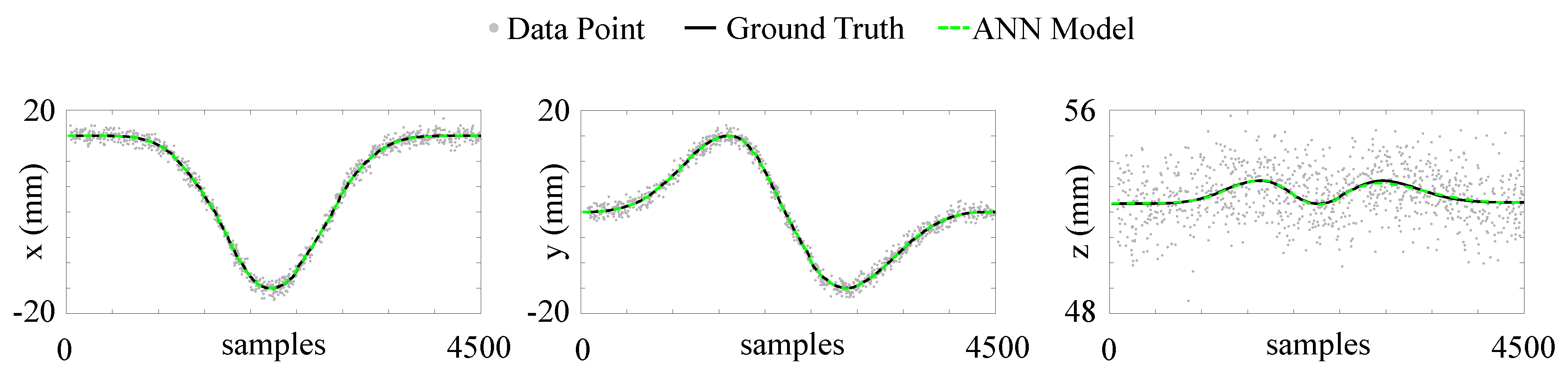
3.1. Robot Modelling

To build the model of the robot as presented in Section 2.1, a similar process to the one that would be applied on the real system is carried out. The robot is commanded to follow a specified path, which in this case is set to be a circumference with a radius of 15 mm . All measurements are referred to the robot base frame. The simulated kinematics of the robot is obtained through standard Denavit-Hartenberg convention [35]. This model is then used to compute the motor values to command to the robot to follow the path. In the mean time, the end-effector tip position is collected from the simulator. Gaussian noise with zero mean and standard deviation of 1 mm for each Cartesian component is added. In total, the dataset consisted of 30,000 points.
The learning method is then used to learn the simulated kinematics and the mapping from motor values to end-effector tip position from the recorded data. The simulated kinematics is also used to have a ground truth for the learned model and evaluate its performance. Being each position component independent on each other, three different neural networks are employed. In this work, all three networks have a similar structure with one input layer (with the input being the 5-dimensional vector of the motor values θ ), one hidden layer, and one output layer (the output being a 1-dimensional vector corresponding to each Cartesian component). For the x , y components satisfying results were obtained with 20 neurons in the hidden layer, whereas for the z component 10 neurons were used. For all the components, the activation function is set to be a sigmoid, which guarantees smoothness and continuity in the computation of network derivatives. Figure 3 shows the results for the offline learned model. The acquired dataset has been randomly divided into three subsets for the training ( 70 % ), validation ( 15 % ), and testing ( 15 % ). The robust approach [31] is able to find a very good model for the data acquired offline, yielding very small errors between the estimated outputs and the ground truths (Table 1).

3.2. Autonomous Tracking

For the control task, the end-effector of the robot is required to follow three different circular paths: one with a radius of 15 mm , such as the one used for training the network; one with radius of 20 mm ; one with radius of 10 mm . Two exploit the redundancy of the system, two subtasks with different priorities are assigned: the primary task is to perform the circle in the x , y directions; the secondary task is to keep the z constant. In this case the z is fixed at 0.050 m. The robot starts from the home configuration and moves to the circle along a straight line. Then it is required to loop around twice. The desired motion time is set to 25 s (5 s for reaching the circle and 20 s for looping) with a sampling time d t = 1 ms . The motor commands are computed as in (3), where P d , 1 is the 2D vector of the desired x , y tip position, P a , 1 the x , y measured components of the tip position, P d , 2 is the z tip position, P a , 2 the measured z component. Since we focused only on path tracking, the desired velocities P ˙ d , 2 , P ˙ d , 2 can be set to 0.
Figure 4 plots the results for tracking the desired paths, whereas Figure 5 shows the absolute errors for each Cartesian component between the ANN expected position and the desired position ( ϵ N N , d ), the expected position and the actual tip position ( ϵ N N , a ), and between the actual and the desired positions ( ϵ a , d ).
For all the three paths, the feedback controller is able to lead to good tracking performance, with small errors between the actual tip position and the desired one. This happens because, despite the modelling errors between the expected network output and the actual tip position, the error at the velocity level is small, and, therefore, feasible for the feedback controller to compensate for (4). The proposed adaptive method also leads to effective tracking, with generally smaller errors, especially in the z direction. The errors in the z direction are higher than those along x , y since the former is given a lower priority. For the adaptation, the retraining set consists of the latest 100 data points and each model for each Cartesian component is re-adapted whenever ( ϵ N N , a ) is greater than a certain threshold, set to 0.5 0.5 1 mm for each component. The threshold for the z is larger, being it a less important task. However, when no adaptation is implemented, the errors between the actual tip position and the ANN expected position are large. The adaptation, instead, ensures minimization also of ϵ N N , a , and, thus, minimizing the risk of instability of the system. Table 2 shows the mean absolute errors ϵ ¯ a , d , ϵ ¯ N N , a in the different cases.
Thanks to the use of a global learning method such as ANN, which allows having more generalizable models compared to local learning methods such as those proposed in [13,16], model adaptation is not always needed, therefore there is not a continuous re-learning of the model. Table 3 shows the number of times each model, for each Cartesian component, was adapted. Due to the adaptation, however, the total time for executing the desired motion tasks is larger than in the case with a simple feedback controller.
The main drawback of a simple feedback controller is that it works well if the model is accurate enough. In surgical robots, however, nonlinear effects such as friction, cable extensions, or even the occurrence of a broken tendon are difficult to predict and compensate for. To validate the effectiveness of the proposed method, we designed a path tracking test where the robot needs to follow the circular path of 15 mm in radius, but with a broken joint (Elbow 1). In this scenario, the joint is considered locked at an angle of 10 . Detecting which joint is not functioning anymore may be challenging or even impossible in a real scenario and, therefore, the system model needs to adapt accordingly. In this case, no information about the broken joint is given, and the controller only receives data about the tip position and the commanded motor values. Figure 6 shows that the proposed method is able to effectively relearn the model and ensure correct execution of the task. Apart from some initial errors, the adaptation is able to converge to an accurate model. When a simple feedback controller is used, instead, the system becomes unstable and fails the tracking task, due to the unmodelled errors. When the adaptation is activated, the mean absolute errors result to be ϵ ¯ a , d = 0.006 0.006 1.625 mm and ϵ ¯ N N , d = 0.208 0.215 1.639 mm , proving the capabilities of the approach to guarantee correct path tracking. Again the errors along z are higher since it is a lower priority task. In this case, the model for the x component adapted 171 times, the one for the y component 265 times, and the one for the z component 28 times. Larger number of adaptations occur due to the unpredicted system behaviour.

3.3. Teleoperation

To further prove the capabilities of the proposed method, a teleoperation test is also performed. This test serves for two purposes. On one hand, surgical robots are usually teleoperated and, therefore, the adaptation must be fast and accurate enough to allow the robot to follow the master commands. On the other hand, through teleoperation it was possible to generate paths completely different from the training one, which might happen due to tissue deformations. Also in this case the primary task is following the path in the x , y Cartesian space. The same thresholds and memory size of the autonomous tracking are used.
Figure 7a shows the results. Thanks to the fast model adaptation, there is very little lag between the commanded motion and the executed one. Moreover, the model adaptation proved effective and able to allow the system to compensate for the errors and follow the desired path with high accuracy resulting in ϵ ¯ a , d = 0.144 0.214 3.922 mm and ϵ ¯ N N , d = 0.248 0.277 3.616 mm . Again, errors in the z direction are higher, but just because this task is not as important as the tracking in the x , y plane.
If larger and faster motions were commanded, the adaptation would take longer. However, in surgical environments, motions are usually slow, making the use of this method in such operations feasible.
Also for the teleoperation case, a test with a broken joint was conducted. Again, the adaptive method allows effectively relearning the model and guarantee safe and correct task execution, as shown in Figure 7b. The mean absolute errors result to be ϵ ¯ a , d = 0.087 0.236 3.185 mm and ϵ ¯ N N , d = 0.209 0.239 3.076 mm . Due to the reduction of redundancy and dexterity for the broken joint, the tracking errors are generally higher.

4. Discussion

The simulation results showed the capabilities of the proposed approach in re-adapting the model of the surgical tool online, improving system’s stability and tracking performance. However, the speed of the adaptation still depends on different parameters, such as the size of the memory chosen, the complexity of the neural network, and the learning algorithm. Having a large dataset for retraining may allow building a better global model, whereas if a short memory is used, the proposed approach may be considered more like a local learning method. A network with many layers and neurons may also better learn a global model, yet it highly increases the computational cost for the adaptation. The algorithm for adaptation also has impact on the time it takes the adaptation to minimize the errors in the dataset. Levenberg-Marquardt algorithm was chosen because it is a generalization of the gradient descend method, it is fast, and allows specifying the damping factor μ , which affects the rate of change of the network weights. Moreover, in this work, the proposed approach was tested only in simulation. To better compensate for modelling errors due to the nonlinearities in the real system, a more complex network architecture may be needed, with more layers and neurons.
Finally, another point to consider is that the proposed adaptation relies only on the measured tip position and on the commanded motor values. The motor values can be directly measured from the motor encoders, whereas, for the tip position external sensors such as electromagnetic trackers or the endoscopic camera need to be used. The accuracy of the adaptation therefore depends on the accuracy of the measurements.

5. Conclusions

One of the major challenges that still limits the use of autonomous (or little supervised) surgical robots is proper modelling and control of these systems. The nonlinearities in the actuation, the highly articulated design, and the unstructured surgical environments require complex modelling techniques and control strategies to guarantee safety and accuracy. An inaccurate model may lead to system instability and improper control, causing serious traumas to the patients. In this work, we presented an approach to control a redundant surgical robot, consisting in learning the forward kinematic model of the robot by means of a global learning method such as ANN. The forward kinematic model is learned because it allows having access to the robot Cartesian Jacobian and, thus, exploit effectively the redundancies of the system.
As for the chosen modelling method, ANN have been chosen for different reasons. Firstly, they allow modeling complex functions; secondly, their parametric nature makes it easy and fast to compute the robot Jacobian; thirdly, being global methods, they reduce the amount of model adaptation and increase the reliability in case data cannot be collected and used to learn the model online. Most of the state-of-the-art works, instead, focus on learning the inverse kinematics of surgical robots, therefore, given the desired tip position, the machine learning algorithm is employed to directly retrieve the corresponding joint or motor values. Consequently, this does not allow for solving the motion task as an optimal control problem, thus neglecting the possibility to execute prioritized subtasks. In an highly articulated robot, such as the Micro-IGES, however, exploiting the redundancies can be beneficial to improve the versatility of the system and execute a desired task more safely.
In our approach, the kinematic model of the robot is first learned offline. Having an accurate model allows effectively tracking a desired path even with a simple feedback controller. However, when unpredicted changes in the system occur, such as a broken tendon, a feedback controller may lead to system instability and failure to execute the task. The proposed adaptive method, instead, proved its effectiveness in allowing the model to quickly adapt to a changing environment. Results show that the precision achieved in tracking the path is very high, even when unknown paths need to be tracked, as in the case of teleoperation.
Future work will focus on implementing the proposed method on a real surgical robotic tool, where the nonlinear effects of the tendon-driven transmission are difficult to model and highly unpredictable. As a matter of fact, the simulation used here does not consider nonlinear effects such as friction or tendon elongation and slack, which are common in tendon-driven surgical robots and which can cause inaccuracies in the model and in the control. These effects are configuration dependent and a fixed offline model may not be accurate enough to achieve the required precision. The proposed online model adaptation may be able to compensate for the modelling errors, improving the tracking performance.

Supplementary Materials

The following are available online at https://www.mdpi.com/2218-6581/9/3/68/s1, Video S1: video_AdaptiveModelling.mp4.

Author Contributions

Conceptualization, methodology, software, validation, writing, F.C.; supervision and proofreading, P.K., G.P.M. All authors have read and agreed to the published version of the manuscript.

Funding

This research received no external funding.

Conflicts of Interest

The authors declare no conflict of interest.

References

  1. Yip, M.; Das, N. Robot Autonomy for Surgery. arXiv 2017, arXiv:1707.03080. [Google Scholar]
  2. Do, T.N.; Tjahjowidodo, T.; Lau, M.W.; Phee, S.J. Nonlinear friction modelling and compensation control of hysteresis phenomena for a pair of tendon-sheath actuated surgical robots. Mech. Syst. Signal Process. 2015, 60, 770–784. [Google Scholar] [CrossRef]
  3. Ismail, M.; Ikhouane, F.; Rodellar, J. The Hysteresis Bouc-Wen Model, a Survey. Arch. Comput. Methods Eng. 2009, 16, 161–188. [Google Scholar] [CrossRef]
  4. Do, T.N.; Tjahjowidodo, T.; Lau, M.W.; Yamamoto, T.; Phee, S.J. Hysteresis modeling and position control of tendon-sheath mechanism in flexible endoscopic systems. Mechatronics 2014, 24, 12–22. [Google Scholar] [CrossRef]
  5. Do, T.N.; Tjahjowidodo, T.; Lau, M.W.S.; Phee, S.J. Performance Control of Tendon-Driven Endoscopic Surgical Robots With Friction and Hysteresis. arXiv 2017, arXiv:1702.02063. [Google Scholar]
  6. Tjahjowidodo, T.; Zhu, K.; Dailey, W.; Burdet, E.; Campolo, D. Multi-source micro-friction identification for a class of cable-driven robots with passive backbone. Mech. Syst. Signal Process. 2016, 80, 152–165. [Google Scholar] [CrossRef]
  7. Palli, G.; Borghesan, G.; Melchiorri, C. Modeling, identification, and control of tendon-based actuation systems. IEEE Trans. Robot. 2012, 28, 277–290. [Google Scholar] [CrossRef]
  8. Do, T.N.; Tjahjowidodo, T.; Lau, M.W.; Phee, S.J. An investigation of friction-based tendon sheath model appropriate for control purposes. Mech. Syst. Signal Process. 2014, 42, 97–114. [Google Scholar] [CrossRef]
  9. Xu, K.; Simaan, N. Actuation compensation for flexible surgical snake-like robots with redundant remote actuation. In Proceedings of the 2006 IEEE International Conference on Robotics and Automation, Orlando, FL, USA, 15–19 May 2006; pp. 4148–4154. [Google Scholar] [CrossRef]
  10. Nguyen-Tuong, D.; Peters, J. Model learning for robot control: A survey. Cogn. Process. 2011, 12, 319–340. [Google Scholar] [CrossRef]
  11. Reinhart, R.; Shareef, Z.; Steil, J.; Reinhart, R.F.; Shareef, Z.; Steil, J.J. Hybrid Analytical and Data-Driven Modeling for Feed-Forward Robot Control. Sensors 2017, 17, 311. [Google Scholar] [CrossRef]
  12. Yu, B.; Fernández, J.D.G.; Tan, T. Probabilistic Kinematic Model of a Robotic Catheter for 3D Position Control. Soft Robot. 2019, 6, 184–194. [Google Scholar] [CrossRef] [PubMed]
  13. Salaün, C.; Padois, V.; Sigaud, O. Control of redundant robots using learned models: An operational space control approach. In Proceedings of the 2009 IEEE/RSJ International Conference on Intelligent Robots and Systems, St. Louis, MO, USA, 10–15 October 2009; pp. 878–885. [Google Scholar] [CrossRef] [Green Version]
  14. Thuruthel, T.G.; Falotico, E.; Cianchetti, M.; Laschi, C. Learning Global Inverse Kinematics Solutions for a Continuum Robot. In CISM International Centre for Mechanical Sciences, Courses and Lectures; Springer International Publishing: Cham, Switzerland, 2016; pp. 47–54. [Google Scholar] [CrossRef]
  15. Xu, W.; Chen, J.; Lau, H.Y.; Ren, H. Data-driven methods towards learning the highly nonlinear inverse kinematics of tendon-driven surgical manipulators. Int. J. Med Robot. Comput. Assist. Surg. 2017, 13, e1774. [Google Scholar] [CrossRef] [PubMed]
  16. Yip, M.C.; Sganga, J.A.; Camarillo, D.B. Autonomous Control of Continuum Robot Manipulators for Complex Cardiac Ablation Tasks. J. Med. Robot. Res. 2017, 2, 1750002. [Google Scholar] [CrossRef]
  17. Kim, C.; Ryu, S.C.; Dupont, P.E. Real-time adaptive kinematic model estimation of concentric tube robots. In Proceedings of the IEEE International Conference on Intelligent Robots and Systems, Hamburg, Germany, 28 September–2 October 2015; pp. 3214–3219. [Google Scholar] [CrossRef] [Green Version]
  18. Zhang, D.; Wei, B. A review on model reference adaptive control of robotic manipulators. Annu. Rev. Control 2017, 43, 188–198. [Google Scholar] [CrossRef]
  19. Hornik, K. Approximation capabilities of multilayer feedforward networks. Neural Netw. 1991, 4, 251–257. [Google Scholar] [CrossRef]
  20. Cybenko, G. Approximation by superpositions of a sigmoidal function. Math. Control Signals Syst. 1989, 2, 303–314. [Google Scholar] [CrossRef]
  21. Bishop, C. Neural Networks Pattern Recognit; Neural Networks for Pattern Recognition: New York, NY, USA, 1995. [Google Scholar]
  22. Coppelia Robotics. Available online: http://www.coppeliarobotics.com (accessed on 31 July 2014).
  23. Shang, J.; Leibrandt, K.; Giataganas, P.; Vitiello, V.; Seneci, C.A.; Wisanuvej, P.; Liu, J.; Gras, G.; Clark, J.; Darzi, A.; et al. A Single-Port Robotic System for Transanal Microsurgery—Design and Validation. IEEE Robot. Autom. Lett. 2017, 2, 1510–1517. [Google Scholar] [CrossRef]
  24. Murray, R.M.; Li, Z.; Sastry, S. A Mathematical Introduction to Robotic Manipulation; CRC Press: Boca Raton, FL, USA, 1994. [Google Scholar]
  25. Leibrandt, K.; Wisanuvej, P.; Gras, G.; Shang, J.; Seneci, C.A.; Giataganas, P.; Vitiello, V.; Darzi, A.; Yang, G.Z. Effective Manipulation in Confined Spaces of Highly Articulated Robotic Instruments for Single Access Surgery. IEEE Robot. Autom. Lett. 2017, 2, 1704–1711. [Google Scholar] [CrossRef]
  26. Cursi, F.; Malzahn, J.; Tsagarakis, N.; Caldwell, G. An online interactive method for guided calibration of multi-dimensional force/torque transducers. In Proceedings of the IEEE/RAS International Conference on Humanoid Robotics, Birmingham, UK, 15–17 November 2017; pp. 398–405. [Google Scholar]
  27. Hawkins, D.M. Identification of Outliers; Springer: Berlin, Germany, 1980. [Google Scholar]
  28. Aggarwal, C.C. Outlier Analysis; Springer: Berlin, Germany, 2017. [Google Scholar] [CrossRef]
  29. Khamis, A.; Ismail, Z.; Haron, K.; Mohammed, A. The Effects of Outliers Data on Neural Network Performance. J. Appl. Sci. 2005, 8, 1394–1398. [Google Scholar]
  30. Liano, K. Robust error measure for supervised neural network learning with outliers. IEEE Trans. Neural Netw. 1996, 7, 246–250. [Google Scholar] [CrossRef]
  31. Cursi, F.; Yang, G.Z. A Novel Approach for Outlier Detection and Robust Sensory Data Model Learning. In Proceedings of the 2019 IEEE/RSJ International Conference on Intelligent Robots and Systems (IROS), Macau, China, 3–8 November 2019; pp. 4250–4257. [Google Scholar] [CrossRef]
  32. Sciavicco, L.; Siciliano, B. A Solution Algorithm to the Inverse Kinematic Problem for Redundant Manipulators. IEEE J. Robot. Autom. 1988, 4, 403–410. [Google Scholar] [CrossRef]
  33. Chiaverini, S.; Oriolo, G.; Walker, I.D. Kinematically Redundant Manipulators. In Springer Handbook of Robotics; Springer: Berlin/Heidelberg, Germany, 2008; pp. 245–268. [Google Scholar] [CrossRef]
  34. Moré, J.J. The Levenberg-Marquardt Algorithm: Implementation and Theory; Springer: Berlin/Heidelberg, Germany, 1978; pp. 105–116. [Google Scholar] [CrossRef] [Green Version]
  35. Siciliano, B.; Sciavicco, L.; Villani, L.; Oriolo, G. Robotics; Springer: London, UK, 2009. [Google Scholar] [CrossRef]
Figure 1. Micro-IGES surgical tool: (a) Computer Aided design (CAD) model; (b) kinematic model. The shaft provides the Roll and Translation DOFs; Elbow 1 and Elbow 2 result from the mechanical coupling of two pairs of joints; the jaws provide the Wrist Yaw and gripping DOFs about the same rotation axis.
Robotics 09 00068 g001
Figure 2. Flow chart for the online model adaptation and trajectory tracking.
Robotics 09 00068 g002
Figure 3. Results of the offline modelling of the robot kinematics on the test set for each Cartesian component. The ground truth is obtained form the analytical model used for the simulation and the data points are drawn from a Gaussian distribution with zero mean and standard deviation of 1 mm for each component.
Robotics 09 00068 g003
Figure 4. Comparison of the results for tracking the desired paths of 15 mm , 10 mm , 20 mm in radius with and without online model adaptation.
Robotics 09 00068 g004
Figure 5. Absolute position errors ϵ N N , d , ϵ a , d , and ϵ N N , a for the strategies without and with model adaptation in tracking the desired paths: (a) circumference of 15 mm in radius; (b) circumference of 10 mm in radius; (c) circumference of 20 mm in radius. The dashed red line is the threshold triggering the adaptation.
Robotics 09 00068 g005aRobotics 09 00068 g005b
Figure 6. Absolute position errors ϵ N N , d , ϵ a , d , and ϵ N N , a and Cartesian path for the autonomous tracking with broken joint without (top) and with (bottom) model adaptation. The dashed red line is the threshold triggering the adaptation. Without the model adaptation, after about 5 s the system becomes unstable and fails to track the path.
Robotics 09 00068 g006
Figure 7. Absolute position errors ϵ N N , d , ϵ a , d , and ϵ N N , a and Cartesian path for the teleoperation tracking with model adaptation, when the robot is: (a) without broken joint; (b) with broken joint. The dashed red line is the threshold triggering the adaptation.
Robotics 09 00068 g007
Table 1. Root Mean Squared Errors (RMSE) between the ground truth and the offline ANN model for each Cartesian component of the end-effector position.
RMSE (mm)
Train Validation Test
x0.0400.0400.040
y0.0190.0180.019
z0.0340.0350.034
Table 2. Mean absolute errors for the tracking tests.
15 mm Radius10 mm Radius20 mm Radius
w/ Adapt w/o Adapt w/ Adapt w/o Adapt w/ Adapt w/ o Adapt
ϵ ¯ N N , d ( mm ) x0.2065.3500.2211.1560.19210.022
y0.1822.6480.1921.8700.1942.471
z0.5835.4780.5193.6060.6787.605
ϵ ¯ a , d ( mm ) x0.0060.0070.0040.0030.0080.009
y0.0060.0060.0040.0040.0080.008
z0.4240.9300.2830.9180.7140.915
Table 3. Number of model adaptations for the tracking test on the paths of 15 mm , 10 mm , 20 mm radius.
15 mm10 mm20 mm
x422222
y291616
z532739

