Article

Inverse Kinematics with a Geometrical Approximation for Multi-Segment Flexible Curvilinear Robots

1
Department of Biomedical Engineering, National University of Singapore, Singapore 119077, Singapore
2
National University of Singapore Suzhou Research Institute, Suzhou 215125, China
*
Author to whom correspondence should be addressed.
Robotics 2019, 8(2), 48; https://doi.org/10.3390/robotics8020048
Submission received: 1 April 2019 / Revised: 31 May 2019 / Accepted: 12 June 2019 / Published: 19 June 2019
(This article belongs to the Special Issue Robotics, Imaging, and Navigation Sensors for Medical Applications)

Abstract

:
Despite research related to flexible or continuum curvilinear robots, there lacks a common simulation tool for continuum robots, which are unlike rigid robots. Thus, in this paper, a robotics toolbox is utilized to model a wire-driven flexible manipulator as one of the continuum robots. Constant curvature property can enable the robotics toolbox to represent the flexible manipulator and validate its kinematics. Moreover, because the closed-form inverse kinematics methods developed previously for real-time control conceded limitations in modeling some continuum robots, we hereby develop an inverse kinematics method for the wire-driven flexible manipulator which can provide fast and reliable inverse results. Experimental results showed that geometrical information offered a stable starting point for the proposed inverse kinematics algorithm. Moreover, the first and second derivatives of a fitness function further contributed to a fast-converging solution within a few microseconds. Lastly, for the potential feasibility of an active compliance controller without physical force/torque sensors, a reaction torque observer was investigated for a flexible manipulator with direct drive mechanisms.

1. Introduction

To improve efficiency and curvilinear accessibility in medical, service, and industry fields, new curvilinear robotic technologies called flexible or continuum robots have emerged. Unlike rigid robots, continuum robots [1] have inherent compliance, curvilinear accessibility, are relatively lightweight, and have high dexterity, which can be suitable for unstructured or confined environments such as the human body [2,3]. Moreover, these continuum robots are typically operated by shape memory alloy (SMA) [4], electroactive polymer (EAP) [5], pneumatic artificial muscle (PAM) [6], piezoelectric ceramic (PZT) [7], electric motors with wires or tendon transmissions [8], combinations of concentric tubes [9], etc. Then, kinematics and dynamic modeling for these kinds of new hardware designs and actuation methods are developed for operation in various applications.
Historically, the work [10] suggested a modal approach for hyper-redundant robots. Moreover, an Air-OCTOR robot inspired by an element trunk suggested the conventional Denavit–Hartenberg (D-H) method for kinematic analysis of the continuum robot [11]. Closed-form inverse kinematics (IK) provided a geometrical analysis with constant curvature property [12].
On the other hand, numerical optimization techniques are generally applied to solve inverse kinematics for the continuum robot [13,14,15,16,17,18]. As an example, Iqbal et al. [13] suggested the use of interval analysis to deal with uncertainties in the IK. Recently, to deal with nonlinearities of a continuum arm’s hardware, machine learning methods were also applied to learn the IK of a tendon-driven manipulator [19]. IK studies for continuum robots are listed in Table 1 and well-organized summaries of the kinematics of the continuum robot were reported in [6,20].
This paper describes a new mathematical formulation for a wire-driven flexible manipulator (WDM) as one of the continuum robots for forward and especially inverse kinematics, as well as utilization of the MATLAB robotics toolbox [21]. For real-time control of the continuum robot, fast and accurate solution of the IK is generally required. Even though the previous closed-form IK method [12] is quite suitable for real-time control, it could not be applied to some types of continuum robots, as will be explained later, since the solution may be unreliable near singularities [21]. Moreover, some literature reported that the order of tens of milliseconds, as shown in Table 1, was required to solve an IK problem by iterative numerical methods [13,15,17]. Because the computation time might be an average value and it might be affected by the complexity of the continuum robot’s design, such as multi-section, the worst-case might jeopardize control performance. In this paper, to reduce the time required to solve the IK problem, a geometrical approximation is used for an initial guess of numerical optimization. The closed-form IK method did not provide an accurate solution but gave an approximate bending angle value in the WDM. Thus, this proper starting point enables the reduction of convergent time and even avoids local optima. The first and second derivatives of a fitness function are also derived for fast and accurate computation. As a result, the convergent rate of the proposed IK algorithm is approximately 100 times faster than the previous ones, as will be shown in the experiment section.
Another contribution of this paper is to suggest the utilization of the robotics toolbox [21] as a common tool for continuum robots’ kinematic analysis. Although there is a lot of work on continuum robots, there is no common continuum robot analysis tool to compare with rigid robots, which may make it difficult for beginners to enter this field. Thanks to the constant curvature property, the kinematic behavior of a continuum robot can be easily visualized by the robotics toolbox, which can help to understand it deeply, save time to simulate it, and validate derived kinematic equations.
Furthermore, so-called intrinsic force sensing [22] and active compliance controls such as force control [23] and impedance control [24] have been recently studied in continuum robots. As a preliminary step for active compliance controls, a reaction torque observer (ROB) at a proximal side of the WDM with direct drive [25] is briefly introduced without physical force/torque sensors. Its potential feasibility for compliance control is also investigated.
The remaining parts of the paper are organized as follows: Section 2 briefly reviews a wire-driven flexible manipulator—D-H parameters of the WDM are derived and the MATLAB robotics toolbox [21] is used to represent the WDM; Section 3 analyzes the closed-form IK method and proposes an IK algorithm which gives fast and accurate results; Section 4 introduces the ROB for the WDM; Section 5 shows the results of the proposed IK algorithm, comparing with the closed IK method and responses of the ROB in the WDM; and Section 6 concludes the paper.

2. WDM’s Inverse Kinematics with the Robotics Toolbox

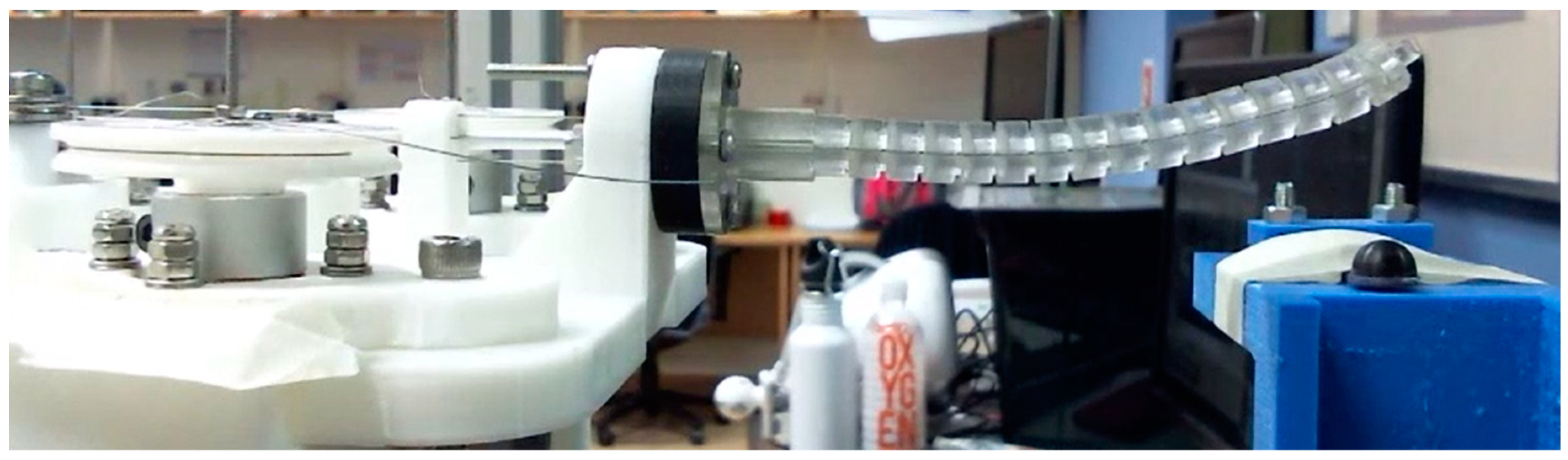
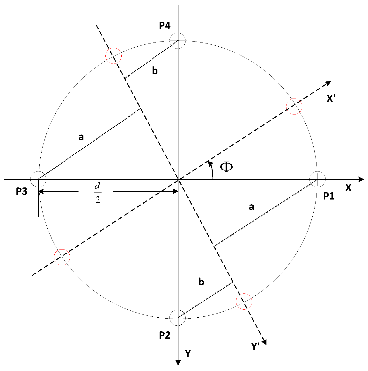
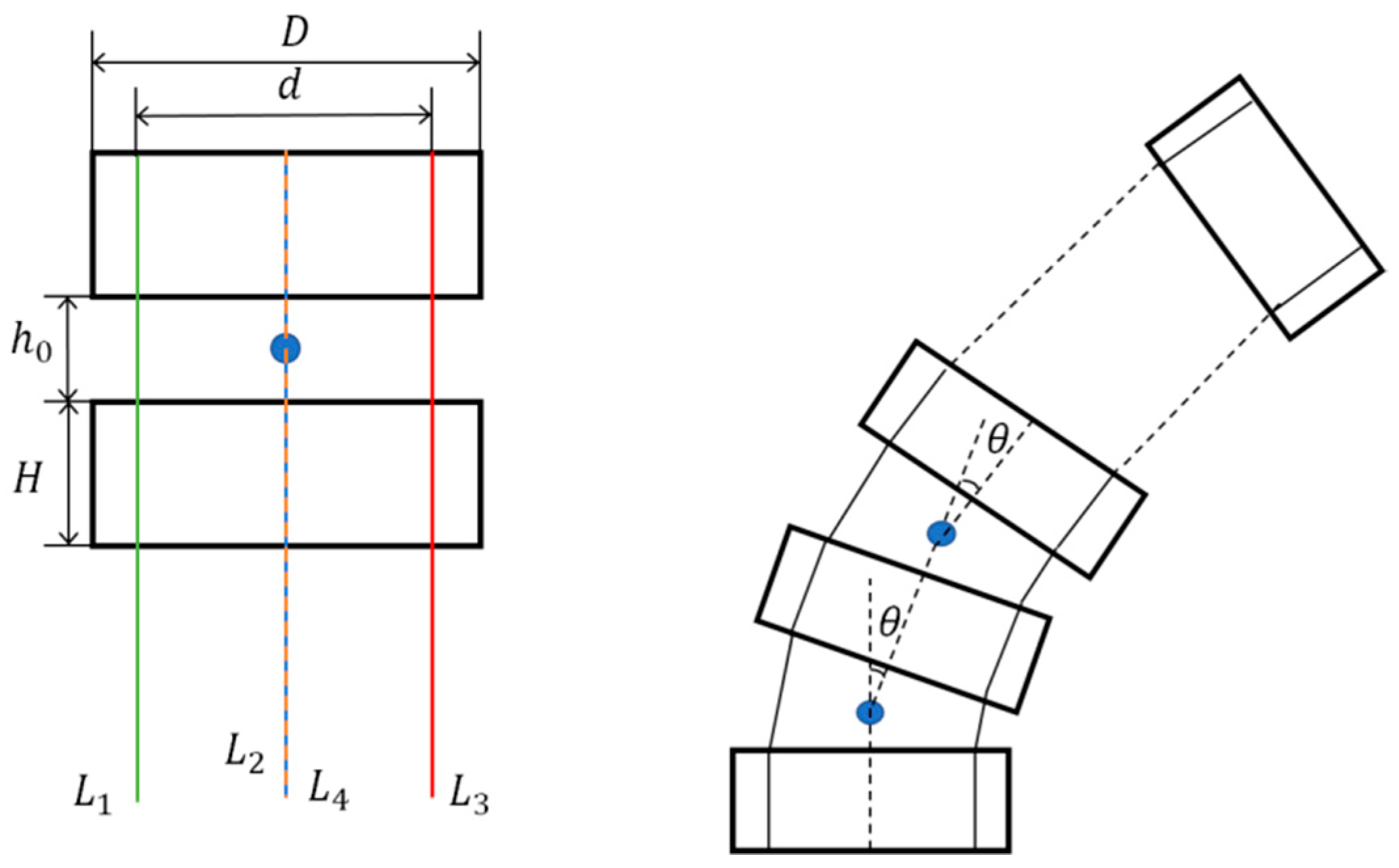
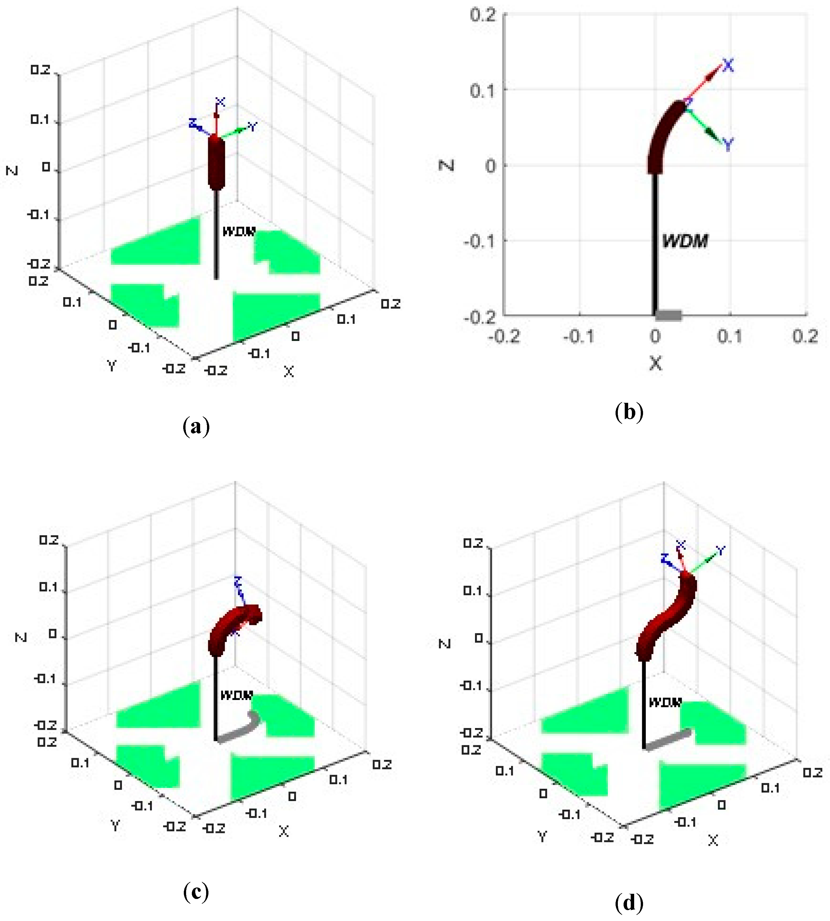
2.1. Review of the WDM

Figure 1 shows a wire-driven serpentine manipulator, a type of WDM inspired by a snake and an octopus’ arm [26]. The mechanism design of this system can be referred to in [25]. In this section, the kinematics of the WDM are not only briefly reviewed but also revised to utilize the robotics toolbox [21].
At first, the kinematics of the WDM can be defined as two stages [8]: from actuator space to configuration space ( f 1 ) , and from configuration space to task space ( f 2 ) . Although the flexible WDM can be considered as the continuum robot with its constant curvature property, it can be modeled by joint and link compositions for simplicity of the kinematic analysis. The definition of design parameters and the illustration of the configuration (individual bending angle θ and rotation angle Φ ) can be referred to in Figure 2 and Figure 3. By referring to [26] in Figure 2, each wire length L i ,   i = 1 , 2 , 3 , 4 can be obtained as
L 1 = L 0 2 N ( a sin θ 2 + h 0 sin 2 θ 4 ) L 2 = L 0 2 N ( b sin θ 2 + h 0 sin 2 θ 4 ) L 3 = L 0 + 2 N ( a sin θ 2 h 0 sin 2 θ 4 ) L 4 = L 0 + 2 N ( b sin θ 2 h 0 sin 2 θ 4 ) }
where a = d 2 cos Φ , b = d 2 sin Φ , L 0 is the initial wire lengths at rest state, N is the number of joints of the manipulator and h 0 is the spacing of the two adjacent links at rest state.
Now, based on the above equations, f 1 ’s kinematic relationships can be derived as follows:
Rotation angle Φ
Φ = a t a n 2 ( Δ L 2 , Δ L 1 )
Bending angle Θ
Θ = ( N + 1 ) θ = 2 ( N + 1 ) s i n 1 ( Δ L 1 2 + Δ L 2 2 2 N d )
where Δ L 1 = L 3 L 1 and Δ L 2 = L 4 L 2 .
Then, the position of the WDM can be easily calculated from Figure 4. Suppose that an origin o 0 is placed on the first joint and an origin o N + 1 is located on the center of the WDM’s tip. The 3D tip position can be easily calculated as
X N + 1 = { l ( i = 1 N + 1 sin ( i θ ) ) } cos Φ Y N + 1 = { l ( i = 1 N + 1 sin ( i θ ) ) } sin Φ Z N + 1 = l ( i = 1 N + 1 cos ( i θ ) ) }
where l is the link length of the rigid manipulator. Applying the Dirichlet kernel and the Lagrange’s trigonometric identities, (4) can be rewritten as
X N + 1 = [ l { 1 2 cot θ 2 cos ( ( N + 3 2 ) θ ) 2 sin θ 2 } ] cos Φ Y N + 1 = [ l { 1 2 cot θ 2 cos ( ( N + 3 2 ) θ ) 2 sin θ 2 } ] sin Φ Z N + 1 = l 2 ( 1 + sin ( ( N + 3 2 ) θ ) sin θ 2 ) } .

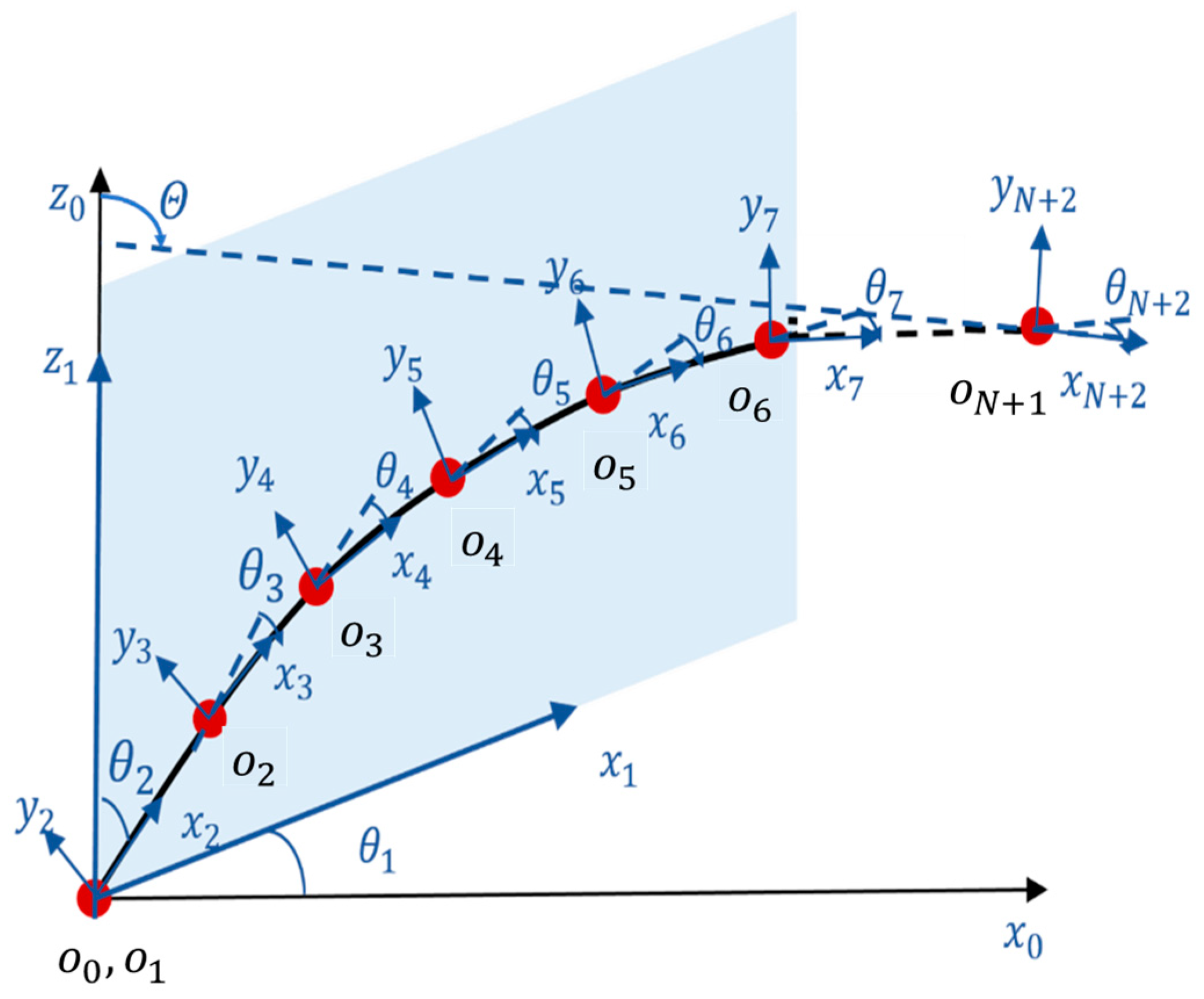
2.2. Denavit–Hartenberg Parameters of the WDM

Based on this assumption and the constant curvature in the bending phase, the WDM can be easily represented by the MATLAB robotics toolbox, a well-known tool for analyzing robots, particularly rigid robots. Figure 3 illustrates the shape of the WDM in the bending phase on the xz plane and D–H coordinates for the WDM can be set, as shown in Figure 4. In addition, the entire Denavit–Hartenberg (D–H) parameters are listed in Table 2. Note that the curved shape of the WDM between two nodes can be approximately represented by a chord equivalent to a link ( l = H + h 0 ) [26] of a rigid manipulator, as shown in Figure 3. Further note that a parameter θ 1 is assigned for the rotation ( Φ ) of the WDM, and an offset π 2 is necessary for the straight shape of the WDM (zero rotation ( Φ ) and bending ( Θ ) angles), as shown in Figure 4.

2.3. Robotics Toolbox for the WDM

With the D-H parameters in Table 2, the WDM can be modeled by the robotics toolbox. Because the WDM has the same parameters from link 2 to link N + 2, D-H parameters can be easily assigned by a link command of the robotics toolbox and a for–loop command even if there are many nodes in the WDM. Note that all θ i parameters in single section arm have the same value except for θ 1 because of the constant curvature property. Further note that an offset angle π 2 must be applied to the link 2 object using an offset member function of the link class in the robotics toolbox. Finally, using the plot member function, the shape of the WDM can be easily visualized. Figure 5 shows different configurations of both one section and two section WDM.
Utilization of the robotics toolbox has two main advantages. The robotics toolbox helps beginners visualize their continuum robot’s configurations and the derived forward kinematic equations can be validated by the forward kinematic member function of the robotics toolbox as a common validation tool. Furthermore, the suggested approach can be easily extended to multi-section robots with proper D–H coordinates.

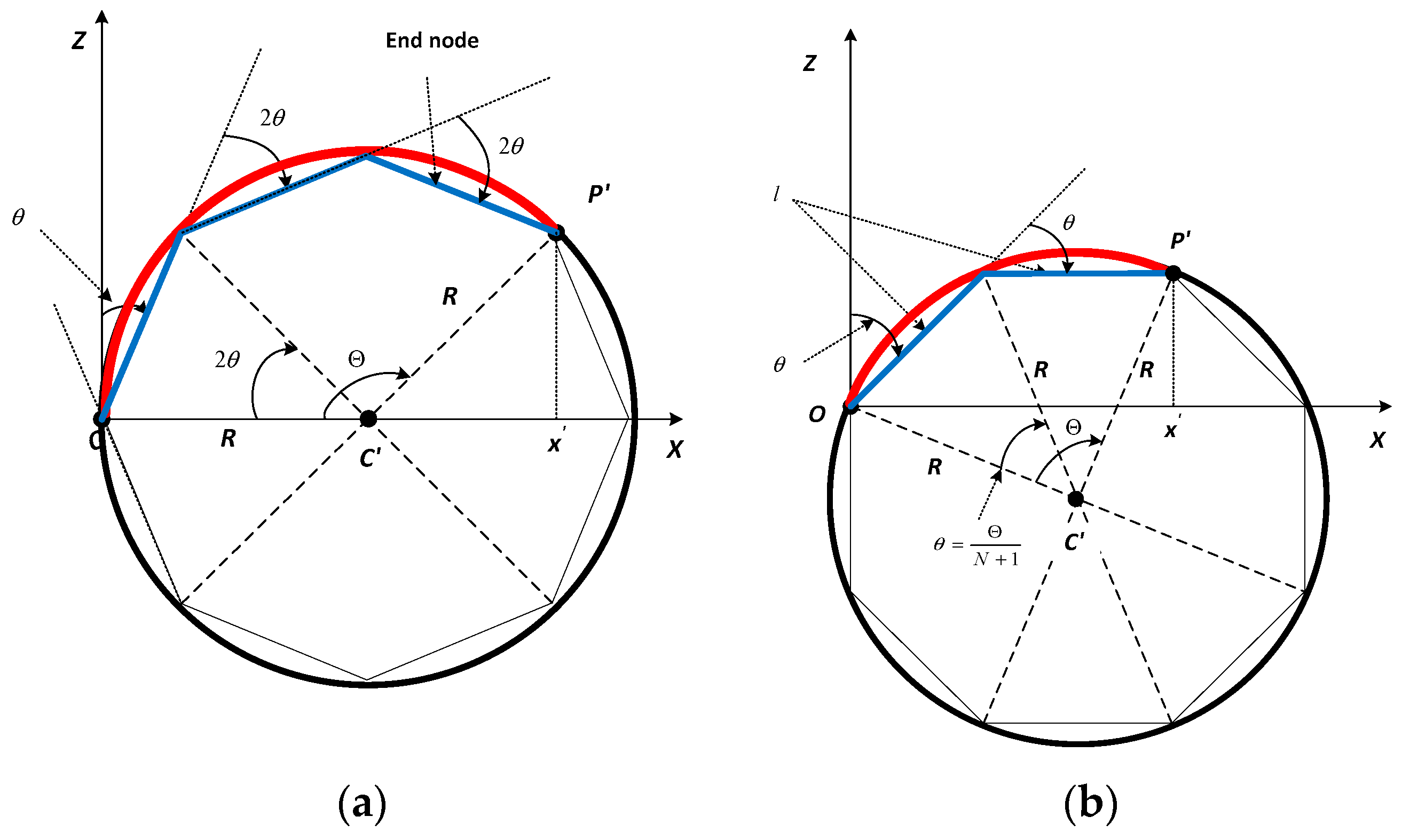
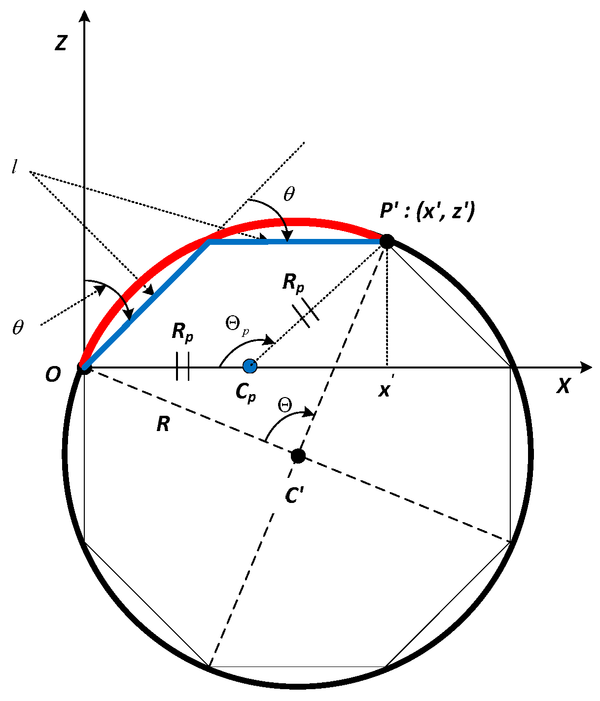
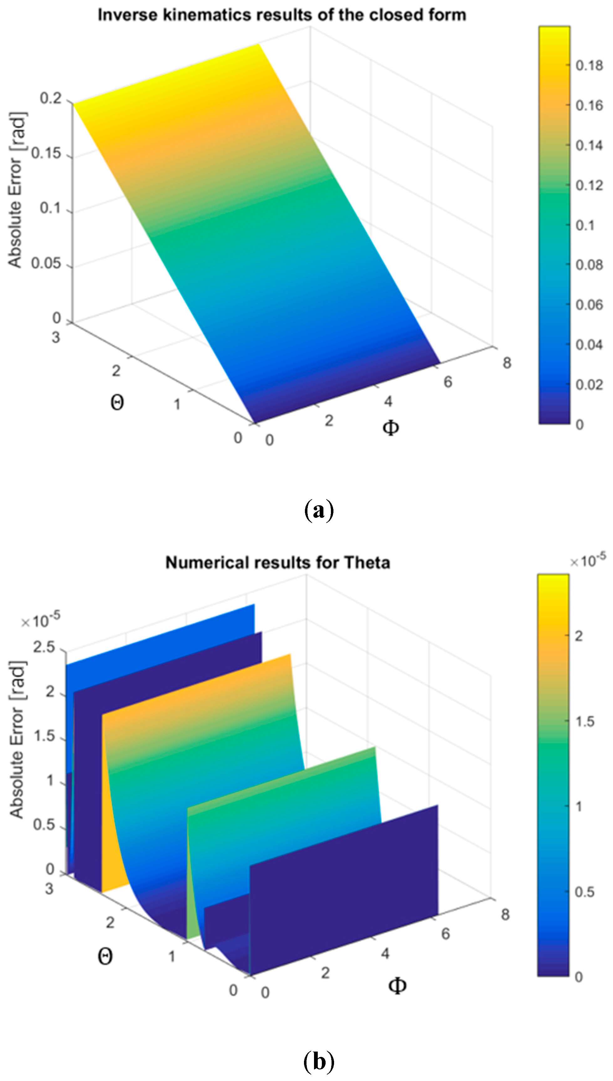
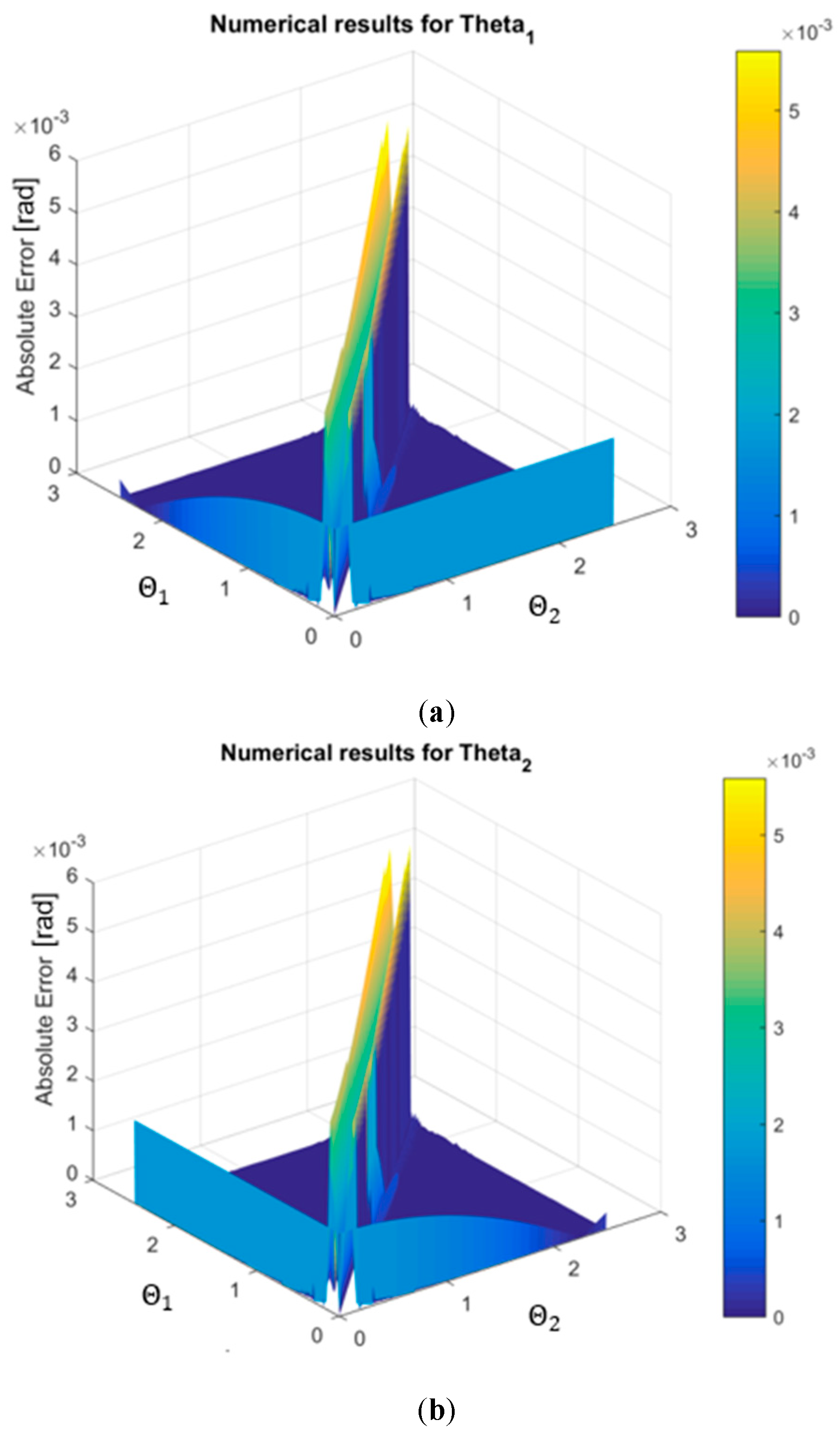
3. Inverse Kinematics with a Geometrical Approximation for the WDM

A fast and reliable IK is very important for real-time control of the WDM with the task space pose command. Even though the closed-form IK [12] for continuum robots was proposed, this method could not be applied to every type of continuum robot because of violation of assumptions. In other words, the closed-form IK method was based on two assumptions: the constant curvature, and the center of the circular arc, which must be located on the x-axis of the base reference after the bending plane is rotated to coincide with the xz plane of the base reference. However, these assumptions are not guaranteed in all cases. To explain these, we chose a regular octagon with a circumcircle, as properties of a regular polygon can help analyze a circular arc’s geometry.
Figure 6a illustrates a WDM with N = 2, showing that the assumption of the center of the circular arc is valid [12]. However, the constant curvature property is not guaranteed because the first bending angle ( θ ) is not the same as the second ( 2 θ ) . On the contrary, if the assumption of the constant curvature is ensured, as shown in Figure 6b, then the other becomes invalid.
From the above analysis, we found that the previous closed-form IK method could not be applied to derive an accurate IK solution from the WDM. Nevertheless, this geometrical information can be used to obtain fast and accurate IK if it is combined with a numerical optimization method because in the numerical analysis, a proper initial guess is generally very important to obtain an accurate solution with fast convergence. Interestingly, the geometrical analysis in Figure 6b can be used to provide a proper initial guess of the bending angle, Θ , as shown in Figure 6, which does not provide a true Θ , but a Θ p . In Figure 7, Rp, Cp, and Θ p represent a pseudo radius, a pseudo center, and a pseudo Θ , respectively. Nevertheless, because the range of the bending angle Θ is generally limited by mechanical constraints and a pseudo Θ p is near a true bending angle, the Θ p can be used as a good initial point to find true Θ in the numerical optimization. Further note that the smaller the bending angle, the more the pseudo Θ p is converged to the true Θ .
In the numerical optimization, to find the accurate bending angle Θ and the corresponding θ with respect to the desired end position (x, y, z), a cost function, which quantifies the tip position error projected on the bending plane, is defined as
f ( θ ) = 1 2 ( e x 2 + e z 2 )
where e x = x X e s t and e z = z Z e s t . x and z are the projected desired position on the x-axis and z-axis, respectively. X e s t = X N + 1 2 + Y N + 1 2 and Z e s t = Z N + 1 are the estimated tip position computed by forward kinematics derived in (5). The optimal bending angle can be found by solving the following constrained optimization problem:
min θ f ( θ )
s . t .   θ L θ θ U
where θ is constrained by the inherent design of the manipulator, with θ L = 0 as the lower bound and θ U as the biggest individual bending angle allowed and θ U = 2 a t a n 2 ( h 0 , D ) .
Moreover, a solution was computed by sequential quadratic programming, which is often used to solve nonlinear optimization problems.
Finally, the displacement of each wire pair of the WDM can be derived as follows
Δ L 1 = L 3 L 1 = 2 N d sin ( θ 2 ) cos ϕ Δ L 2 = L 4 L 2 = 2 N d sin ( θ 2 ) sin ϕ }

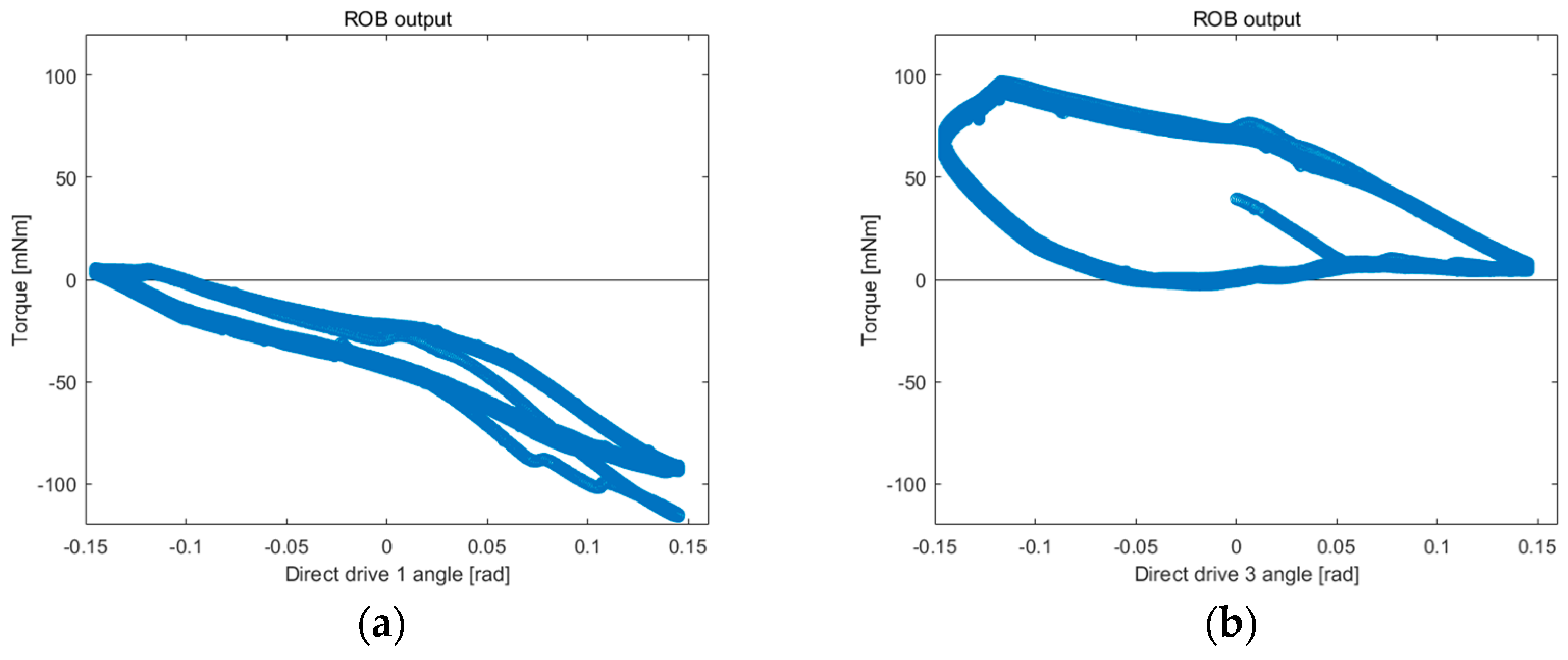
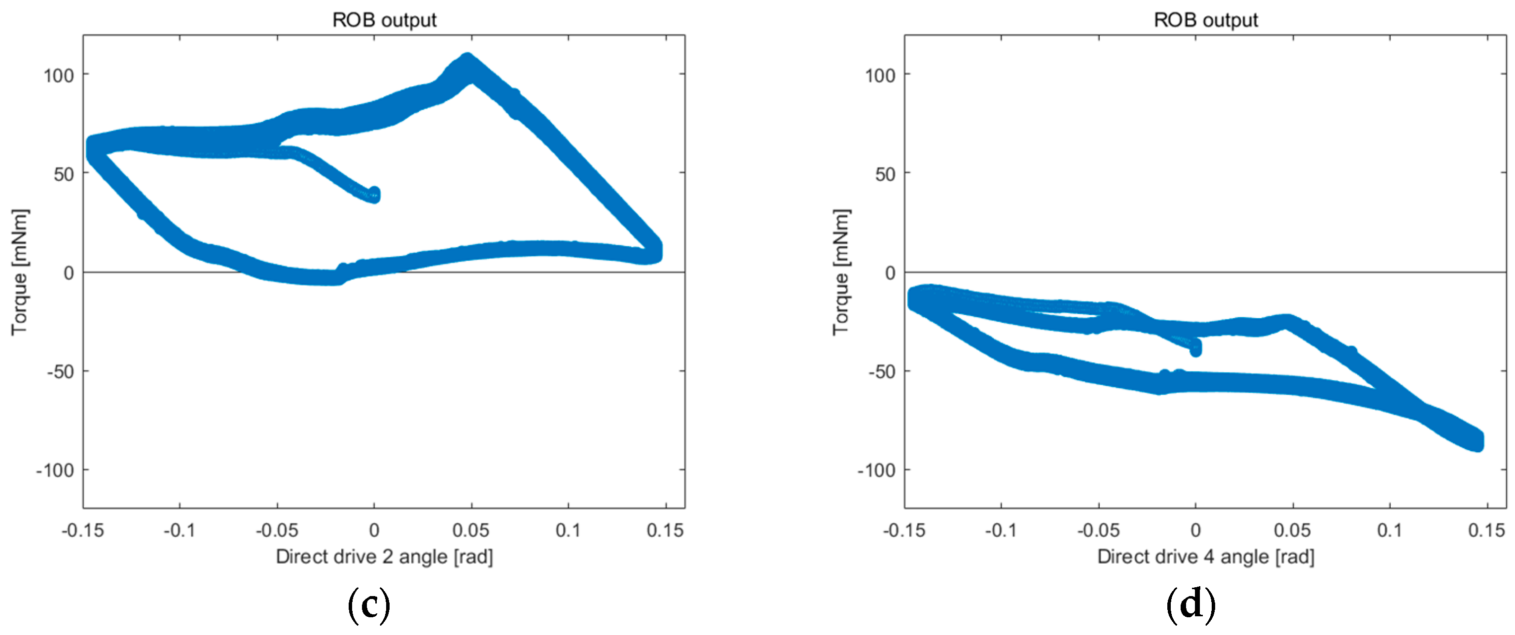
4. Reaction Torque Observer for the WDM
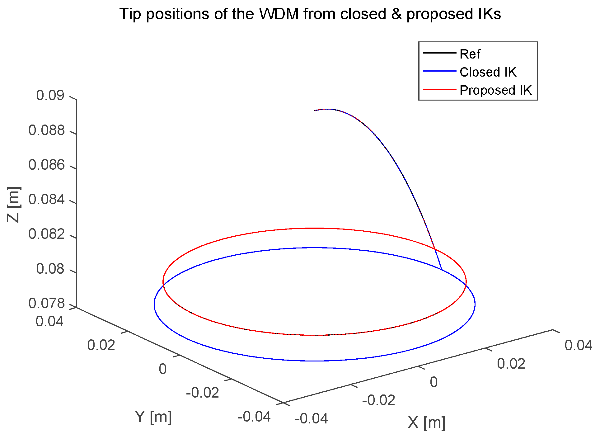
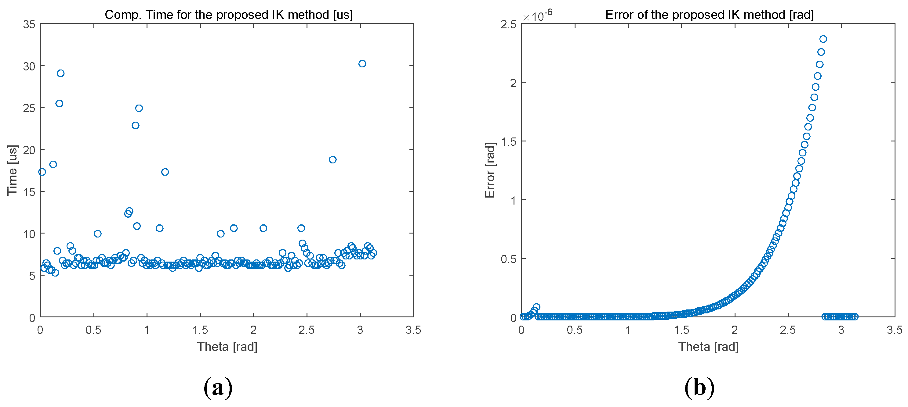
Although there have been a few studies on active compliance control recently, physical force/torque sensors are generally used to perform these controls. In this section, a ROB in the WDM’s actuation space is briefly introduced to estimate external torque at the load side of the WDM’s direct drive. The motion equation of the direct drive can be described as [25]:
T e = J d ω d t + f F r i c ( · ) ω + T e x t
where T e is the actuator torque, which is composed of the controller torque T C and the pretension torque T P , J is the equivalent inertia of the direct drive, ω represents the angular velocity q ˙ , f F r i c ( · ) is the friction torque of the direct drive, and T e x t . is the external torque. Then, using the disturbance observer technique [27], the external torque T e x t can be estimated as
T ^ e x t = L P F ( T C + T P + g J ^ q ˙ ) g J ^ q ˙
where LPF ( · ) = g s + g is a low pass filter, g is the coefficient of the low pass filter, J ^ is the estimated inertia of the direct drive and T e = T c + T P . Note that the friction term in (9) was compensated by a friction compensator [25].

5. Experiments

To validate the proposed IK method, simulation and actual tests were performed by prepared trajectories in task space; these paths are equivalent to the rotation angle Φ with a constant speed after the change of the bending angle Θ from zero to π 4 . These tests were implemented on the WDM, which is composed of a wire-driven flexible arm, the direct drive mechanisms, and the embedded control systems (developed in [25]). The WDM’s mechanical parameters are listed as follows: H = 0.005 m, h 0 = 0.001 m, and N = 14 . Moreover, the dynamics of the direct drive were estimated by system identification experiments [25].
At first, to see the errors of the closed-form IK method in the WDM and verify that this geometrical method can be a good initial point for the optimization, simulations using MATLAB were performed and the results are shown in Figure 8a. As mentioned in section 3, an error ( = t r u e   v a l u e e s t i m a t e d   v a l u e ) is increased as the bending angle Θ increases. Nevertheless, because errors have small ranges and the range of Θ is generally limited by the mechanical constraint, these estimated Θ p can be utilized as a starting point for the numerical optimization. Thus, using MATLAB’s fmincon optimization function, the proposed IK method was simulated, and accurate results were obtained, as shown in Figure 8b. Moreover, Figure 9 shows a comparison of the closed-form and the proposed IK methods in the task space motion control and the kinematic effect may become more critical in multi-section robots.
Since a fast solution to inverse kinematics is even more critical for real-time control of multi-section WDM, we extended the proposed method to a two-section WDM. The two sections are identical and have the same mechanical parameters as the ones used in the previous section. Configuration space parameters for section one and section two are [ Θ 1 ,   Φ 1 ] and [ Θ 2 ,   Φ 2 ] respectively. In the simulation, we consider a specific scenario: Θ 1 = Θ 2 ; in other words, the two sections bend in the same plane. Though this configuration is one of many, it demonstrates the superiority of the proposed algorithm. Simulation results for the absolute error of Θ 1 and Θ 2 are shown in Figure 10a,b, respectively. We can see that the solutions are quite accurate, with absolute errors within 6 × 10⁻³ mm, though the errors at the boundary of Θ 1 and Θ 2 are slightly bigger. Compared to the results of a one-section WDM, the errors for Θ are larger, which is consistent with our expectation.
Secondly, the proposed IK method was implemented on a real WDM testing bed previously designed by us [25] and by C++ in Windows (CPU: i5-4690 3.5 GHz) to compare its convergent rate with other numerical IK methods. For these tests, optimization functions of a dlib library [28] were used. Figure 11 shows the computation times and errors of the proposed IK approach. Although it is not easy to compare with the previous approaches [13,14,15,16,17,18] due to its different kinematic model, the proposed IK method provides accurate and fast (almost 100 times faster) solutions [13,15,17]. Simulation and actual tests of the proposed IK method in the WDM can be found in the supplementary video.
Finally, the designed ROB was applied to the WDM with the same trajectory to investigate the feasibility of the use of the ROB in the WDM. Figure 12 shows the results of the estimated external torques of the four motors of the direct drive system when ROB is applied. Note that motor 1 and 3 and motor 2 and 4 are coupled to each other because of their antagonistic actions. Therefore, when 40 mNm pretensions were applied to prevent a slack problem, ROB outputs for motor 1 and 4 had −40 mNm in the initial equilibrium status. The outputs of the ROB were changed based on the WDM motions and estimated external torques were uniformly repeated in periodic rotation motions of the WDM with constant Θ and Φ [ π , π ] despite high nonlinearities of the flexible arm part. Note that deviated ROB paths, especially in Figure 12a,d, were originated from the WDM’s bending motion (from zero to π 4 ). Small variations of the ROB in the periodic trajectory show that the ROB data can be used to train machine learning algorithms for identifying noncontact/contact status without physical sensors. It can be extended to sensor-less active compliance controls [29], which will be studied in the future.

6. Conclusions

In this paper, the robotic toolbox was introduced to model the WDM. The proposed kinematic analysis and D–H coordinates could enable the visualization of the WDM by the robotics toolbox. Moreover, for real-time control of the WDM, the IK method was proposed. With geometrical approximation and derivatives of the fitness function, the accurate and fast IK algorithm was implemented by C++. Thanks to the very fast convergent rate, the proposed method can even be applied to WDM with multiple bending sections.
In the future, the proposed IK method will be applied to a multi-section WDM and tip position sensing will be utilized to compensate for inaccuracy brought about by improper design and prototyping of the flexible arm will improve position accuracy. Moreover, through the proposed ROB and the flexible arm design, learning algorithms for identifying contact status and sensor-less active compliance controls will be studied.

Supplementary Materials

The following are available online at https://www.mdpi.com/2218-6581/8/2/48/s1.

Author Contributions

Conceptualization, H.R. and S.K.; methodology, S.K.; software, S.K. and W.X.; validation, S.K. and W.X.; data curation, S.K.; writing—original draft preparation, S.K. & W.X.; writing—review and editing, H.R.; visualization, S.K.; supervision, H.R.; project administration, H.R.; funding acquisition, H.R.

Funding

This work is supported by the NMRC Bedside & Bench under grant R-397-000-245-511 and Singapore Academic Research Fund under Grant R397000297114 awarded to Hongliang Ren.

Conflicts of Interest

The authors declare no conflict of interest.

References

  1. Robinson, G.; Davies, J.B.C. Continuum robots—A state of the art. In Proceedings of the IEEE International Conference on Robotics and Automation, Detroit, MI, USA, 10–15 May 1999; pp. 2849–2854. [Google Scholar]
  2. Burgner-Kahrs, J.; Rucker, D.C.; Choset, H. Continuum robots for medical applications: A survery. IEEE Trans. Robot. 2015, 31, 1261–1280. [Google Scholar] [CrossRef]
  3. Kato, T.; Okumura, I.; Song, S.E.; Golby, A.J.; Hata, N. Tendon-driven continuum robot for endoscopic surgery: Preclinical development and validation of a tension propagation model. IEEE/ASME Trans. Mechatron. 2015, 20, 2252–2263. [Google Scholar] [CrossRef] [PubMed]
  4. Kim, Y.; Desai, J.P. Design and kinematic analysis of a neurosurgical spring-based continuum robot using SMA spring actuators. In Proceedings of the IEEE/RSJ International Conference on Intelligent Robots and Systems (IROS), Hamburg, Germany, 28 September–2 October 2015; pp. 1428–1433. [Google Scholar]
  5. Wang, H.; Chen, J.; Lau, H.Y.K.; Ren, H. Motion planning based on learning from demonstration for multiple-segment flexible soft robots actuated by electroactive polymers. IEEE Trans. Robot. Autom. Lett. 2016, 1, 391–398. [Google Scholar] [CrossRef]
  6. Rus, D.; Tolley, M.T. Design, fabrication and control of soft robots. Nature 2015, 521, 467–475. [Google Scholar] [CrossRef] [PubMed] [Green Version]
  7. Su, H.; Cardona, D.C.; Shang, W.; Camilo, A.; Cole, G.A.; Rucker, D.C.; Webster, R.J., III; Fischer, G.S. A MRI-guided concentric tube continuum robot with piezoelectric actuation: A feasibility study. In Proceedings of the IEEE International Conference on Robotics and Automation, Saint Paul, MN, USA, 14–18 May 2012; pp. 1939–1945. [Google Scholar]
  8. Li, Z.; Ren, H.; Chiu, P.W.Y.; Du, R.; Yu, H. A novel constrained wire-driven flexible mechanism and its kinematic analysis. Mechatron. Mach. Theory 2016, 95, 59–75. [Google Scholar] [CrossRef]
  9. Dupont, P.E.; Lock, J.; Itkowitz, B.; Butler, E. Design and control of concentric-tube robots. IEEE Trans. Robot. 2010, 26, 209–225. [Google Scholar] [CrossRef] [PubMed]
  10. Chirikjian, G.S.; Burdick, J.W. A modal approach to hyper-redundant manipulator kinematics. IEEE Trans. Robot. Autom. 1994, 10, 343–354. [Google Scholar] [CrossRef]
  11. Jones, B.A.; Walker, I.D. Kinematics for multisection continuum robots. IEEE Trans. Robot. 2006, 22, 43–55. [Google Scholar] [CrossRef]
  12. Neppalli, S.; Csencsits, M.A.; Jones, B.A.; Walker, I.D. Closed-form inverse kinematics for continuum manipulators. Adv. Robot. 2009, 23, 2077–2091. [Google Scholar] [CrossRef]
  13. Iqbal, S.; Mohammed, S.; Amirat, Y. A guaranteed approach for kinematic analysis of continuum robot based catheter. In Proceedings of the IEEE International Conference on Robotics and Biomimetics (ROBIO), Guilin, China, 19–23 December 2009; pp. 1573–1578. [Google Scholar]
  14. Xu, K.; Simaan, N. Analytic formulation for kinematics, statics, and shape restoration of multibackbone continuum robots via elliptic integrals. J. Mecha. Robot. 2010, 2, 011006. [Google Scholar] [CrossRef]
  15. Godage, I.S.; Guglielmino, E.; Branson, D.T.; Medrano-Cerda, G.A.; Caldwell, D.G. Novel modal approach for kinematics of multisection continuum arms. In Proceedings of the IEEE/RSJ International Conference on Intelligent Robots and Systems, San Francisco, CA, USA, 25–30 September 2011; pp. 1093–1098. [Google Scholar]
  16. Godage, I.S.; Medrano-Cerda, G.A.; Branson, D.T.; Guglielmino, E.; Caldwell, D.G. Modal kinematics for multisection continuum arms. Bioinspir. Biomim. 2015, 10, 035002. [Google Scholar] [CrossRef] [PubMed]
  17. Zhang, Z.; Yang, G.; Yeo, S.H. Inverse kinematics of modular cable-driven snake-like robots with flexible backbones. In Proceedings of the IEEE 5th International Conference on Robotics, Automation and Mechatronics (RAM), Qingdao, China, 17–19 September 2011; pp. 41–46. [Google Scholar]
  18. Amouri, A.; Mahfoudi, C.; Zaatri, A. Contribution to inverse kinematic modeling of a planar continuum robot using a particle swarm optimization. Multiph. Model. Simul. Syst. Des. Monit. 2015, 2, 141–150. [Google Scholar]
  19. Chen, J.; Lau, H.Y.K. Learning the inverse kinematics of tendon-driven soft manipulators with K-nearest neighbors regression and Gaussian mixture regression. In Proceedings of the 2nd International Conference on Control, Automation and Robotics (ICCAR), Hong Kong, China, 28–30 April 2016; pp. 103–107. [Google Scholar]
  20. Webster, R.J., III; Jones, B.A. Design and kinematic modeling of constant curvature continuum robots: A review. Int. J. Robot. Res. 2010, 29, 1661–1683. [Google Scholar] [CrossRef]
  21. Corke, P. MATLAB toolboxes: robotics and vision for students and teachers. IEEE Robot. Autom. Mag. 2007, 14, 16–17. [Google Scholar] [CrossRef] [Green Version]
  22. Xu, K.; Simaan, N. An investigation of the intrinsic force sensing capabilities of continuum robots. IEEE Trans. Robot. 2008, 24, 576–587. [Google Scholar] [CrossRef]
  23. Bajo, A.; Simaan, N. Hybrid motion/force control of multi-backbone continuum robots. Int. J. Robot. Res. 2016, 35, 422–434. [Google Scholar] [CrossRef]
  24. Toscano, L.; Falkenhahn, V.; Hildebrandt, A.; Braghin, F.; Sawodny, O. Configuration space impedance control for continuum manipulators. In Proceedings of the 6th International Conference on Automation, Robotics and Applications (ICARA), Queenstown, New Zealand, 17–19 Feburary 2015; pp. 597–602. [Google Scholar]
  25. Kim, S.; Xu, W.; Gu, X.; Ren, H. Preliminary design and study of a bio-inspired wire-driven serpentine robotic manipulator with direct drive capability. In Proceedings of the IEEE International Conference on Information and Automation (ICIA), Ningbo, China, 1–3 August 2016; pp. 1409–1413. [Google Scholar]
  26. Li, Z.; Du, R. Design and analysis of a bio-inspired wire-driven multi-section flexible robot. Int. J. Adv. Robot. Syst. 2013, 10. [Google Scholar] [CrossRef]
  27. Katsura, S.; Matsumoto, Y.; Ohnishi, K. Modeling of force sensing and validation of disturbance observer for force control. IEEE Trans. Ind. Electron. 2007, 54, 530–538. [Google Scholar] [CrossRef]
  28. A Modern C++ Toolkit, Dlib C++ Library. Available online: http://dlib.net/ (accessed on 20 June 2017).
  29. Tran, Q.V.; Kim, S.; Lee, K.; Kang, S.; Ryu, J. Force/torque sensorless impedance control for indirect driven robot-aided gait rehabilitation system. In Proceedings of the IEEE International Conference on Advanced Intelligent Mechatronics (AIM), Busan, Korea, 7–11 July 2015; pp. 625–657. [Google Scholar]
Figure 1. The wire-driven flexible manipulator (WDM) with direct drive mechanisms [25].
Robotics 08 00048 g001
Figure 2. Bending of the WDM in an arbitrary direction.
Robotics 08 00048 g002
Figure 3. Design parameters (left) and illustration of the bending angle (right) of WDM.
Robotics 08 00048 g003
Figure 4. Denavit–Hartenberg (D-H) coordinates.
Robotics 08 00048 g004
Figure 5. Visualization of the WDM using the robotics toolbox. (a) zero configuration; (b) Φ = 0 and Θ = π 4 configuration; (c) a 2 section WDM with Φ 1 = 0 ,   Θ 1 = π 2 ,   Φ 2 = π / 4 ,   Θ 2 = π 2 ; (d) a 2 section WDM with Φ 1 = 0 ,   Θ 1 = π 2 ,   Φ 2 = 0 ,   Θ 2 = π 2 .
Robotics 08 00048 g005
Figure 6. Schematic of the closed-form inverse kinematics (IK) method in the WDM. (a) the constant curvature assumption is not ensured. (b) the center of the circular arc is not on the x-axis.
Robotics 08 00048 g006
Figure 7. The geometrical analysis gives a reliable initial guess for a true bending angle Θ .
Robotics 08 00048 g007
Figure 8. Simulation results for inverse kinematics with respect to Θ . (a) error results of the closed-form IK method and (b) error results of the proposed IK method.
Robotics 08 00048 g008
Figure 9. Comparison of the two IK methods in the task space motion control of the WDM.
Robotics 08 00048 g009
Figure 10. Figure Simulation results for inverse kinematics of a two-section WDM with respect to Θ . (a) error results of Θ 1 and (b) error results of Θ 2 .
Robotics 08 00048 g010
Figure 11. Experimental results of the proposed IK method. (a) the computational time of the proposed method and (b) error results of the proposed method.
Robotics 08 00048 g011
Figure 12. Estimated external torques at the direct drive. (a) direct drive 1, (b) direct drive 3, (c) direct drive 2, and (d) direct drive 4.
Robotics 08 00048 g012aRobotics 08 00048 g012b
Table 1. Inverse kinematics analysis for continuum robots.
LiteratureIK MethodNote
ClassificationComputation Time
A. Jones et al. [11]AnalyticN/AOnly for manipulator curvature to cable lengths
S. Iqbal et al. [13]NumericAverage 0.072 sInterval analysis was used
S. Neppalli et al. [12]AnalyticN/A---
I. S. Godage et al. [15,16]NumericThe order of tens of milliseconds---
Z. Zhang et al. [17]NumericThe order of tens of milliseconds---
J. Chen and H. Y. K. Lau [19]Data-drivenN/ARestricted by a used hardware set-up
Table 2. D-H parameters for the WDM.
Link a i α i d i θ i
1 ( Φ )0 π 2 0 θ 1
2 (Node: 1)l00 θ 2 π 2
3 (Node: 2)l00 θ 3
N + 1 (Node: N)l00 θ N + 1
N + 2 (End node)l00 θ N + 2

