1. Introduction
Nowadays, robots are becoming more and more common in many applications. Robots serve in hospitals, offices, and the household. Robots are used to help patients in hospitals and elderly people especially in countries with an aging population, like Japan. Robots are used to accomplish dangerous tasks such as those pertaining to rescue and exploration. In order to accomplish these complicated missions and stay side by side with humans, various issues need to be addressed by researchers. Among these problems, robot localization is one of the most fundamental. Many localization methods have been proposed. Some methods use GPS [
1,
2,
3], while others use laser ranger finders [
4,
5,
6] or cameras [
7,
8]. Artificial landmarks, such as beacons, are also used for localizing robots in the environments [
9,
10].
Vision-based localization is one of the most popular methods, due to the availability of low-cost, lightweight, high-resolution cameras. A camera provides rich information about the surrounding environment such as color, texture, and shape. In addition, it can be used in many environments such as indoors, outdoors, or even underwater. However, vision-based robot localization still needs to address problems regarding lighting conditions and textureless environments. There are not many methods that address the problem of robot localization in textureless environments. Localization in these kinds of environments is still a challenge because the scene at every position is almost the same.
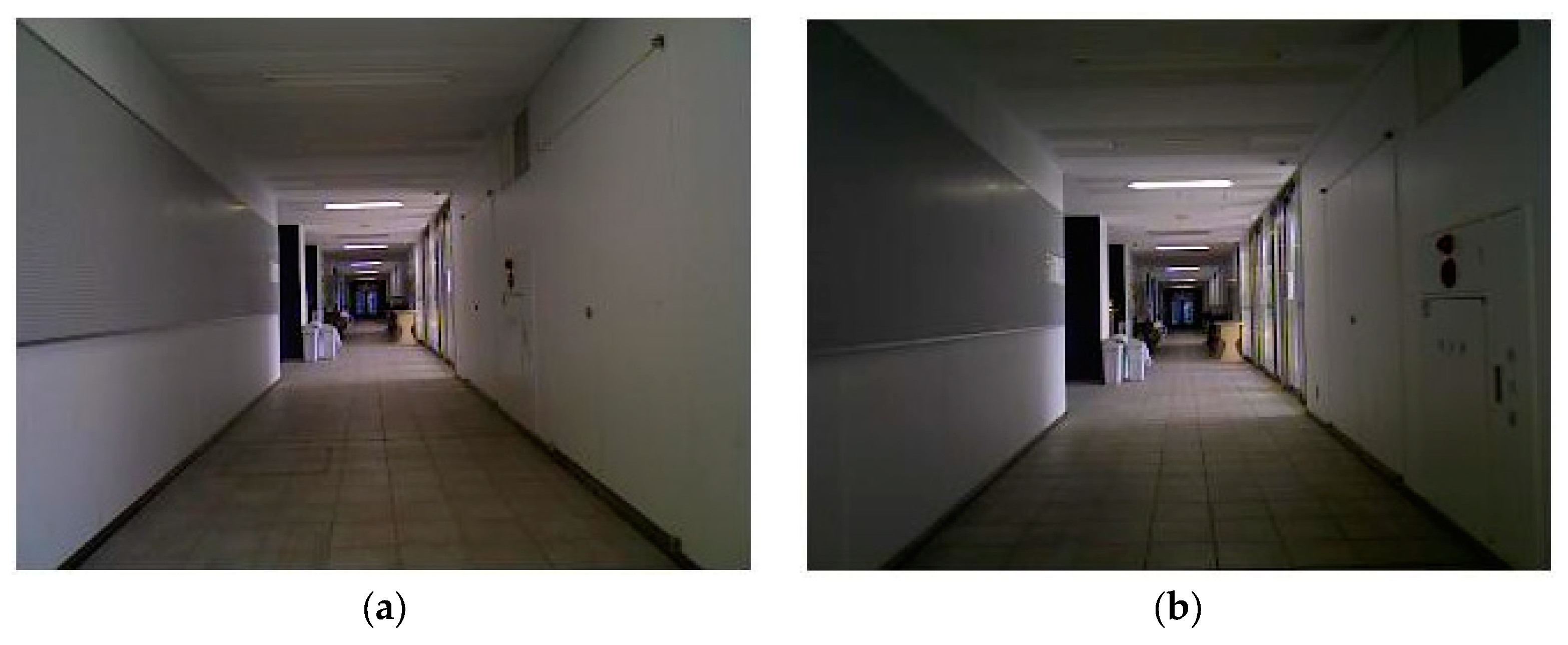
Figure 1 shows the images in two separate positions. The scenes are very similar and both images do not have many features. Therefore, it is difficult to distinguish the two images by using only one type of feature such as SURF, SIFT, or HOG. In the proposed method, we will combine multiple features and depth information to address the problem of localization in textureless environments. The robot location is determined by matching the query image with the precollected geotagged images saved in the dataset. The method performs well in different lighting conditions. With less amount of computation, the localization speed is fast enough which is suitable for real-time robot navigation.
The succeeding sections in this paper are as follows.
Section 2 presents the related works. The methodology is presented in
Section 3. In
Section 4, we present the experimental setup and results. Finally, the conclusion is presented in
Section 5.
2. Related Works
One of the few methods for localization in textureless environments was proposed by Watanabe et al. [
11]. An omnidirectional camera was used to capture the image. The lines extracted from the sequence of at least three images were matched to estimate the camera movement. The performance of this method is based on line detection within an image sequence. The changes in illumination between the images can affect the detection results. Jonghoon Ji et al. [
12] used both vanishing points and door plates as the landmarks for EKF SLAM to increase the stability of the SLAM process in the corridor environment. Khalid Yousif et al. [
13] proposed a 3D SLAM method using Rank Order Statistics (ROS). The authors used ROS to extract 3D key points. However, the common disadvantage of a SLAM-based navigation method is its complexity and high computational requirement. The lighting condition is also a key issue that affects the performance of vision-based SLAM [
14]. Moreover, in large-scale environments such as the long corridor of a big building, it is unnecessary to build a map. Instead, topological navigation can help increase robot speed. In this navigation method, we only have to localize in some positions of the environment. The content-based image retrieval can be applied to search for these positions. There are several methods to retrieve the images in the database. Bhuvana et al. [
15] proposed a method based on SURF features. Bouteldja et al. [
16] used SURF features and a bag of visual words to retrieve the image. However, in textureless environments, it is difficult to distinguish between the two images by using the SURF features only. Hongwen Kang [
17] proposed an algorithm called Re-Search to match the query image with the precaptured images. Based on the matched images, the position can be determined. The author used a standard salient feature detector which is not very effective in textureless environments [
17]. In this work, we use depth features and two feature descriptors—SURF and HOG—to increase the accuracy of image matching.
The Speeded Up Robust Feature (SURF) is a robust feature detector and descriptor that is widely used for object detection. It is first presented by Herbert Bay et al. [
18] in 2006. The method is inspired by Scale-Invariance Feature Transform (SIFT) descriptor, which has a faster speed [
19]. The method to detect and extract feature is similar in the two descriptors. The process of SURF and SIFT has the following steps; Scale-space extrema detection, key point localization, orientation assignment, and key point descriptor. SURF is faster compared with SIFT because there are some improvements in each step. SURF is based on the Hessian matrix to detect the points of interest. However, instead of using difference measure as in Hessian Laplace detector, SURF relies on the determinant of the Hessian to select the location and the scale. SURF uses the wavelet response in vertical and horizontal directions and then assigns the main orientation. All steps use the integral image, resulting in short processing time.
Histogram of Oriented Gradients (HOG) is a feature descriptor that was first introduced by Robert K.McConnell [
20] in 1986. The descriptor is robust for object recognition because it is invariance to the geometric and photometric transformations. To extract the HOG features, the image is divided into cells and then compile the histogram of gradient directions for all the pixels in every cell. The HOG descriptor for the image is the concatenate of all the histograms in all the cells.
HOG feature extraction process consists of three steps: gradient computation, histogram compilation, and histogram concatenation. In the first step, an image is divided into cells of 8 × 8 pixels. The gradient of every pixel relative to the neighbor pixels is computed by applying the filter [−1, 0, 1] for horizontal gradient (x-gradient) and filter [−1, 0, 1]T for vertical gradient (y-gradient). Based on the x-gradient and the y-gradient, the magnitude and angle gradient are calculated. Next step is histogram compilation. A histogram includes a number of bins. In our implementation, we used nine bins. Every bin represents an angle from 0 to 180 degrees (every 20 degrees). The magnitude of a bin is the sum of the gradient magnitude of all the pixels that have the gradient angle close to the bin’s angle. Finally, the histograms of all the cells in the image are concatenated. A block of 2 × 2 cells can be normalized to increase the illumination and shadowing invariance.
3. Methodology
The proposed method is shown in
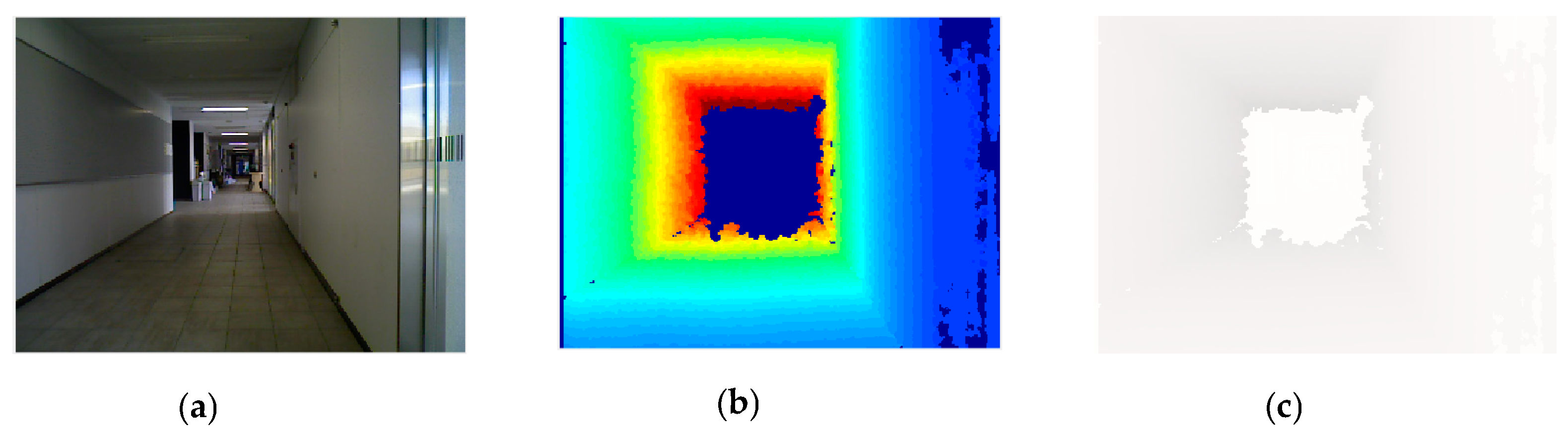
Figure 2. First, we collected a dataset of images in the environment. Every image is tagged with the location where it is taken. Therefore, it is called geotagged image database. In order to increase the image encoding and matching speed, we created only one dataset of D-RGB images instead of separate Depth and RGB image datasets.
Figure 3 shows a sample D-RGB image. It is a combination of Depth image and RGB image to form a 4D image. By extracting the features of all the images in dataset and then applying the K-means clustering on the extracted features we obtain a number of groups of similar features. Each group is called a visual word. All the visual words form a visual vocabulary that is later used to encode the images in the dataset or the query image. In the query step, the encoded query image is compared to all the encoded images in the dataset to find the best-matched image. Based on the geotagged of the best-matched image, the robot location is determined.
3.1. Visual Vocabulary
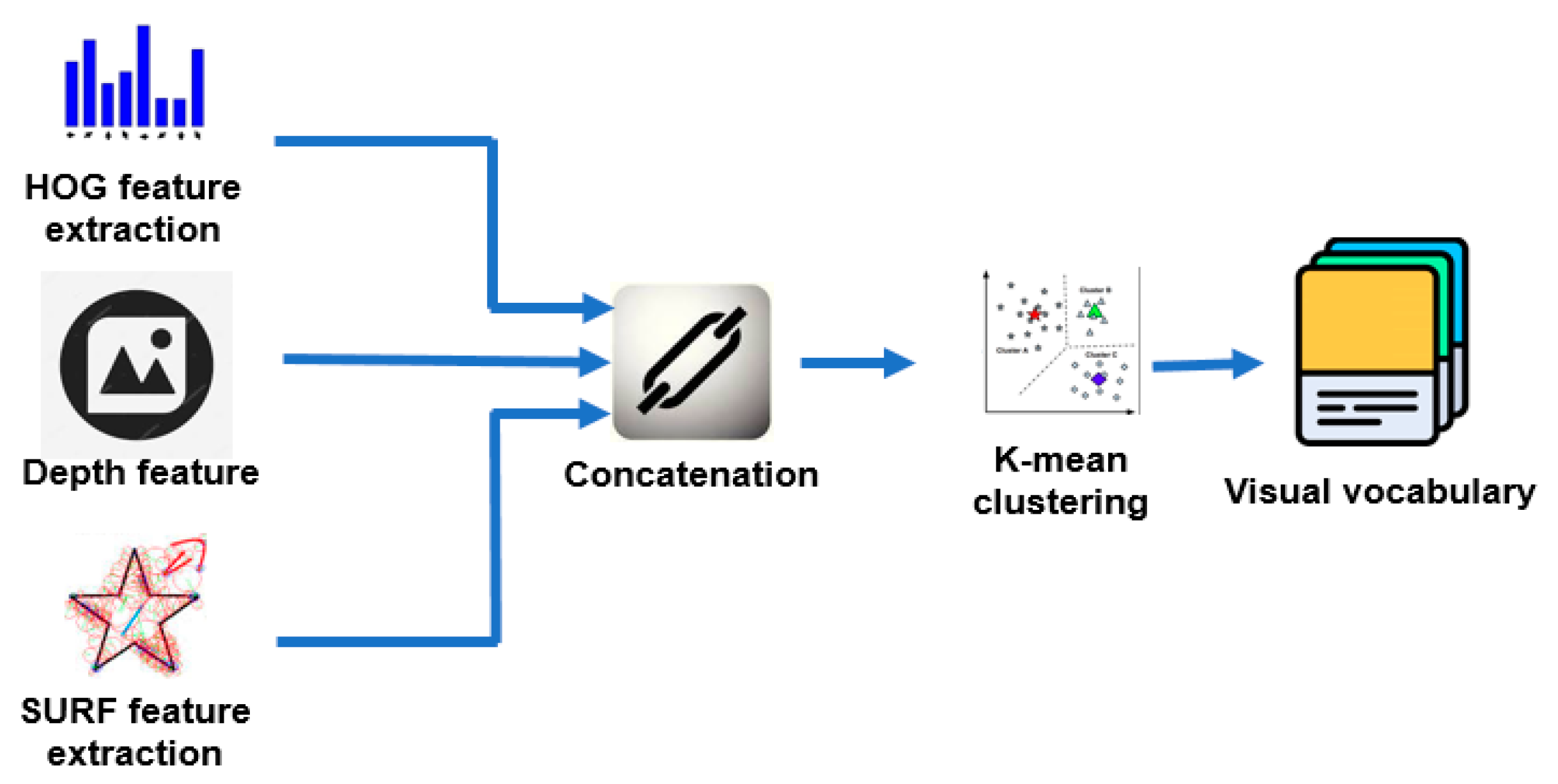
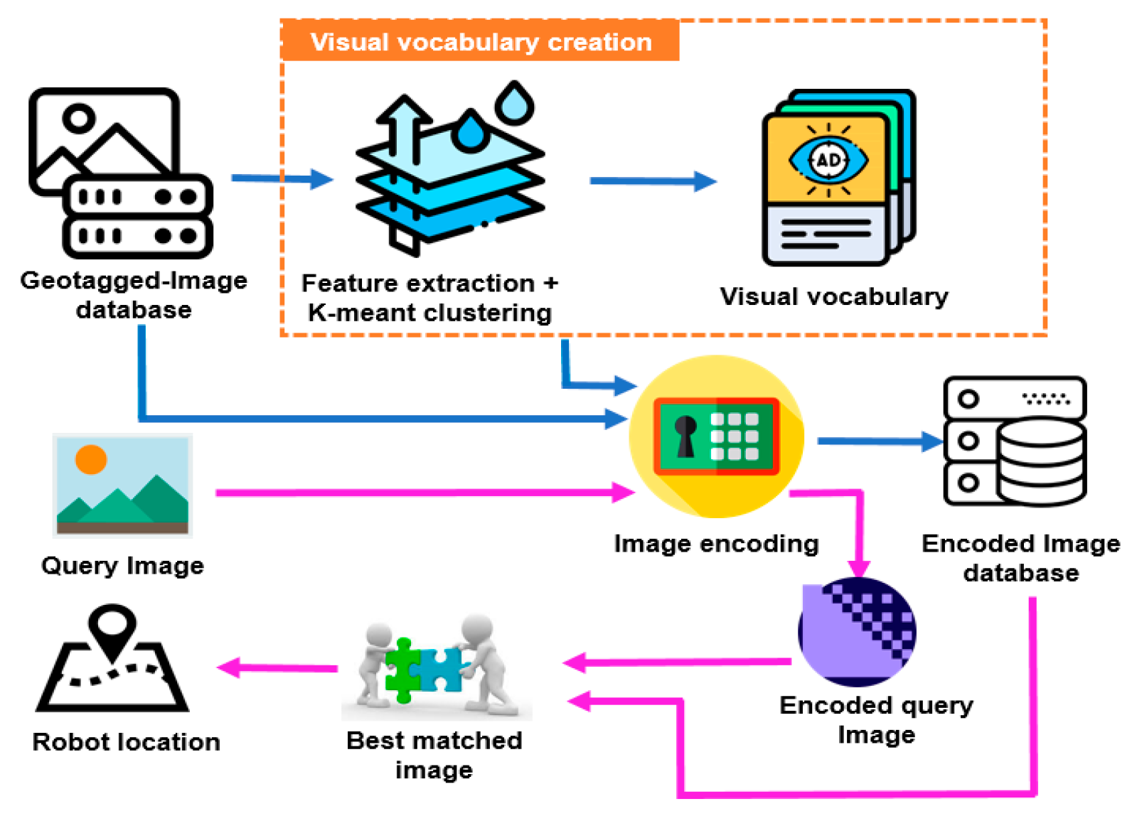
The most important process of the method is the visual vocabulary creation step. This step is demonstrated in detail in
Figure 4. First, we extracted the features of all the images. Three types of features—SURF, HOG, and Depth—are used. HOG and SURF features proved to be effective for object detection [
21,
22,
23]. Depth features supply information about the distance from the robot to surrounding objects. Combination of the three features forms a strong feature for robot localization. We used SURF detector to select the points of interest. After that, the SURF and HOG features at the detected points are extracted. We selected only 80 percent of the strongest extracted features in order to reduce the computation time. The visual vocabulary is created by dividing the obtained features using K-means clustering.
3.1.1. Feature Concatenation
The SURF feature is presented by a 64-bit array, while the HOG feature is presented by 36-bit array. We also extracted the depth information of the four pixels surrounding the detected point. Therefore, a Depth-HOG-SURF feature is presented by a 104-bit array. The number of SURF features, HOG features, and Depth features is the same since they are extracted at the detected SURF points. Therefore, we can concatenate the features horizontally to form a feature matrix that has 104 columns. The number of rows is equal to the number of detected SURF points. Applying the process to all the images in the dataset, we obtain all the Depth-HOG-SURF features.
3.1.2. K-Means Clustering
K-means clustering is a popular method to analyze the data. The input is the data to be divided into clusters and the number of clusters. In our implementation, the data are all the Depth-HOG-SURF features of the images in the dataset. The output is the data divided into clusters. Basically, the clustering process consists of the following steps. First, the center of every cluster is selected randomly. Second, the distance from the centers to all the data points is calculated to determine the nearest cluster center. Assigning the data point to the generated nearest center. Third, the new centers of the clusters are calculated. The process is repeated until the permanent cluster centers are obtained.
After applying the k-means clustering, we have already divided our data into clusters that we called visual vocabulary. The visual vocabulary is used to encode the images in dataset and query images.
3.2. Image Encoding and Image Matching
This step aims to present the images in a form that is easy to search for the best-matched image. So, the processing time decreases, which is very important in robot localization tasks. To encode an image, we extracted the Depth-HOG-SURF features of the image and then compared them with the visual vocabulary to determine the visual words and number of words that appear in the image. After that, we compile the histogram of visual words of that image.
As the robot navigates in the environment, the robot captured image is encoded using the visual vocabulary. Next, we started the comparison with all the histograms in the database to find the best-matched image. Based on the geotag of the best-matched image, the robot’s location is determined.
4. Experimental Setup and Results
This section presents three experimental setups to evaluate the proposed method in different environments and different lighting conditions.
4.1. Experimental Setup
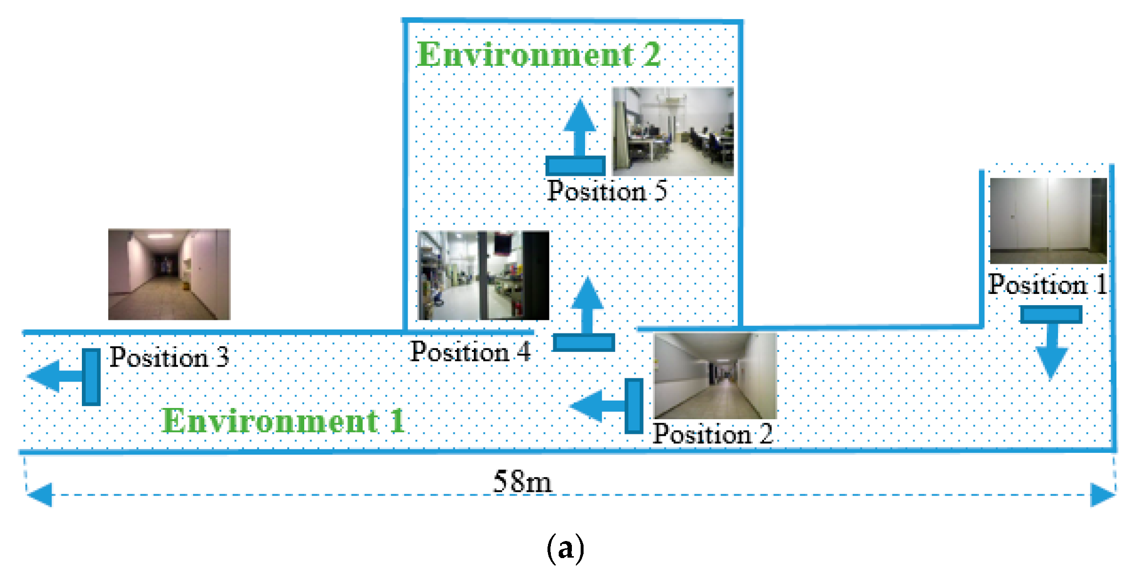
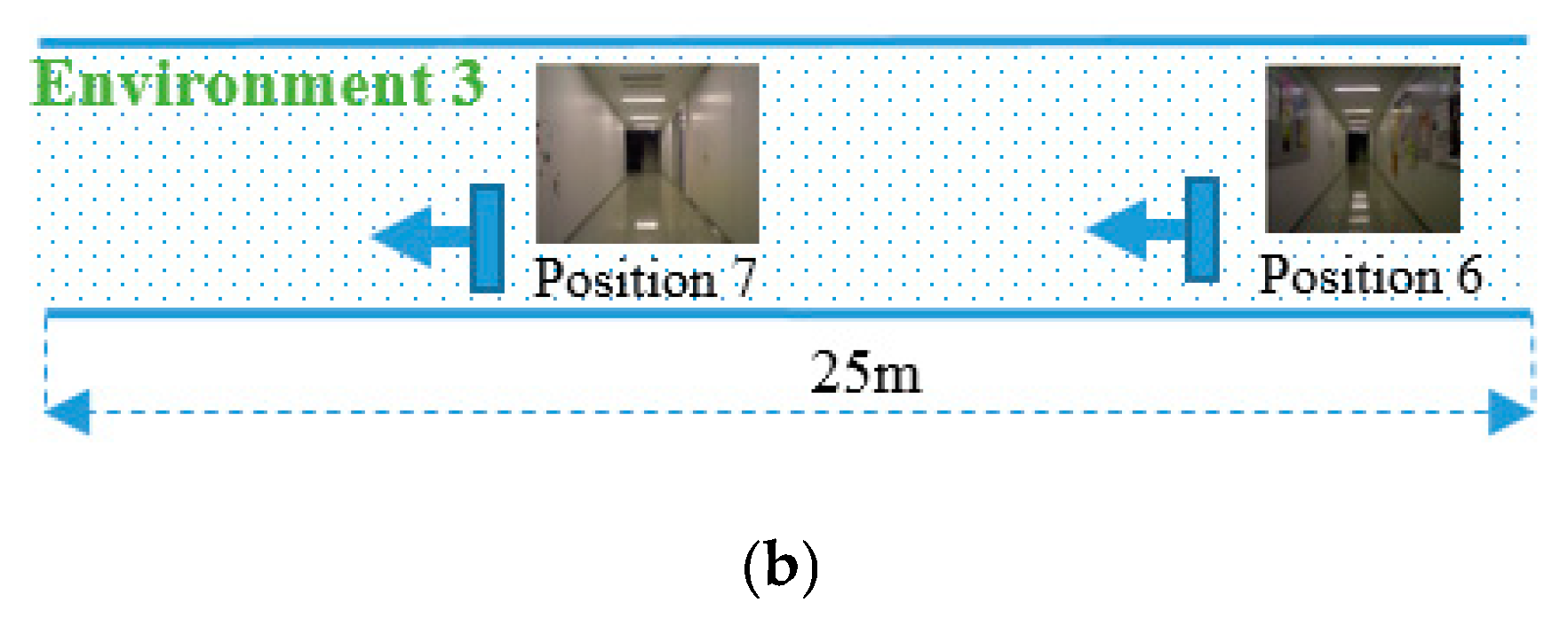
We validated the proposed localization methods in three different environments, as shown in
Figure 5. The first environment is a long corridor with some static objects. The second environment is inside the lab, in which the visual scene is subject to changes every time the third environment is a long corridor without any object; the scenes are almost the same in all positions. In the first environment, the robot localization is done in four positions, in the second environment in one position and in the third environment in two positions. We divided the experiments into three parts: (1) experiments with the precaptured images in the test set; (2) experiments for robot localization; and (3) topological robot navigation based on the proposed method. All the experiments are done using MATLAB R2018a installed in the Intel (R) Core (TM) i5-6200U CPU 2.30 GHz laptop. In order to show the effectiveness of the proposed method, we compare the results with HOG feature matching, ORB feature matching, and SURF feature image indexing methods.
The image dataset for training contains 1400 images of all seven locations. This test dataset also contains 1400 images to validate the success rate. The images are taken in different lighting conditions. By extracting all the features of the image dataset we obtained 14,000,000 Depth-HOG-SURF features. Clustering the extracted features into 1000 groups corresponds to 1000 visual words in the vocabulary. We tried with a different number of visual words but 1000 words gave the best localization results.
Table 1 gives the comparison of the localization results with different number of visual words. In this experiment, we captured 500 images at four positions. There are three possible results: correct localization, wrong localization, and cannot localize. The correct and wrong localization are used in the case when the robot real location and generated topological localization are the same or different, respectively. For example, if the robot is in position 1 and the algorithm generates geotag position 1, the result is “correct localization”, otherwise it is “wrong localization”. “Cannot localize” is when the robot cannot find the matched image in the database; therefore its position cannot be determined.
When the number of visual words is small, the best-matched image is easy to generate. However, the matched image does not correspond to the image of the correct robot location. Therefore, the number of wrong localization images is high (10 images). In contrast, when the number of visual words is high, it is difficult to find the best-matched image. Sometimes, the robot captured an image at one of the four positions but cannot find the matched image in the database, resulting in a large number of “cannot localize” answers (seven images).
4.2. Results
This section discusses the experimental results of the proposed method: evaluating the success rate using the images in the test set, robot localization, and topological robot navigation.
4.2.1. Experiments with the Images in the Test Set
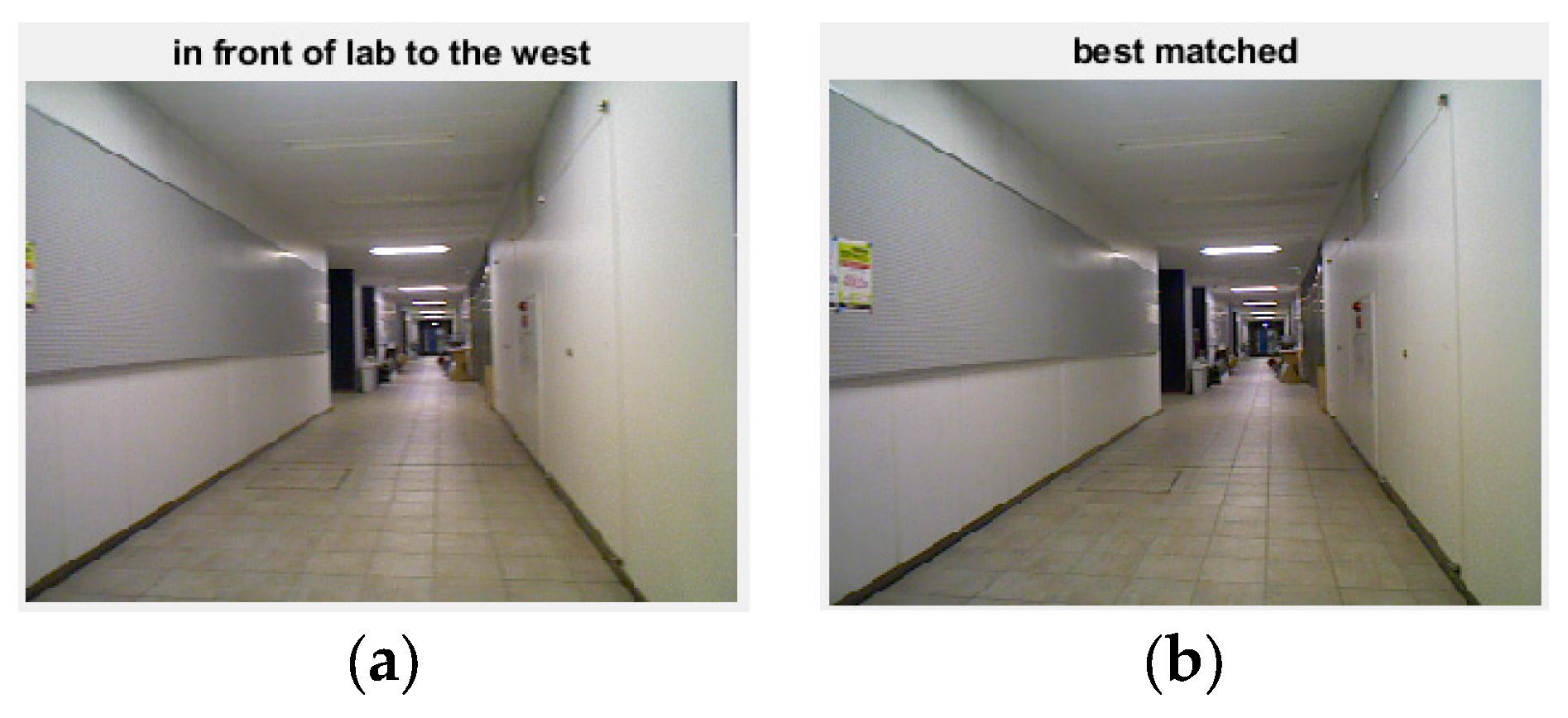
Figure 6 shows the captured and the best-matched image.
Figure 6a is the query image in the test set and
Figure 6b is the best-matched image taken from image dataset. The geotagged of the best-matched image is “in front of lab to the west”, so that the robot is localized at this position. Among the 1400 images in the test set, the number of correct best-matched images was 1375 images. Therefore the success rate is 98.21%.
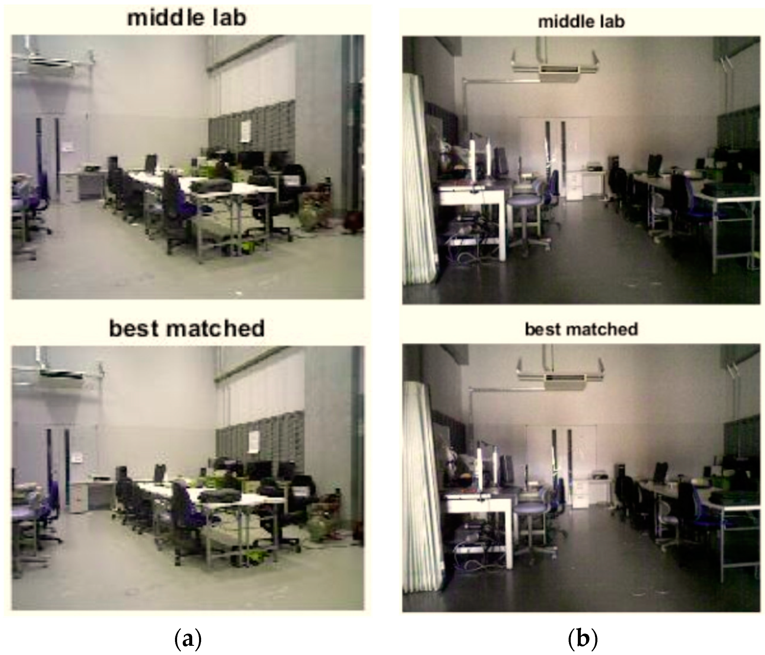
In order to further verify the performance of the proposed method, the experiments were also performed in different lighting conditions (
Figure 7).
Figure 7a shows the result in the good lighting condition.
Figure 7b shows the result at the same position, but in the insufficient lighting condition. In both environmental conditions, the robot can localize exactly its position as “middle lab”.
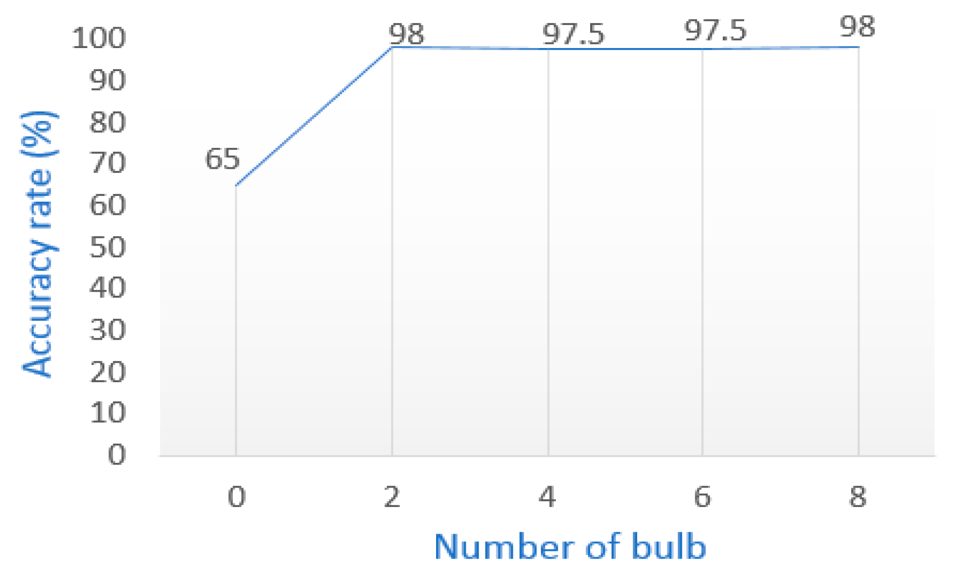
Figure 8 shows the localization accuracy at the position “middle lab” when the lighting condition is gradually reduced.
Table 2 shows the detail localization results for seven positions. Positions 1 to 4 are in environment 1, position 5 is in environment 2, and positions 6 and 7 are in environment 3.
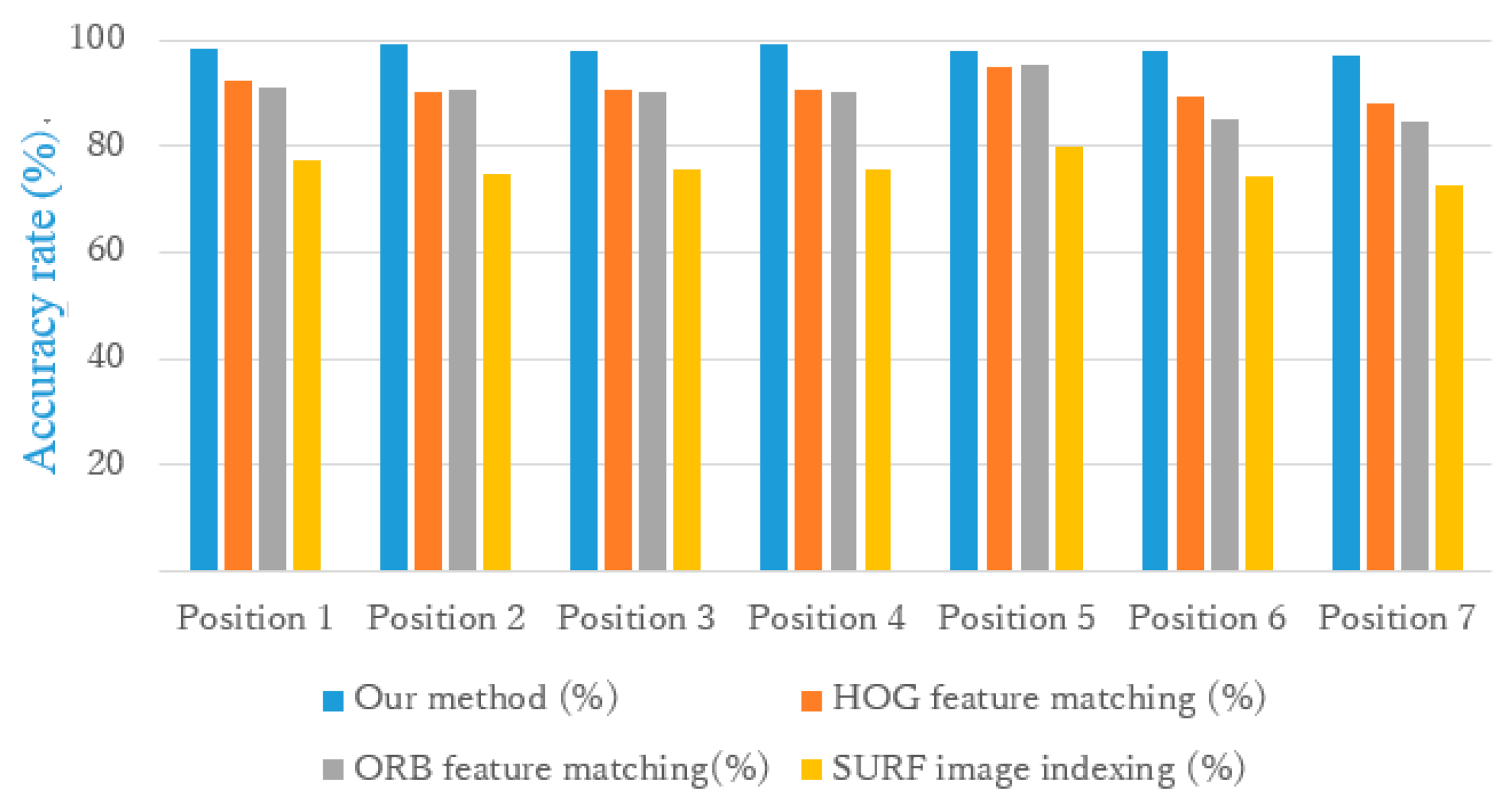
Figure 9 shows the comparison results with the HOG feature matching, ORB feature matching, and SURF feature image indexing methods. In all the seven locations, our method gave a better localization success rate. Especially in environment 3 (positions 6 and 7), where there is almost no feature, our method performed better than three other methods. In environment 2 (position 5), because there are more features, the HOG and ORB feature matching methods resulted in the same performance as our method.
4.2.2. Experiments for Robot Localization
We also conducted experiments for robot localization. For the robot running in the environment we captured 1011 images. The number of images correct matches is 996. Therefore, the success rate is 98.51%.
Table 3 is a comparison with other methods. The experimental results show that our method performed better than others. The SURF feature image indexing method has a shorter computation time but gave poor localization results. Our method is fast enough to apply for real time robot localization and navigation.
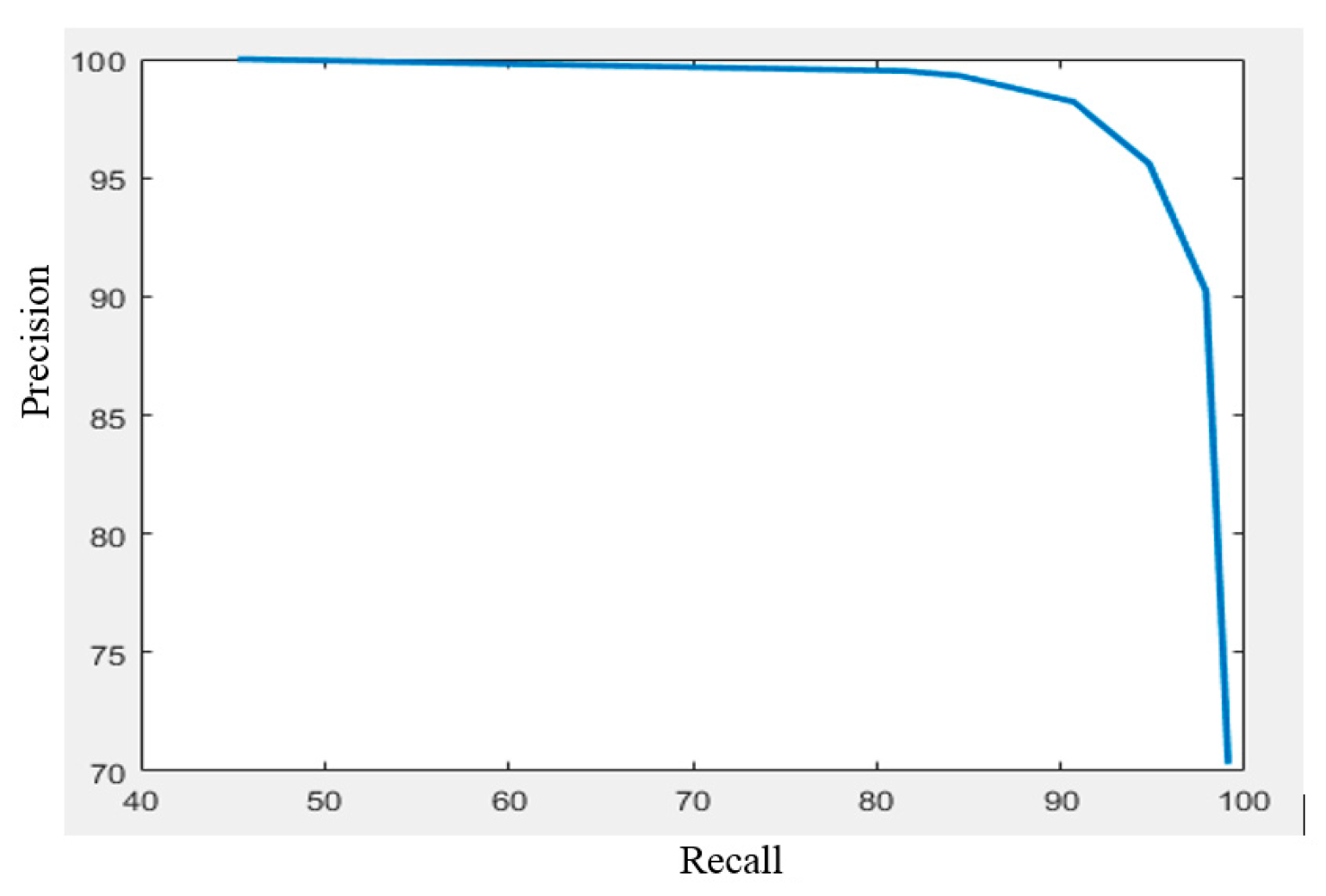
Figure 10 is the precision–recall curve of the proposed method. To generate the curve, we change the threshold of the image matching process. When the threshold is increased, it is difficult to match the query image with the images in the database. Therefore, the recall decreases and the precession increases.
4.2.3. Topological Navigation
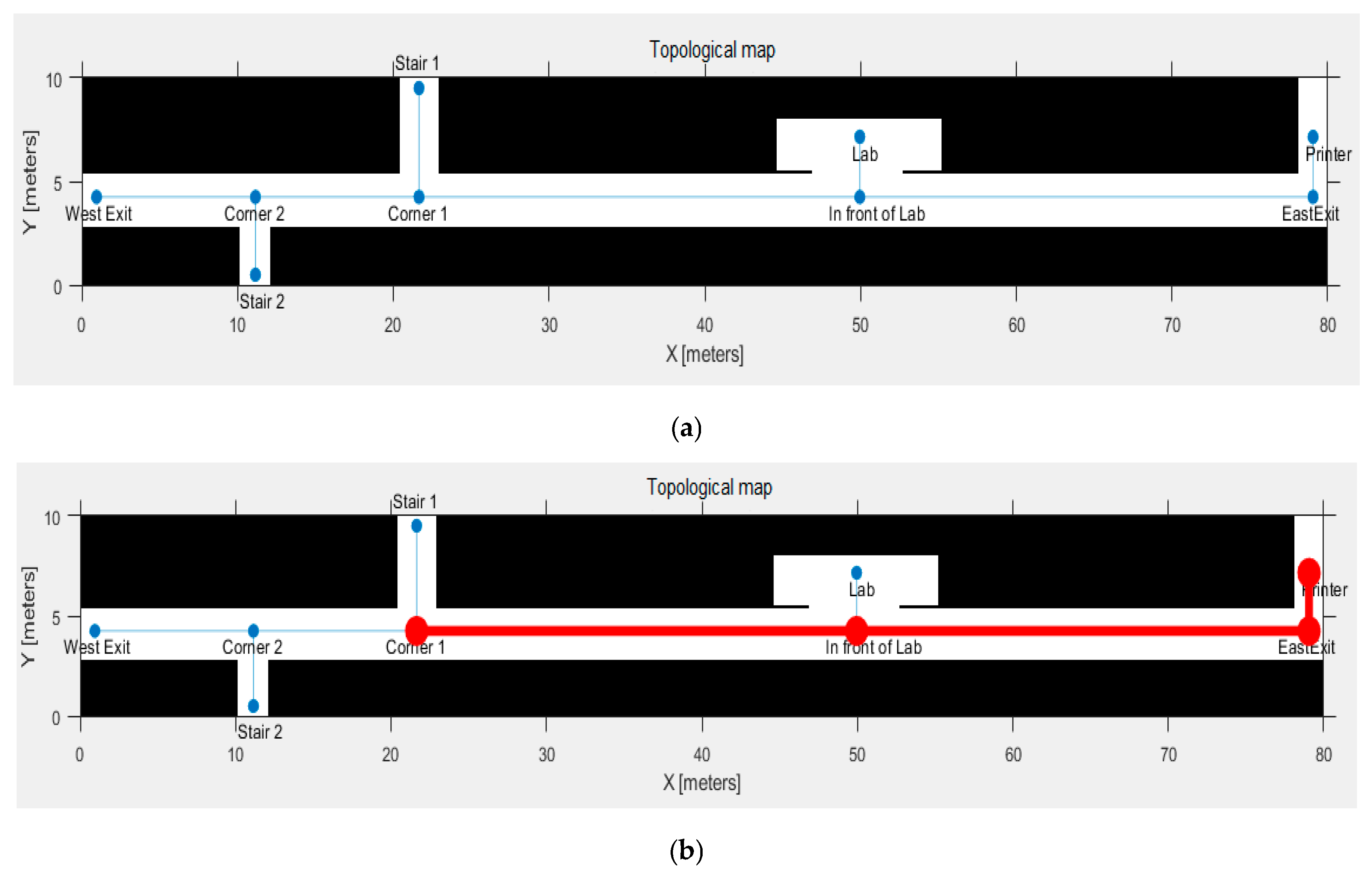
In this experiment, we apply the proposed localization method for robot navigation in a topological map, as shown in
Figure 11a. The environment is the corridor on the first floor of the north building, Hosei University, Koganei Campus; it is 80 meters long. The robot will move from the initial position “Printer” to the target position “Corner 1”. The path is “Printer”, ‘’East Exit”, “In front of Lab”, “Corner 1”. The navigation result is shown in
Figure 11b. The robot successfully localized and passed all the middle nodes to get to the target.


