MIMO PID Controller Tuning Method for Quadrotor Based on LQR/LQG Theory

Abstract

In this work, a new pre-tuning multivariable PID (Proportional Integral Derivative) controllers method for quadrotors is put forward. A procedure based on LQR/LQG (Linear Quadratic Regulator/Gaussian) theory is proposed for attitude and altitude control, which suposes a considerable simplification of the design problem due to only one pretuning parameter being used. With the aim to analyze the performance and robustness of the proposed method, a non-linear mathematical model of the DJI-F450 quadrotor is employed, where rotors dynamics, together with sensors drift/bias properties and noise characteristics of low-cost commercial sensors typically used in this type of applications are considered. In order to estimate the state vector and compensate bias/drift effects in the measures, a combination of filtering and data fusion algorithms (Kalman filter and Madgwick algorithm for attitude estimation) are proposed and implemented. Performance and robustness analysis of the control system is carried out by employing numerical simulations, which take into account the presence of uncertainty in the plant model and external disturbances. The obtained results show the proposed controller design method for multivariable PID controller is robust with respect to: (a) parametric uncertainty in the plant model, (b) disturbances acting at the plant input, (c) sensors measurement and estimation errors.

1. Introduction

Small unmanned aerial vehicles (SUAV) are used in a great variety of application fields [1,2,3]. In order to achieve the required level of performance, the vehicle must include a proper automatic control system as well as electronics, sensors, communications, and signal processing algorithms. To develop and validate the control system is very useful to count with an accurate mathematical model of the vehicle, sensors and actuators dynamics [4,5,6,7,8,9,10,11,12,13]. The present work uses the model structure exposed in [6,12,14] as a starting point but, as a novel contribution, introduces a nonlinear mathematic model (obtained experimentally) of the rotors used in the DJI F-450 quadrotor (Figure 1), that is used to perform a more detailed and realistic analysis of the control system through numerical simulations.

One crucial concern to allow the indoor operation of a SUAV is the attitude and position estimation, typically based on the use of inertial measurement units (IMU) type MEMS (MicroElectroMechanical Systems) and cameras [6,8,15,16,17,18,19,20,21]. To estimate the attitude, position and velocity state variables of the vehicle from the measurements provided by the sensors, a variety of methods are used, such as Kalman filters (KF) [6,16,22,23], extended Kalman filters (EKF) [21,22,23,24] and complementary filters [4,25] among others.

Several methods have been published to control the fly of SUAV [1,2,5,9,10,11,13,17,26,27,28,29,30,31,32,33,34,35,36,37,38,39], of which [17,30,31,33,35,36,37,38,39] use PID (Proportional Integral Derivative) controllers for attitude, altitude and/or horizontal position. However, as MIMO (Multiple-input Multiple-output) systems, the tuning of PID controllers for multi-rotor vehicles is not an easy issue. On the other hand, authors such as [5,29,30,31,32,33,34,35] use LQR/LQG (Linear Quadratic Regulator/Gaussian) control, since it allows the design of the control system considering the whole coupling of the vehicle. Even so, a deep knowledge of the system is required to tune the weighting matrices [40]. Furthermore, in practice, in order to achieve a controller faster than the classic LQR structure and robust to the errors present in the estimated state vector, some authors [31,35] use a nested control loop that combines PID and LQR controllers, which complicates the design issue. In this context, we propose a new and practical pre-tuning method based on the LQR/LQG theory for PID controllers applied to the altitude and attitude control of multirotor systems, in particular, a quadrotor. The main contribution of this work, with respect to the above techniques, is that this method of pre-tuning obtains the twelve gains of a standard control structure widely used in multirotor systems (four PID controllers: three for the attitude and one for the altitude) through the design of a MIMO LQR/LQG controller using only one pre-tuning parameter, which considerably simplifies the design problem. Therefore, our work is focused on the oriented toward applications, and specifically in the practical issue to develop a systematic method for a multivariable PID controller tuning.

Additionally, the uncertainty affecting the measurements are taken into account through the errors and noise modelling of a LIDAR, an optical flow camera, and a MEMS type MARG (Magnetic, Angular Rate, Gravity) sensor [42,43,44,45]. The attitude of the vehicle is estimated using the sensor fusion algorithm proposed in [46], whereas the altitude and the vertical velocity are estimated by means of a Kalman filter. Thus, this study considers the effects of measurement errors, including the relatively large bias and noise errors inherent to the MEMS sensors technology, and includes all the required estimation and compensation algorithms necessary for implementation in a real system. A horizontal controller is also included to analyze the influence of an external control loop over the proposed modified LQR/LQG. Next, we study the performance and the robustness of the proposed controller design method through numeric simulations, considering a non-linear model of the DJI F-450 quadrotor and the rotors non-linear dynamics obtained experimentally. The influence of uncertainty and bounded perturbations on the robustness of the control system is also tested adding parametric uncertainty and significant external disturbances.

The organization of this paper is as follows: In Section 2, the mathematical model obtained experimentally, which is used to the analysis and evaluation of the control system, is presented, followed by a simplified model used for controller design. In Section 3, the proposed design methodology to obtain the attitude and altitude control laws, as well as the employed state estimation algorithms, are described. In Section 4 address the problem of the estimation and control of the horizontal position. Section 5 provides numeric simulation results. Finally, conclusions are drawn in Section 6.

2. Mathematical Model

To carry out the synthesis and evaluation of the control system two different models of the DJI F-450 quadrotor will be developed. The first is a non-linear model to analyze and evaluate (AEM model) the designed controllers. This model incorporates the effects of the rotors dynamics and measurement errors. The second is a non-linear model for control system design (CDM model). This model includes some simplifications compared with the previous one that will lead to a linear model. The linear model is used to design the controllers and in several estimation algorithms.

2.1. Analysis and Evaluation Model (AEM)

As it was said previously, the present work uses the model structure exposed in [6,12,14] as a starting point. Figure 2 shows the Earth and Body reference frames. The translation dynamics equations are:

$$\begin{array}{cc}\hfill m\dot{u}& =(cos\varphi sin\theta cos\psi +sin\varphi sin\psi )T_b-K_{dx}u\left|u\right|\hfill \\ \hfill m\dot{v}& =(cos\varphi sin\theta sin\psi -sin\varphi cos\psi )T_b-K_{dy}v\left|v\right|\hfill \\ \hfill m\dot{w}& =(cos\varphi cos\theta )T_b-K_{dz}w\left|w\right|-mg\hfill \\ \hfill T_b& =T_1+T_2+T_3+T_4\hfill \end{array}$$

(1)

where $(x_E,y_E,z_E)$ is the position vector of the vehicle relative to the Earth frame, $(u,v,w)$ is the linear velocity ($u={\dot{x}}_E$, $v={\dot{y}}_E$, $w={\dot{z}}_E$), and $T_b$ is the total thrust force generated by the four rotors relative to the Body reference frame. On the other hand, the rotational dynamics is described by:

$$\begin{array}{c}{I}_{xx}\dot{p}=(T_2-T_4)l-qr(I_{zz}-I_{yy})\hfill \\ I_{yy}\dot{q}=(-T_1+T_3)l-pr(I_{xx}-I_{zz})\hfill \\ I_{zz}\dot{r}=\left(-N_1^2+N_2^2-N_3^2+N_4^2\right)K_P-(I_{yy}-I_{xx})qp\hfill \\ \dot{\varphi }=p+qsin\left(\varphi \right)tan\left(\theta \right)+rcos\left(\varphi \right)tan\left(\theta \right)\hfill \\ \dot{\theta }=qcos\left(\varphi \right)-rsin\left(\varphi \right)\hfill \\ \dot{\psi }=qsin\left(\varphi \right)sec\left(\theta \right)+rcos\left(\varphi \right)sec\left(\theta \right)\hfill \end{array}$$

(2)

where $(\varphi ,\theta ,\psi )$ represents the attitude using Euler angles, $(p,q,r)$ is the angular velocity vector (measured in the Body frame), $T_i$ is the thrust force generated by the i rotor (relative to the Body frame), and $N_i$ is the rotation frequency of the i rotor (in RPM), for $i\in \{1,2,3,4\}$.

Table 1. Model parameters of the DJI F-450 quadrotor used for analysis and evaluation.

Simbol	Description	Value
$K_{dx}$	Aerodynamic drag coefficient using a reference area perpendicular to x axis	0.01212 Kg/m
$K_{dy}$	Aerodynamic drag coefficient using a reference area perpendicular to y axis	0.01212 Kg/m
$K_{dz}$	Aerodynamic drag coefficient using a reference area perpendicular to z axis	0.0648 Kg/m
$K_{T1}$	Thrust—RPM quadratic relation	$1.0155\times {10}^{-7}$ N/RPM2
$K_{T2}$	Thrust—RPM gain	$-1.0327\times {10}^{-4}$ N/RPM
$K_P$	Torque—RPM quadratic relation	$3.46\times {10}^{-8}$ N m/RPM2
$K_f$	Thrust—Duty cycle gain	0.0667 N/%
l	Distance from the center of one motor to the center of gravity of the system	0.235 m
m	System mass	1.250 Kg
$I_{xx}$	Moment of inertia about x axis	0.0094 Kg m2
$I_{yy}$	Moment of inertia about y axis	0.01 Kg m2
$I_{zz}$	Moment of inertia about z axis	0.0187 Kg m2
g	Gravitational acceleration	9.81 m/s2

shows the parameters values of the model (1) and (2), that have been obtained experimentally [47] through laboratory tests with the DJI F-450 quadrotor used in this work.

The inputs of the subsystem composed by the electronic speed controllers (ESC), the brushless motors, and the propellers are the duty-cycles values of the PWM (Pulse Width Modulation) signal applied to each ESC, $D_i$, and its outputs are the thrust forces and torques developed by each rotor. Despite the model structure being based on that proposed by [6,12,14], its parameters have been identified to obtain a trustworthy model of these parts of the DJI F-450 quadrotor. The identification has been carried out applying step and ramp signals to the inputs ($D_i$) and recording the rotation frequencies, thrusts, and torques. The following equipment has been used to accomplish the tests: a calibrated SEN-CC-FZ1439 load cell, a QDR1114 optical sensor functioning as a tachometer, an NI USB-6211 acquisition system, and an LPC4088-32 microcontroller development board. Figure 3 shows one of the experimental set-ups. The reference [47] provides further details.

Each group ESC-motor-propeller is modeled as a first-order system with delay, whose dynamics are described by

$$\tau \dot{N}\left(t\right)+N\left(t\right)=KD(t-{\tau }_d)$$

(3)

where $\tau$ is the system time constant, ${\tau }_d$ is the delay, and K is the stationary gain. The values derived experimentally in the hover equilibrium condition were: $\tau =0.038$ s, ${\tau }_d=0.012$ s y $K=82.3$ $RPM/\%$.

The experimental relations that link the rotational frequency N (in RPM) with the thrust, T, and the torque, P, developed by each rotor are given by the Equations (4) and (5), respectively.

$$T=K_{T1}{N}^2+K_{T2}N$$

(4)

$$P=K_P{N}^2$$

(5)

In order to carry out a realistic analysis and design, the errors and noise levels of conventional commercial sensors employed in these type of systems have been obtained from the manufacturer manuals and introduced in the model. These sensors are a PulsedLight LIDAR-LITE laser range sensor [42], an InvenSense MPU-9250 MARG [43,44], comprising a 3-Axis gyroscope, a 3-Axis accelerometer, and a 3-Axis magnetometer, and a PX4-FLOW optical flow camera [45].

2.2. Control System Design Model (CDM)

To ease the task of designing the controller, we will build a simplified model relative to the one presented in the previous section. The main differences between the two are the following:

• The CDM model does not take into account the rotor dynamics.
• The thrust and the torque are linear functions of the PWM signals duty-cycle.
• The rotational dynamical model assumes relative low angular velocities and small enough Euler angles.

After applying the cited simplifications, the CDM model is defined by the system of non-linear Equations (6). Table 1 shows the parameter values of this model.

$$\begin{array}{cc}\hfill p& =\dot{\varphi },q=\dot{\theta },r=\dot{\psi }\hfill \\ \hfill I_{xx}\dot{p}& =U_{\varphi }-qr(I_{zz}-I_{yy})\hfill \\ \hfill I_{yy}\dot{q}& =U_{\theta }-pr(I_{xx}-I_{zz})\hfill \\ \hfill I_{zz}\dot{r}& =U_{\psi }-qp(I_{yy}-I_{xx})\hfill \\ \hfill u& ={\dot{x}}_E,v={\dot{y}}_E,w={\dot{z}}_E\hfill \\ \hfill m\dot{u}& =(cos\varphi sin\theta cos\psi +sin\varphi sin\psi )U_z-K_{dx}u\left|u\right|\hfill \\ \hfill m\dot{v}& =(cos\varphi sin\theta sin\psi -sin\varphi cos\psi )U_z-K_{dy}v\left|v\right|\hfill \\ \hfill m\dot{w}& =(cos\varphi cos\theta )U_z-K_{dz}w\left|w\right|-mg\hfill \end{array}$$

(6)

The relations between the components of the $\mathbf{U}$ and $\mathbf{D}$ vectors (the duty-cycles of the four PWM signals) is defined by [6]:

$$\underset{\mathbf{U}}{\underbrace{\left(\begin{array}{c}{U}_{\varphi }\\ U_{\theta }\\ U_{\psi }\\ U_z\end{array}\right)}}=\underset{M}{\underbrace{\left(\begin{array}{cccc}0& K_{f}l& 0& -K_{f}l\\ -K_{f}l& 0& K_{f}l& 0\\ -K_P& K_P& -K_P& K_P\\ K_f& K_f& K_f& K_f\end{array}\right)}}\underset{\mathbf{D}}{\underbrace{\left(\begin{array}{c}{D}_1\\ D_2\\ D_3\\ D_4\end{array}\right)}}$$

(7)

where $\mathbf{D}$ is the vector of duty-cycles, and the components of $\mathbf{U}$ are the fictitious control signals $U_{\varphi }$, $U_{\theta }$, $U_{\psi }$ y $U_z$ that allows split control of the attitude ($\varphi$, $\theta$, $\psi$) and the altitude (z) variables. Thus, we can choose between considering the whole 4 × 4 MIMO problem or one 3 × 3 MIMO attitude problem plus one SISO altitude problem instead. The next section elaborates on the first option.

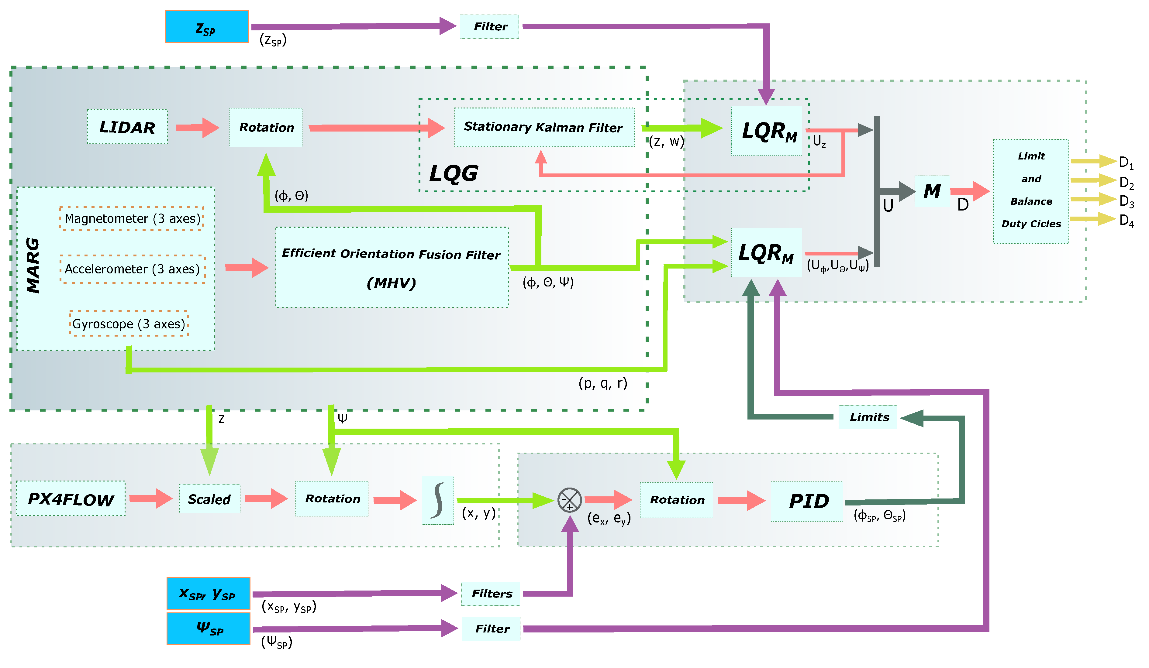
3. Attitude and Altitude Control System

The main objective of this system is the stabilization (hovering) of the vehicle at a certain altitude. Hovering is a manoeuvre in which the quadrotor is maintained in nearly motionless flight over a reference point at a constant altitude and on a constant heading. In order to control the vehicle, the complexity of the system and the strong coupling that exists between the manipulated variables and the controlled variables have been taken into account. Therefore, a multivariable control approach based on state space has been considered [40,48,49]. As a novel contribution of this work for multivariable PID tuning, it is proposed to use a modified LQR/LQG control law, in which feedback is performed considering the tracking error between the state vector and a setpoint or reference state vector. ISpecifically, for the design of the attitude and altitude controller the following state vector, $\mathbf{X}$, is considered:

$${\mathbf{X}}^T=\left(\begin{array}{cccccccc}\varphi & \theta & \psi & z_E& p& q& r& w\end{array}\right)$$

(8)

The manipulated variables (MV) vector, $\mathbf{U}$, is composed of the four components $U_{\varphi }$, $U_{\theta }$, $U_{\psi }$, and $U_z$ given in (6). The process variables (PV) vector, or controlled variables (CV) vector, is given by,

$${\mathbf{Y}}^T=\left(\begin{array}{cccc}\varphi & \theta & \psi & z_E\end{array}\right)$$

(9)

An equilibrium condition for hovering at an altitude $z_{eq}$ is characterized by,

$${\mathbf{X}}_{eq}^T=\left(\begin{array}{cccccccc}0& 0& 0& z_{eq}& 0& 0& 0& 0\end{array}\right),{\mathbf{U}}_{eq}^T=\left(\begin{array}{cccc}0& 0& 0& U_{z_{eq}}\end{array}\right),{\mathbf{Y}}_{eq}^T=\left(\begin{array}{cccc}0& 0& 0& z_{eq}\end{array}\right)$$

(10)

Linearizing the eight non-linear differential equations of the quadrotor model (6) for hover condition, (${\mathbf{X}}_{eq}$, ${\mathbf{U}}_{eq}$, ${\mathbf{Y}}_{eq}$), and considering incremental (or deviation) variables with respect to equilibrium point,

$$x=X-X_{eq},u=U-U_{eq},y=Y-Y_{eq}$$

(11)

the linearized system dynamics is defined by (12).

$$\begin{array}{cc}\hfill \dot{\mathbf{x}}& =A\mathbf{x}+B\mathbf{u}\hfill \\ \hfill \mathbf{y}& =C\mathbf{x}\hfill \end{array}$$

(12)

In order to add integral action to the controller, the system model is modified including four new state variables corresponding to the integral of the tracking error of the controlled variables, resulting in the following augmented state vector,

$${\mathbf{x}}_A=\begin{array}{c}\left(\begin{array}{c}\mathbf{x}\\ {\mathbf{x}}_I\end{array}\right)\end{array}$$

(13)

where ${\dot{\mathbf{x}}}_I=\mathbf{r}-\mathbf{y}$, and $\mathbf{r}$ is the incremental value of the set-point vector, $\mathbf{r}={\mathbf{Y}}_{SP}-{\mathbf{Y}}_{SPeq}$. Therefore, the augmented system matrices are given by,

$$A_a=\left(\begin{array}{cc}A& 0\\ -C& 0\end{array}\right),B_a=\left(\begin{array}{c}B\\ 0\end{array}\right),C_a=\left(\begin{array}{cc}C& 0\end{array}\right)$$

(14)

The conventional LQR control law with integral action (incremental vector value) is given by,

$$\mathbf{u}=-K_c\mathbf{x}+K_I{\mathbf{x}}_I$$

(15)

and the controller output (CO) vector ($\mathbf{U}$) is obtained by,

$$\mathbf{U}={\mathbf{U}}_{eq}+\mathbf{u}$$

(16)

For that, the feedback gain matrices, $K_c$ and $K_I$, must be calculated solving the corresponding algebraic Riccati equation (AREc) [40,48,49], which results from the optimization problem of minimizing a cost function given by,

$$J={\int }_0^{\infty }\left({\mathbf{x}}^T{Q}_c\mathbf{x}+{\mathbf{u}}^T{R}_c\mathbf{u}\right)dt$$

(17)

where $Q_c$ and $R_c$ are the named weighting matrices.

With the LQR controller, the linearized closed-loop control system dynamics (which is an approximation of the nonlinear system for a neighborhood of the equilibrium point defined by the hover condition) is given by,

$$\left(\begin{array}{c}\dot{\mathbf{x}}\\ {\dot{\mathbf{x}}}_I\end{array}\right)=\underset{A_{yr}}{\underbrace{(A_a-B_a{K}_{ca})}}\left(\begin{array}{c}\mathbf{x}\\ {\mathbf{x}}_I\end{array}\right)+B_{yr}\mathbf{r},K_{ca}=(K_c-K_I)$$

(18)

A proposal made in this work is to modify the conventional LQR structure given in (15), where the new control law is defined by,

$$\mathbf{u}=K_c({\mathbf{x}}_{SP}-\mathbf{x})+K_I{\mathbf{x}}_I$$

(19)

where ${\mathbf{x}}_{SP}$ represents the incremental reference (or set-point) state vector to follow,

$${\mathbf{x}}_{SP}^T=\left(\begin{array}{cccccccc}{\varphi }_{SP}& {\theta }_{SP}& {\psi }_{SP}& z_{SP}& p_{SP}& q_{SP}& r_{SP}& w_{SP}\end{array}\right)$$

(20)

The proposed control law (19) gets the same poles for the closed-loop linearized system obtained with (15), but achieves to reduce the time response of the system to set-point changes due to (19) modifies the zeros of the closed-loop system reached with (15).

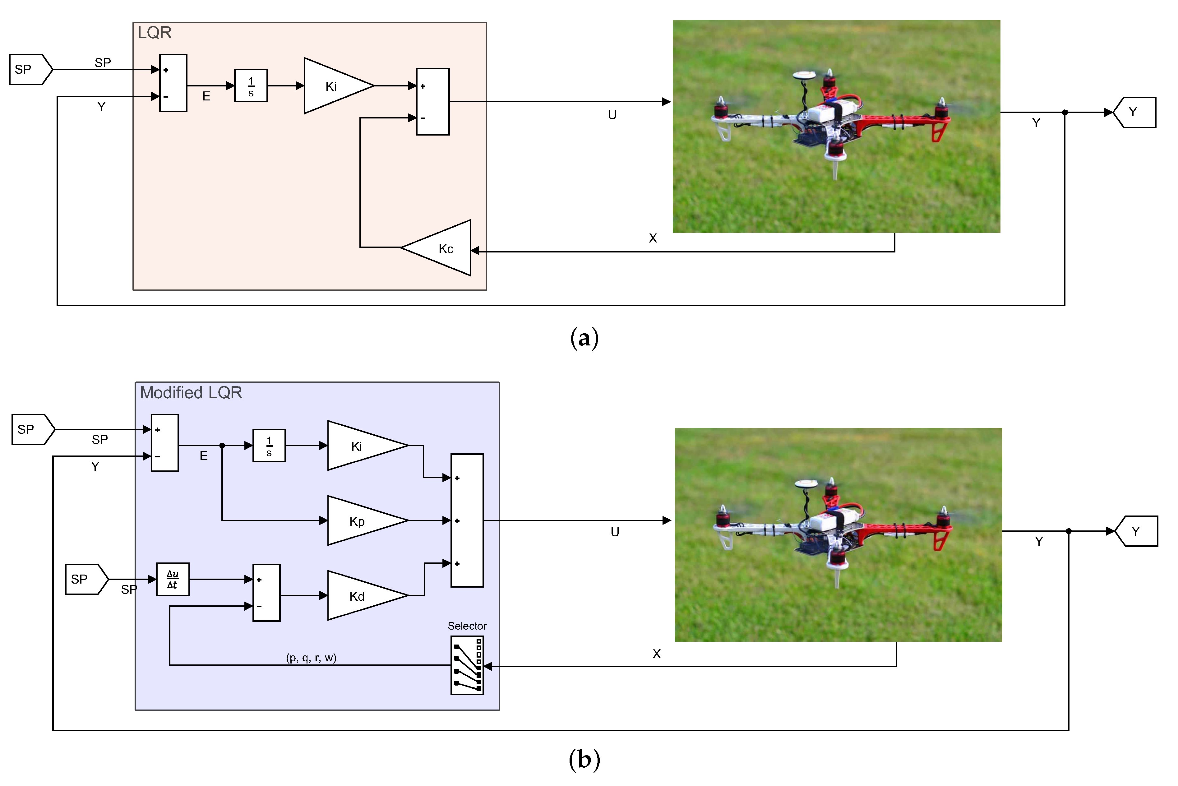
3.1. Pre-Tuning Method for Attitude and Altitude Controller

The aim of a pre-tuning procedure is to determine $Q_c$ and $R_c$ weighting matrices in (17) for which a suitable solution is obtained. For that, diagonal weighting matrices have been chosen,

$$Q_c=diag(q_{\varphi },q_{\theta },q_{\psi },q_z,q_p,q_q,q_q,q_r,q_{I\varphi },q_{I\theta },q_{I\psi },q_{Iz})$$

(21)

$$R_c=\mathrm{diag}({\rho }_{\varphi },{\rho }_{\theta },{\rho }_{\psi },{\rho }_z)$$

(22)

Taking into account experimental (computer simulations) observations of the closed-loop system, and physical meaning of the relative values used in the elements of the weighting matrices, the following relations are proposed as a starting point:

$$q_{\theta }=q_{\varphi },q_{\psi }=q_{\varphi }/7,q_z=q_{\varphi }/35$$

(23)

$$q_p=q_{\varphi }/70,q_q=q_p,q_r=q_p/5,q_w=q_p$$

(24)

$$q_{I\varphi }=q_p/2,q_{I\theta }=q_{I\varphi },q_{I\psi }=q_{I\varphi }/5,q_{Iz}=q_{I\varphi }$$

(25)

$${\rho }_{\varphi }=q_{\varphi }/4,{\rho }_{\theta }={\rho }_{\varphi },{\rho }_{\psi }={\rho }_{\varphi }/3,{\rho }_z={\rho }_{\varphi }/30$$

(26)

in this way, for a given $q_{\varphi }$ parameter value, the rest of the weighting parameters are calculated for the pre-tuning controller. In practice, due to non-linear dynamics and parameter uncertainty, it is necessary to make a fine-tuning to achieve adequate performance and robustness properties, which is made experimentally in an iterative way.

In order to analyze the properties of the proposed controller, an illustrative example is shown below, where the following tuning parameters have been adjusted experimentally,

$$Q_c=\mathrm{diag}(350,350,50,10,4,5,1,4,3,3,1,4)$$

(27)

$$R_c=\mathrm{diag}(88,88,32,3)$$

(28)

With these weighting matrices, the following state feedback matrices, $K_c$ and $K_i$, are obtained,

$$K_c=\left(\begin{array}{cccccccc}2.9394& 0.0000& -0.0000& 0.0000& 0.3174& 0.0000& 0.0000& 0.0000\\ 0.0000& 2.9408& 0.0000& 0.0000& 0.0000& 0.3401& 0.0000& 0.0000\\ 0.0000& 0.0000& 0.5024& 0.0000& 0.0000& 0.0000& 0.1542& 0.0000\\ 0.0000& 0.0000& 0.0000& 2.7333& 0.0000& 0.0000& 0.0000& 2.8867\end{array}\right)$$

(29)

$$K_I=\left(\begin{array}{cccc}0.1846& 0.0000& -0.0000& 0.0000\\ 0.0000& 0.1846& 0.0000& 0.0000\\ 0.0000& 0.0000& 0.0079& -0.0000\\ 0.0000& -0.0000& -0.0000& 1.2247\end{array}\right)$$

(30)

In order to analyze the effect of the modified LQR control law, in Figure 4 we show a comparison between the time response of the linearized system employing the conventional control law (15) and the proposed control law (19) in this paper. In both cases the initial state vector ${\mathbf{x}}_i^T\left(0\right)=(0.1,-0.3,\pi ,-1,0,0,0,0)$, is expressed in the International System of Units. As can be seen, the control law (19) achieves a significantly faster time response.

The proposed controller can be interpreted as a multivariable PID controller for a MIMO (4 × 4) system, taking into account that the $K_c$ matrix can be expressed as

$$\begin{array}{cc}\hfill K_c& =\left[K_P{K}_D\right]\hfill \\ \hfill K_P=\left(\begin{array}{cccc}2.9394& 0.0000& -0.0000& 0.0000\\ 0.0000& 2.9408& 0.0000& 0.0000\\ 0.0000& 0.0000& 0.5024& 0.0000\\ 0.0000& 0.0000& 0.0000& 2.7333\end{array}\right)& ,K_D=\left(\begin{array}{cccc}0.3174& 0.0000& 0.0000& 0.0000\\ 0.0000& 0.3401& 0.0000& 0.0000\\ 0.0000& 0.0000& 0.1542& 0.0000\\ 0.0000& 0.0000& 0.0000& 2.8867\end{array}\right)\hfill \end{array}$$

(31)

where the respective $K_P$, $K_D$ (29) and $K_I$ (30) matrices are practically diagonal matrices, and therefore they can be approximated by

$$K_P=\left(\begin{array}{cccc}{K}_{P_{\varphi }}& 0& 0& 0\\ 0& K_{P_{\theta }}& 0& 0\\ 0& 0& K_{P_{\psi }}& 0\\ 0& 0& 0& K_{P_z}\end{array}\right),K_I=\left(\begin{array}{cccc}{K}_{I_{\varphi }}& 0& 0& 0\\ 0& K_{I_{\theta }}& 0& 0\\ 0& 0& K_{I_{\psi }}& 0\\ 0& 0& 0& K_{I_z}\end{array}\right),K_D=\left(\begin{array}{cccc}{K}_{D_{\varphi }}& 0& 0& 0\\ 0& K_{D_{\theta }}& 0& 0\\ 0& 0& K_{D_{\psi }}& 0\\ 0& 0& 0& K_{D_z}\end{array}\right)$$

(32)

With these approximations, the PID control laws (using Laplace transform domain) for the components of the controller out vector are given by,

$$\begin{array}{cc}\hfill u_{\varphi }\left(s\right)& =K_{P_{\varphi }}{e}_{\varphi }\left(s\right)+{\displaystyle \frac{K_{I_{\varphi }}}{s}}{e}_{\varphi }\left(s\right)+s{K}_{D_{\varphi }}{e}_{\varphi }\left(s\right)\hfill \\ \hfill u_{\theta }\left(s\right)& =K_{P_{\theta }}{e}_{\theta }\left(s\right)+{\displaystyle \frac{K_{I_{\theta }}}{s}}{e}_{\theta }\left(s\right)+s{K}_{D_{\theta }}{e}_{\theta }\left(s\right)\hfill \\ \hfill u_{\psi }\left(s\right)& =K_{P_{\psi }}{e}_{\psi }\left(s\right)+{\displaystyle \frac{K_{I_{\psi }}}{s}}{e}_{\psi }\left(s\right)+s{K}_{D_{\psi }}{e}_{\psi }\left(s\right)\hfill \\ \hfill u_z\left(s\right)& =K_{P_z}{e}_z\left(s\right)+{\displaystyle \frac{K_{I_z}}{s}}{e}_z\left(s\right)+s{K}_{D_z}{e}_z\left(s\right)\hfill \end{array}$$

(33)

where $e_{\varphi }$, $e_{\theta }$, $e_{\psi }$, and $e_z$ are the respective tracking error signals for the controlled variables, $\varphi$, $\theta$, $\psi$ and $z_E$. Figure 5 shows block diagrams with the conventional LQR and the modified LQR control law proposed in ths work.

Once the controller output vector $\mathbf{U}$ has been calculated, the duty cycle vector, D for the PWM signals applied to motors are obtained taking into account Equation (7),

$$\mathbf{D}=M^{-1}\mathbf{U}$$

(34)

In order to implement the proposed algorithm, all state variables are needed for feedback. For that, and taking into account the characteristics of the system to control, low-cost commercial sensors characteristics are used in computer simulations based on data sheets given by manufacturers. A MARG (Magnetic, Angular Rate, and Gravity) sensors system (MPU-9250 model, with 3-axes accelerometer, rate-gyro, and magnetometer) is used for attitude and orientation measurements ([43,44]). A LIDAR (Light Detection and Ranging) is used for altitude measurement [42]. Due to bias/drift effects acting on measurements given by inertial sensors, compensation algorithms must be considered as described in the next section.

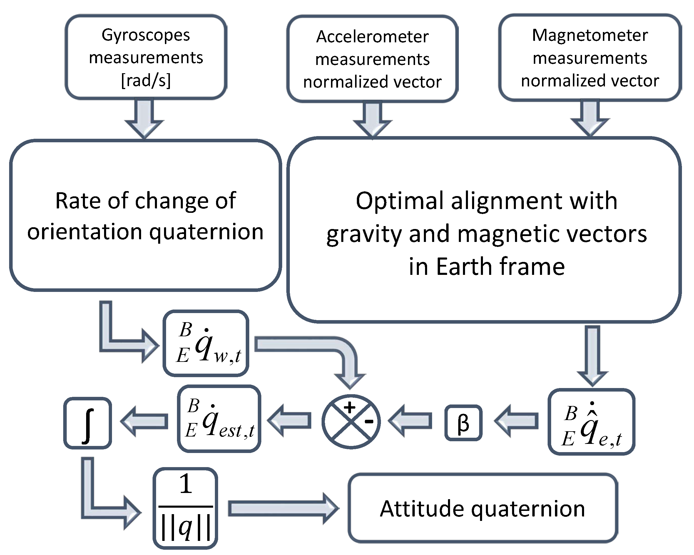
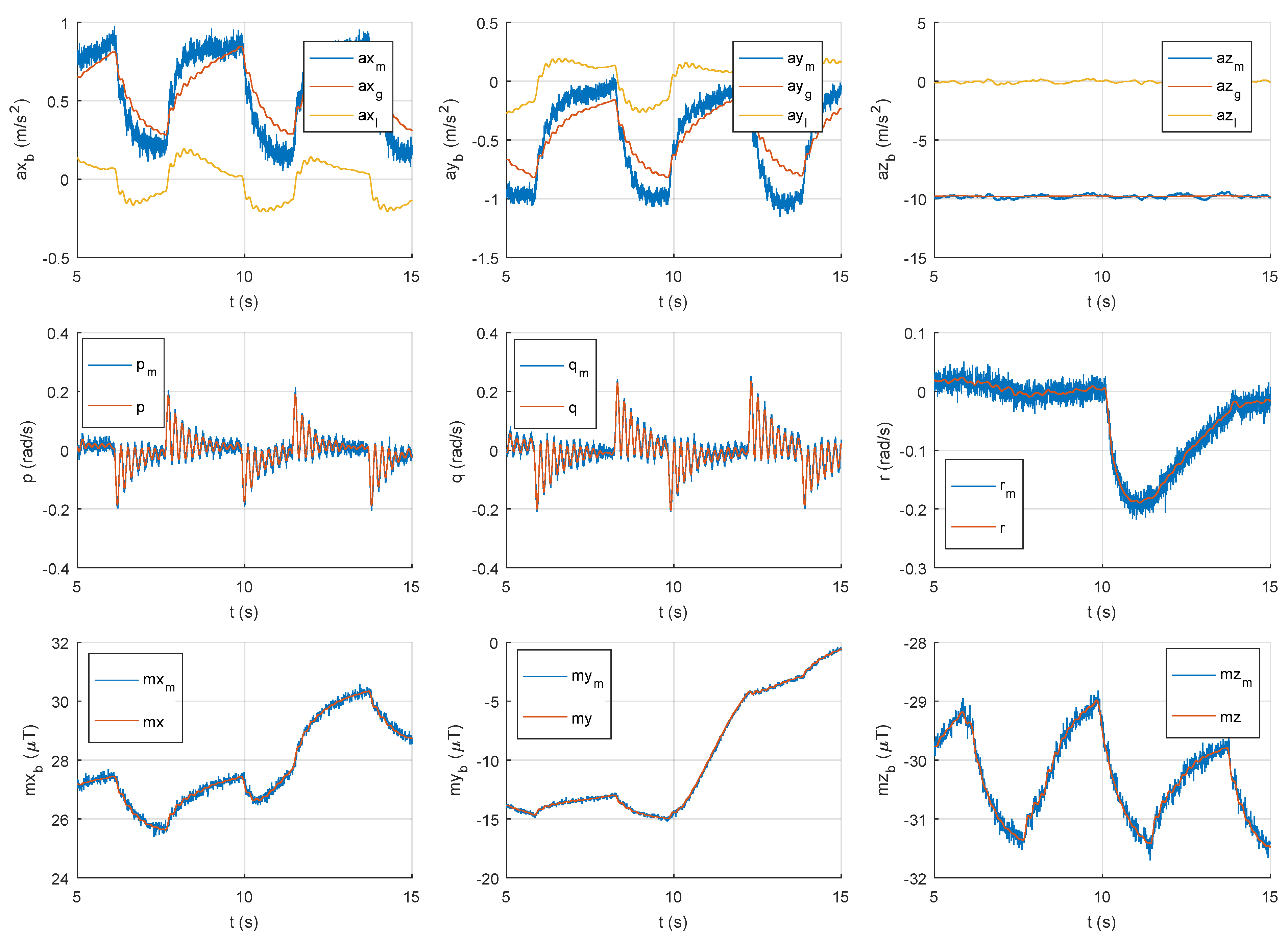
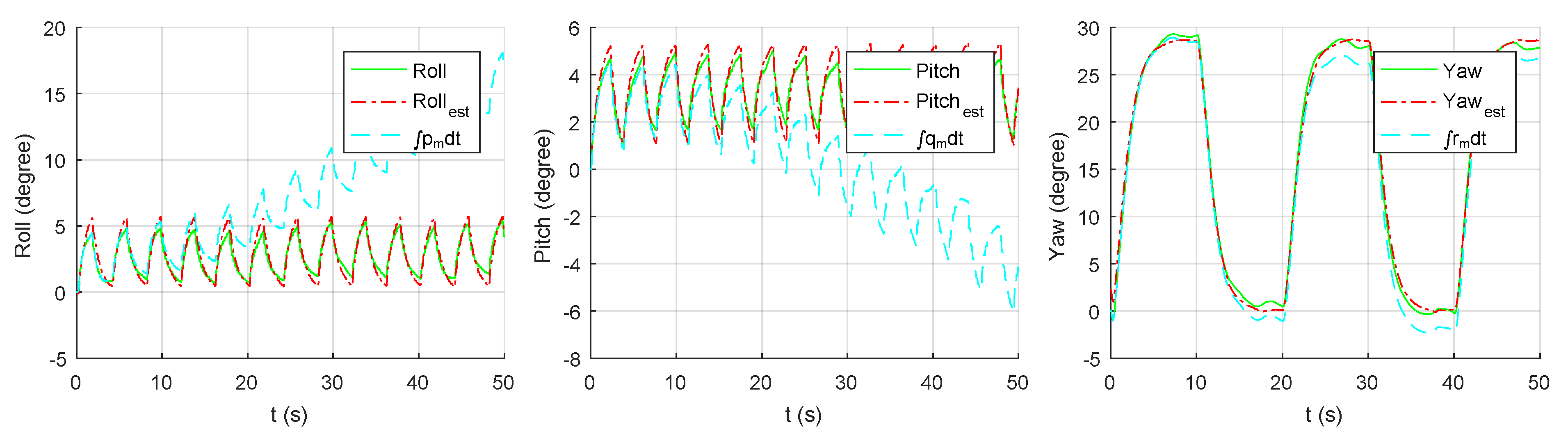
3.2. Attitude Estimation

In order to achieve proper control of the system, it is very important to have accurate enough attitude measurements. The references [50,51] compare the performance of three sensor fusion algorithms that use the MARG measurements for attitude estimation. These are an extended Kalman filter (EFK), the non-linear complementary filter (NLCF) described in [25], and the error optimization algorithm detailed in [46] based on the gradient descent method (MHV).

Table 2. RMSE (Root Mean Square Error) in dynamic conditions and compute time of the three attitude estimation algorithms considered, [51].

Parameter	EKF	MHV	NLCF
RMSE Roll [${}^{\circ }$]	4.71	4.85	5.07
RMSE Pitch [${}^{\circ }$]	1.91	2.65	2.89
RMSE Yaw [${}^{\circ }$]	5.19	5.13	5.67
Compute time [ms]	2.7	0.15	0.11

shows the relative computation times on a typical embedded system as well as the RMS errors for the three algorithms. This work uses the MHV algorithm since it has a good compromise between computation cost and estimation errors.

In each sample interval, the MHV algorithm proceeds first finding the best alignment between the gravity and Earth magnetic vectors and those measured by the accelerometer and the magnetometer, respectively. To get that optimal alignment of these two pairs of vectors despite the presence of measurement errors the MHV algorithm uses the gradient descent method. The output of this stage is a quaternion (${}_E^B{\dot{q}}_{w,t}$) presenting the rate of change of the attitude. This quaternion is then combined with the obtained from the angular velocity measured by the gyroscope (${}_E^B{\dot{q}}_{w,t}$) to calculate a better estimation (Figure 6) using

$${}_E^B{\dot{q}}_{est,t}={}_E^B{\dot{q}}_{w,t}-\beta {}_E^B{\dot{\widehat{q}}}_{e,t},$$

(35)

where $\beta$ is an adjustable weighting factor representing the gyroscope measurement error expressed as the magnitude of a quaternion derivative. The algorithm also copes with the effects of magnetic disturbances and the bias present in the gyroscope.

The angular velocity vector (p, q, r) is supposed to be taken directly from the gyroscope output and, for simulation purposes, is degraded with the noise levels stated in the datasheet [43].

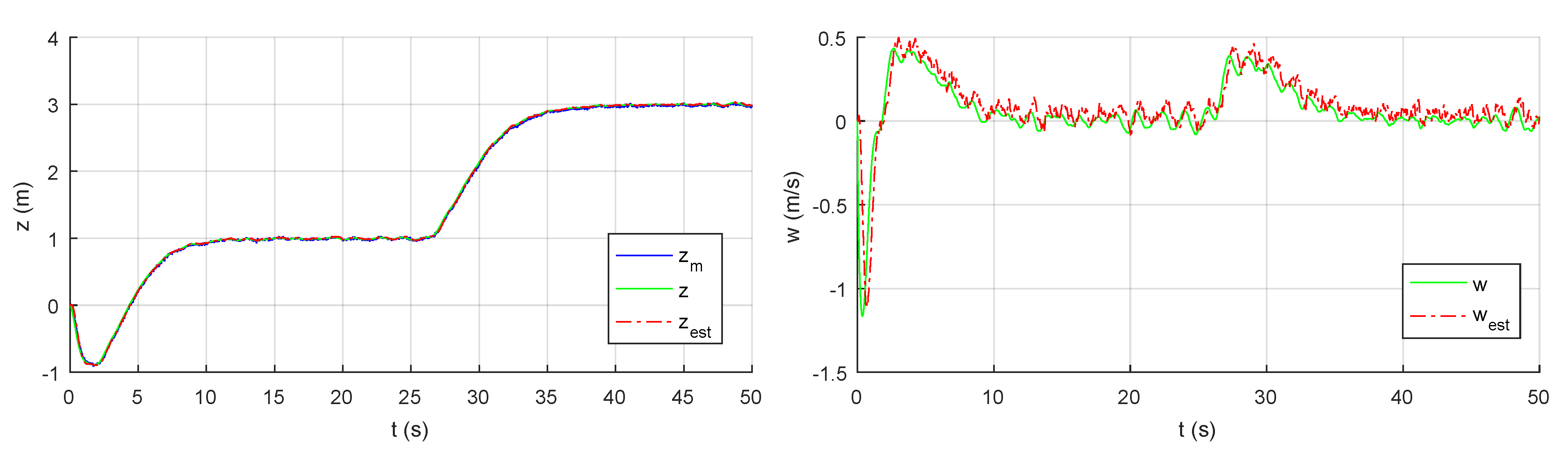
3.3. Estimation of Linear Velocity and Position in Axis $z_E$

The sensor LIDAR-LITE [42] gives a measurement from the quadrotor to ground, which can be used for estimating the vertical velocity and position. For that, taking into account the model given in (6), only the equations corresponding to ${\dot{z}}_E$ and $\dot{w}$ are considered, and it is supposed that $\varphi$ and $\theta$ take values next to zero (which is a good approximation for hover manoeuvre); with what turns out Equation (36).

$$\begin{array}{cc}\hfill \dot{w}& ={\displaystyle \frac{1}{m}}(U_z-K_{dz}w\left|w\right|)-g\hfill \\ \hfill {\dot{z}}_E& =w\hfill \end{array}$$

(36)

If (36) is linearized for hover condition ($w_{eq}=0$, $z_{eq}=0$, $U_{z_{eq}}$), a linear Kalman filter (KBF) can be used for $w,z_E$ estimation. Covariance matrices, ($Q_o,R_o$) must be adjusted to obtain a satisfactory KBF. For that, an experimental iterative procedure has been applied, obtaining the following matrices, where $R_o$ takes into account the noise measurement gives by [42],

$$Q_o=\left(\begin{array}{cc}200& 0\\ 0& 0.001\end{array}\right),R_o=0.05$$

(37)

The stationary observer gain matrix, $K_o$, can be obtained solving the corresponding observer algebraic Riccati equation (AREo) [40,48,49]. In this way, results in an LQG controller, and the complete attitude-altitude controller is a combination of LQR (for attitude control) and LQG controller (for altitude control), called, in this work, LQR/LQG. A block diagram with the complete structure of the control system is shown in Figure 7.

4. Horizontal Position Controller

Although the purpose of this article is to design a control system for the attitude and altitude (AAC) of a quadrotor, a horizontal position control (HPC) loop is included below in order to test the complete system when the attitude set-point is generated by an additional control loop whose objective is to control the position with respect to the horizontal plane. For that two scalars (SISO) PID controllers are used. The tuning of these PIDs are out of the objectives of this paper, and they are only used for testing the AAC integrated with an external control loop. As it is shown in Figure 7, the PID controllers for HPC generate as control signals the set-points for ${\varphi }_{SP}$ and ${\theta }_{SP}$ for the AAC. The output magnitudes of the set-points generate by the PIDs of the HPC are limited to avoid unnecessary pitch and roll angles, as it is shown in Figure 7. The blocks indicated as Filters correspond to first order low-pass filters used for smoothing the set-point changes sent to the controllers.

Equation (38) shows the control laws generated by the PIDs with filter to derivative action, employing the Laplace transform notation. Controllers parameters have been obtained experimentally, and are given in

Table 3. Coefficients of the position controller.

	${\mathit{K}}_{\mathit{P}}$	${\mathit{K}}_{\mathit{I}}$	${\mathit{K}}_{\mathit{D}}$	${\mathit{\tau }}_{\mathit{f}\mathit{D}}\left[\mathit{s}\right]$
$S{P}_{\varphi }$	−0.050	−0.0025	−0.08	1
$S{P}_{\theta }$	0.050	0.0025	0.08	1

(the negative sign is due to the sign criteria used for $\varphi$ and $y_B$, see Figure 2).

$$\begin{array}{cc}\hfill S{P}_{\varphi }\left(s\right)& =K_P{e}_{y_B}\left(s\right)+{\displaystyle \frac{K_I}{s}}{e}_{y_B}\left(s\right)+{\displaystyle \frac{K_{D}s}{{\tau }_{fD}s+1}}{e}_{y_B}\left(s\right)\hfill \\ \hfill S{P}_{\theta }\left(s\right)& =K_P{e}_{x_B}\left(s\right)+{\displaystyle \frac{K_I}{s}}{e}_{x_B}\left(s\right)+{\displaystyle \frac{K_{D}s}{{\tau }_{fD}s+1}}{e}_{x_B}\left(s\right)\hfill \end{array}$$

(38)

where $e_{x_B}$ and $e_{y_B}$ are the error components of the horizontal position vector (${\mathbf{e}}_H$) which are referenced to the body-axis reference system.

The horizontal positioning error can be referenced with respect to the body-axes reference system, ${\mathbf{e}}_H$($e_{x_B}$, $e_{y_B}$), as well as to the Earth-axes reference system, ${\mathbf{e}}_H$($e_{x_E}$, $e_{y_E}$). For small values of $\varphi$ and $\theta$ angles, the relation between the horizontal coordinates is given by,

$$\left(\begin{array}{c}{e}_{x_B}\\ e_{y_B}\end{array}\right)=\left(\begin{array}{cc}cos\left(\psi \right)& sin\left(\psi \right)\\ -sin\left(\psi \right)& cos\left(\psi \right)\end{array}\right)\left(\begin{array}{c}{e}_{x_E}\\ e_{y_E}\end{array}\right)$$

(39)

Horizontal Position Estimation

The horizontal position estimation of the quadrotor derives from a CMOS optical flow camera model PX4FLOW [45] pointing down. This camera computes a displacement vector utilizing the correlation between successive images, so its output is expressed in pixels units and not in real units. To compute the truth velocity is necessary to take into account the focal length of the camera lens as well as the distance from the camera to the floor, or altitude, that is already available from the LIDAR, as is shown in Equation (40). Also, the horizontal velocity has to be rotated (41) taking into account the $\psi$ angle estimated previously to refer it to the Earth frame. Then, the horizontal velocity is integrated to get the final horizontal position in that frame ($x_E,y_E$).

$$\left(\begin{array}{c}{v}_{x_B}\\ v_{y_B}\end{array}\right)=\left(\begin{array}{c}{v}_x\\ v_y\end{array}\right){\displaystyle \frac{z}{f}}$$

(40)

where z is the distance to the floor and f is the focal distance of the camera lens. The manufacturer states that the average error in the camera output is zero, so the position measurement drift should be negligible.

$$\left(\begin{array}{c}{v}_{x_E}\\ v_{y_E}\end{array}\right)=\left(\begin{array}{cc}cos\left(\psi \right)& -sin\left(\psi \right)\\ sin\left(\psi \right)& cos\left(\psi \right)\end{array}\right)\left(\begin{array}{c}{v}_{x_B}\\ v_{y_B}\end{array}\right)$$

(41)

5. Results

This section presents the results obtained, in a realistic simulation scenario, when analyzing the LQR/LQG controller modified for the attitude and the altitude proposed in this paper. For this purpose, an analysis of the performance of this control system is carried out by applying it to the AEM model of the quadrotor. The non-linear AEM model, (1) and (2), also takes into account: rotor dynamics (3), measurement errors [42,43,44,45], the effect of estimation algorithms (MHV and KBF) and the effect of adding an external control loop for the horizontal position (38) of the quadrotor. This framework is illustrated in Figure 7, which shows the interaction between measurements provided by sensors, estimation algorithms, and controllers. It should be mentioned that in all the simulations presented the numerical integration method of Runge-Kutta of fourth order with an integration step of $0.1$ ms has been used. The estimation (MHV and Kalman filter) and control algorithms are executed at a frequency of 400 Hz in simple arithmetic precision. The discretization of the controllers and the Kalman filter is carried out using the Euler backward method, and $\beta =0.01$ is used in the MHV algorithm for fusion of sensor data. To conclude, a robustness analysis of the attitude and altitude control system to parametric uncertainty and to different types of external disturbances has been realized.

Before the attitude and altitude control performances are analysed, the MARG MPU-9250 sensor modelling is shown in Figure 8. As can be seen, all measurements are affected by noise and bias levels according to the values indicated by the manufacturer [43]. In addition, in the case of accelerometers, the measurement provided ($a{x}_m$) is affected by both gravity ($a{x}_g$) and the linear accelerations experienced by the quadrotor ($a{x}_l$). This consideration has a negative effect on the estimation of the attitude made by the MHV algorithm, which can be seen in Figure 9. As a comparison, this figure also shows the result of integrating the angular velocities provided by the MARG directly to estimate the attitude. This integration diverges with time due to the bias effect present in the measured angular velocities ($p_m$, $q_m$, $r_m$). On the other hand, the Kalman Filter for altitude and linear velocity w gets to estimate these state variables accurately, see Figure 10. This is in part due to the quality of the measurements provided by the sensor Lidar-Lite [42]. Once the estimated/measured state vector is presented, it can be pointed out that the most negative effect is present in the attitude estimation; the attitude controller must be robust to the coupling presented between the estimate of the angles ($\varphi$, $\theta$) and the linear accelerations experienced by the quadrotor.

Using the state vector used for the attitude and altitude controller feedback presented here, the results obtained when applying this controller to the AEM mathematical model are shown. In Figure 11 it can be seen how the modified LQR/LQG control shows that the system follows the setpoints requested for ($\varphi$, $\theta$, $\psi$, z) adequately, despite measurement errors (Figure 8), estimation errors (Figure 9 and Figure 10) and uncertainty in the AEM model with respect to the linear design model. It should be noted that for both attitude and altitude, the error between the estimated variable and the requested setpoint is quite small ($\pm 0.2$ degrees for ${\varphi }_{est}$ and ${\theta }_{est}$). Therefore, if sensors and/or estimation algorithms of superior performance are available, the following of setpoints carried out by this controller would have a considerable improvement margin. The duty cycles (D) generated by the modified LQR/LQG controller to get the above tracking are shown in Figure 12.

On the other hand, most high-level applications of SUAV systems require the vehicle to be able to track position commands in space or maintain static positions. Therefore, it is necessary to validate the attitude and altitude controller proposed in this paper by adding an external control loop (38) for the horizontal position of the system. As shown in Figure 13, the closed-loop system resultant gets a satisfactory tracking of the setpoints demanded by the positions ($x_E$, $y_E$, $z_E$). Even with the estimation errors committed by the MHV algorithm (due to the linear accelerations experienced by the system), the modified LQR/LQG control successfully follows the setpoints rapidly (${\varphi }_{sp}$ and ${\theta }_{sp}$) demanded by the horizontal position controller. Furthermore, the proposed control structure is valid for tracking complex trajectories. Figure 14 shows the position in the quadrotor space when tracking ascending circular paths. It can be seen that despite the coupling of the system and the errors present in the estimates and measurements, the results obtained can be considered satisfactory in terms of stabilization and setpoint tracking, although they can be improved by fine-tuning the controllers.

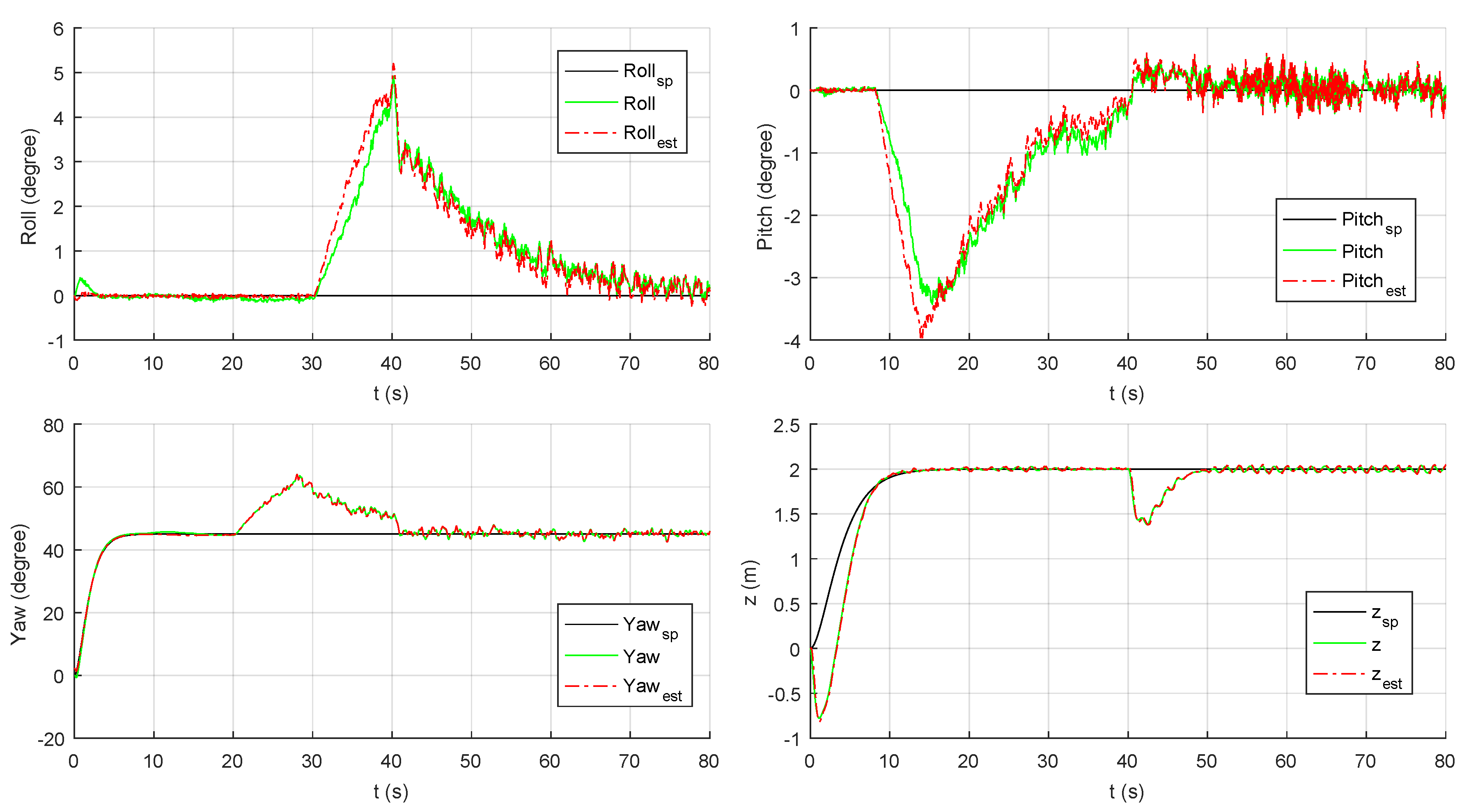
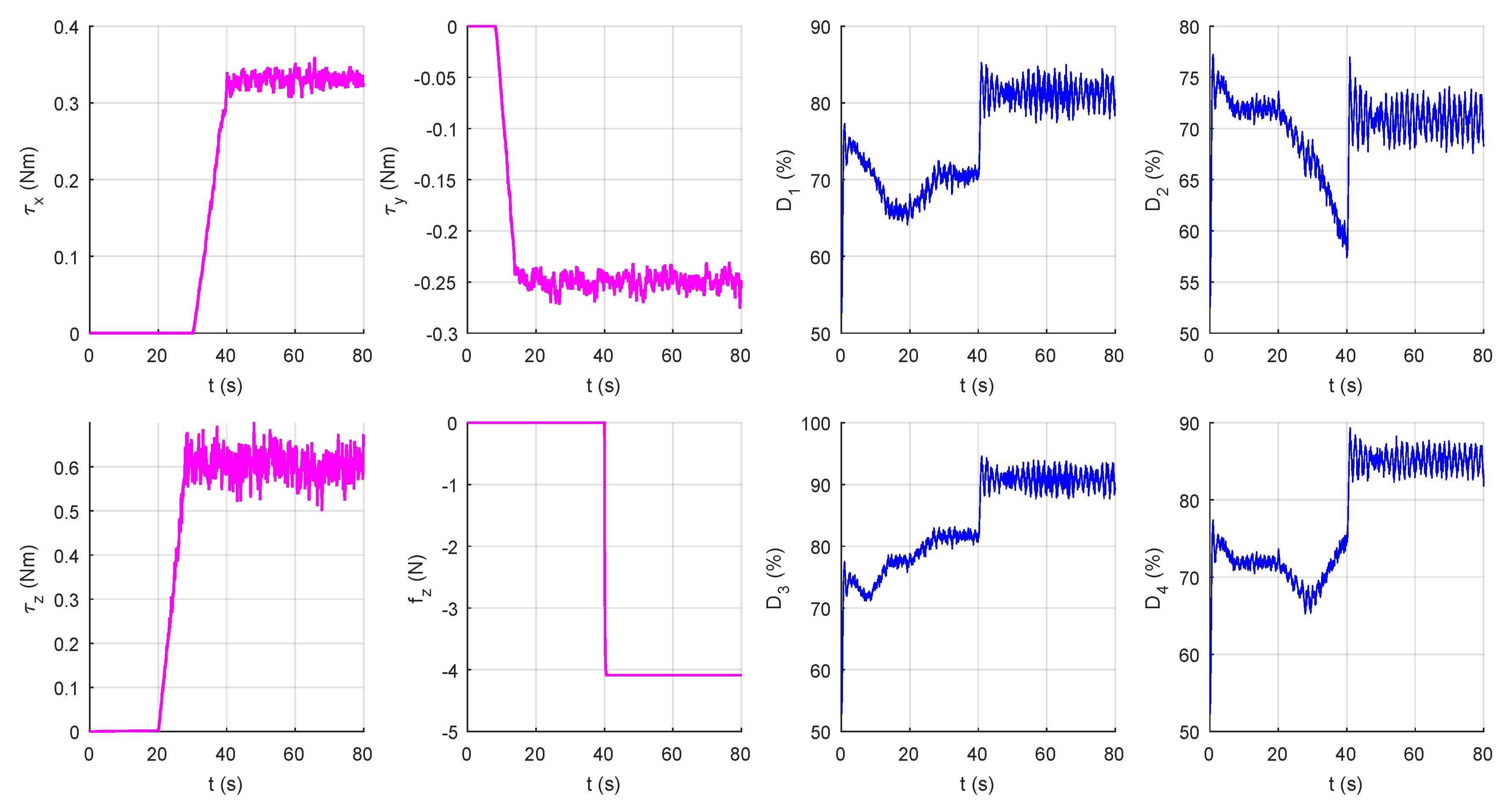
5.1. Robustness Analysis

In order to study the robustness of the modified LQR/LQG structure proposed in this work, for the pre-tuning of PID controllers applied to quadrotor systems, an analysis of attitude and altitude control is performed by adding: parametric uncertainty to the system inertia (which will determine the system response speed) and parametric uncertainty to the gain of the SISO model identified for the rotors. On the other hand, the robustness of the modified LQR/LQG control by exposing the quadrotor system to significant external disturbances (torques and forces) is also studied. Furthermore, in both cases, all measurement/estimation errors presented in the previous section are considered.

5.1.1. Parametric Uncertainty Robustness Analysis

In this analysis, the nominal inertia moments ($I_{nom}$) of the AEM model (Analysis and Evaluation Model, see Table 1) have been multiplied by a factor, $I=I_{nom}(1+\Delta I)$, which takes into account the level of uncertainty. The study focuses on this parameter because $I_x$ and $I_y$ are the ones that determine the fastest dynamics of the quadrotor and, therefore, those that affect in greater measure to the system when determining the performance of the attitude control. The study of the added uncertainty in the mass of the system has not been carried out, since this can be known with sufficient precision and does not vary with time. As result of the study,

Table 4. Performance indicators of controlled variables ($IAE$) and control effort ($IAu$) in function of parametric uncertainty added to inertia moments ($I_{add}$).

${\mathit{I}}_{\mathit{add}}$$[\mathbf{\%}]$	$\mathit{I}\mathit{A}\mathit{E}\mathit{X}$	$\mathit{I}\mathit{A}\mathit{E}\mathit{Y}$	$\mathit{I}\mathit{A}\mathit{E}\mathit{Z}$	$\mathit{I}\mathit{A}\mathit{E}\mathit{\varphi }$	$\mathit{I}\mathit{A}\mathit{E}\mathit{\theta }$	$\mathit{I}\mathit{A}\mathit{E}\mathit{\psi }$	$\mathit{I}\mathit{A}\mathit{u}$
80.0	1.0786	1.2454	5.6103	15.2990	15.2290	29.3750	257.5400
75.0	1.0408	1.1395	5.6099	14.1720	12.7410	27.7470	248.1000
62.5	1.0648	1.0532	5.6083	13.0620	10.768	26.3290	237.8200
50.0	1.1173	1.0406	5.6071	12.7620	9.9366	25.3390	233.3900
37.5	1.1384	1.0341	5.6064	12.5770	9.4105	24.5050	231.0600
25.0	1.1418	1.0277	5.6062	12.4480	9.0783	23.6990	229.8900
17.5	1.1443	1.0261	5.6061	12.4010	8.9529	23.2200	229.6400
15.0	1.1455	1.0261	5.6060	12.3910	8.9241	23.0640	229.6500
12.5	1.1467	1.0263	5.6060	12.3860	8.9038	22.9140	229.7400
10.0	1.1477	1.0266	5.6060	12.3870	8.8905	22.7650	229.9000
7.5	1.1494	1.0268	5.6060	12.3970	8.8854	22.6150	230.1600
5.0	1.1515	1.0272	5.6060	12.4110	8.8917	22.4660	230.5500
2.5	1.1532	1.0273	5.6059	12.4320	8.9092	22.3200	231.1000
0	1.1552	1.0271	5.6059	12.4540	8.9375	22.1670	231.8700
−2.5	1.1571	1.0266	5.6059	12.4720	8.9901	22.0250	232.8800
−5.0	1.1588	1.0262	5.6059	12.4890	9.0719	21.9010	234.2100
−7.5	1.1609	1.0273	5.6060	12.5200	9.1945	21.7840	235.9800
−10.0	1.1643	1.0295	5.6060	12.5830	9.3560	21.6470	238.4800
−12.5	1.1665	1.0339	5.6060	12.6990	9.5755	21.5120	242.5300
−15.0	1.1725	1.0484	5.6059	12.9250	10.0260	21.3830	251.5600
−17.5	1.1947	1.0800	5.6062	14.0740	10.8630	21.4570	272.8800
−18.5	1.2149	1.0928	5.6085	17.5760	11.1710	21.7040	316.6300
−19.5	1.1920	1.1332	5.6043	18.4920	11.7490	23.4380	331.3600

shows the values obtained when calculating the IAE (Integrated Absolute Error) of all controlled variables (x, y, z, $\varphi$, $\theta$, $\psi$) in function of the uncertainty added to the inertia moments ($I_{add}=\Delta I\times 100\%$). In addition, it records the IAu (Integrated Absolute) of the incremental variable u, which is defined as the sum of the incremental duty cycles (d) with respect to the equilibrium condition (${\mathbf{D}}_{\mathbf{eq}}$). All the simulations carried out to obtain the values listed in Table 4 are reproductions of the one shown in Figure 13 and, moreover, the time interval used for its computation is equal to the sampling time ($Tm=2.5$ ms). As visual support to the above, Figure 15 shows the variation of the IAE attitude-altitude indicators and the IAu control effort indicator.

As can be seen, the low variation of the indicators for uncertainty levels close to the nominal value ([−17.5, 17.5]%) shows that the modified LQR/LQG controller, together with the horizontal position controller, presents robust behaviour to the uncertainty added to this parameter. Furthermore, the control system achieves to stabilize the system with acceptable stationary error values ($\pm 0.5$° for attitude and $\pm 0.04$ m for position) in an uncertainty range of [−19.5, 80]%, see Figure 16. Secondly, it should be noted that the magnitude of the IAE indicators decreases considerably if these are calculated with respect to the estimated variables, see

Table 5. Performance indicators of the estimated controlled variables ($IAE$) in function of the parametric uncertainty added to inertia moments ($I_{add}$).

${\mathit{I}}_{\mathit{a}\mathit{d}\mathit{d}}$$[\mathbf{\%}]$	${\mathit{I}\mathit{A}\mathit{E}\mathit{X}}_{\mathit{e}\mathit{s}\mathit{t}}$	${\mathit{I}\mathit{A}\mathit{E}\mathit{Y}}_{\mathit{e}\mathit{s}\mathit{t}}$	${\mathit{I}\mathit{A}\mathit{E}\mathit{Z}}_{\mathit{e}\mathit{s}\mathit{t}}$	$\mathit{I}\mathit{A}\mathit{E}{\mathit{\varphi }}_{\mathit{e}\mathit{s}\mathit{t}}$	$\mathit{I}\mathit{A}\mathit{E}{\theta }_{\mathit{e}\mathit{s}\mathit{t}}$	$\mathit{I}\mathit{A}\mathit{E}{\mathit{\psi }}_{\mathit{e}\mathit{s}\mathit{t}}$
80.0	1.0540	1.1516	5.9497	10.9330	14.2230	13.5330
75.0	1.0362	1.1035	5.9494	9.2675	11.2260	13.1880
62.5	1.0460	1.0832	5.9476	6.6436	7.9389	12.3290
50.0	1.0567	1.0789	5.9458	5.3444	6.2991	11.4950
37.5	1.0709	1.0779	5.9448	4.6290	5.2787	10.6320
25.0	1.0793	1.0743	5.9443	4.2501	4.6732	9.7469
17.5	1.0849	1.0738	5.9441	4.0947	4.4447	9.2150
15.0	1.0871	1.0741	5.9441	4.0536	4.3870	9.0385
12.5	1.0895	1.0746	5.9440	4.0185	4.3410	8.8624
10.0	1.0919	1.0751	5.9440	3.9911	4.3064	8.6862
7.5	1.0941	1.0754	5.9440	3.9774	4.2820	8.5101
5.0	1.0962	1.0759	5.9440	3.9762	4.2724	8.3350
2.5	1.0982	1.0765	5.9439	3.9865	4.2806	8.1609
0	1.0995	1.0771	5.9440	4.0120	4.3068	7.9877
−2.5	1.1007	1.0777	5.9440	4.0513	4.3638	7.8161
−5.0	1.1026	1.0786	5.9440	4.1067	4.4628	7.6468
−7.5	1.1055	1.0806	5.9440	4.1940	4.6223	7.4801
−10.0	1.1090	1.0824	5.9440	4.3763	4.8359	7.3095
−12.5	1.1134	1.0851	5.9442	4.7788	5.1354	7.1386
−15.0	1.1184	1.0927	5.9441	5.5396	5.7354	6.9640
−17.5	1.1398	1.1083	5.9445	7.5210	6.8205	6.8099
−18.5	1.1800	1.1204	5.9470	12.3800	7.2495	6.7940
−19.5	1.2078	1.2035	5.9431	12.8240	8.0231	6.8986

. This supports the previously mentioned, the results obtained when applying the control structure proposed in this work to the AEM model have a considerable margin of improvement if the quality of the measures/estimates is increased.

To conclude, Figure 17 shows the results obtained by adding a parametric uncertainty to: the inertia moments ($I_{add}=-10\%$) and the gains of the SISO models identified for the rotors, $\Delta K_R=(4,-6,3.2,-2.9)\%$. As can be seen, the modified LQR/LQG controller and the position controller follow the setpoints demanded in an acceptable way, although they present an increase in overshoot and tracking error than the one obtained in Figure 13 (under the absence of added parametric uncertainty). The negative value chosen for the uncertainty added to the moments of inertia has been fixed to obtain an unfavourable situation. Since, as shown by the indicators in Table 4 and Table 5 and in Figure 15, lower inertia moments make the system faster and, therefore, if the control system is not adjusted, its performance decreases.

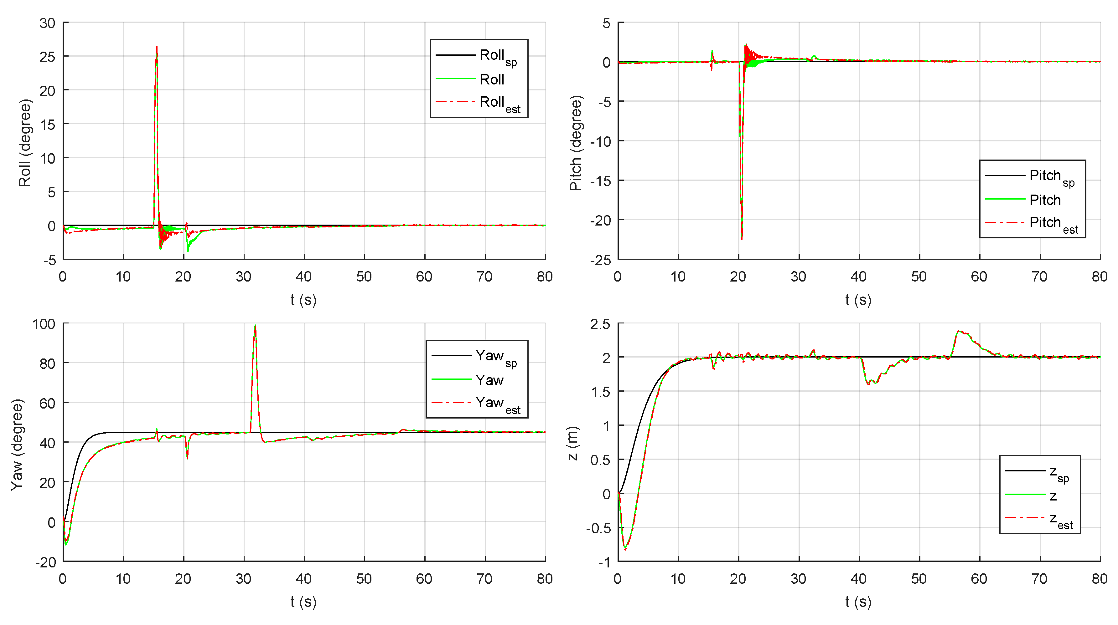
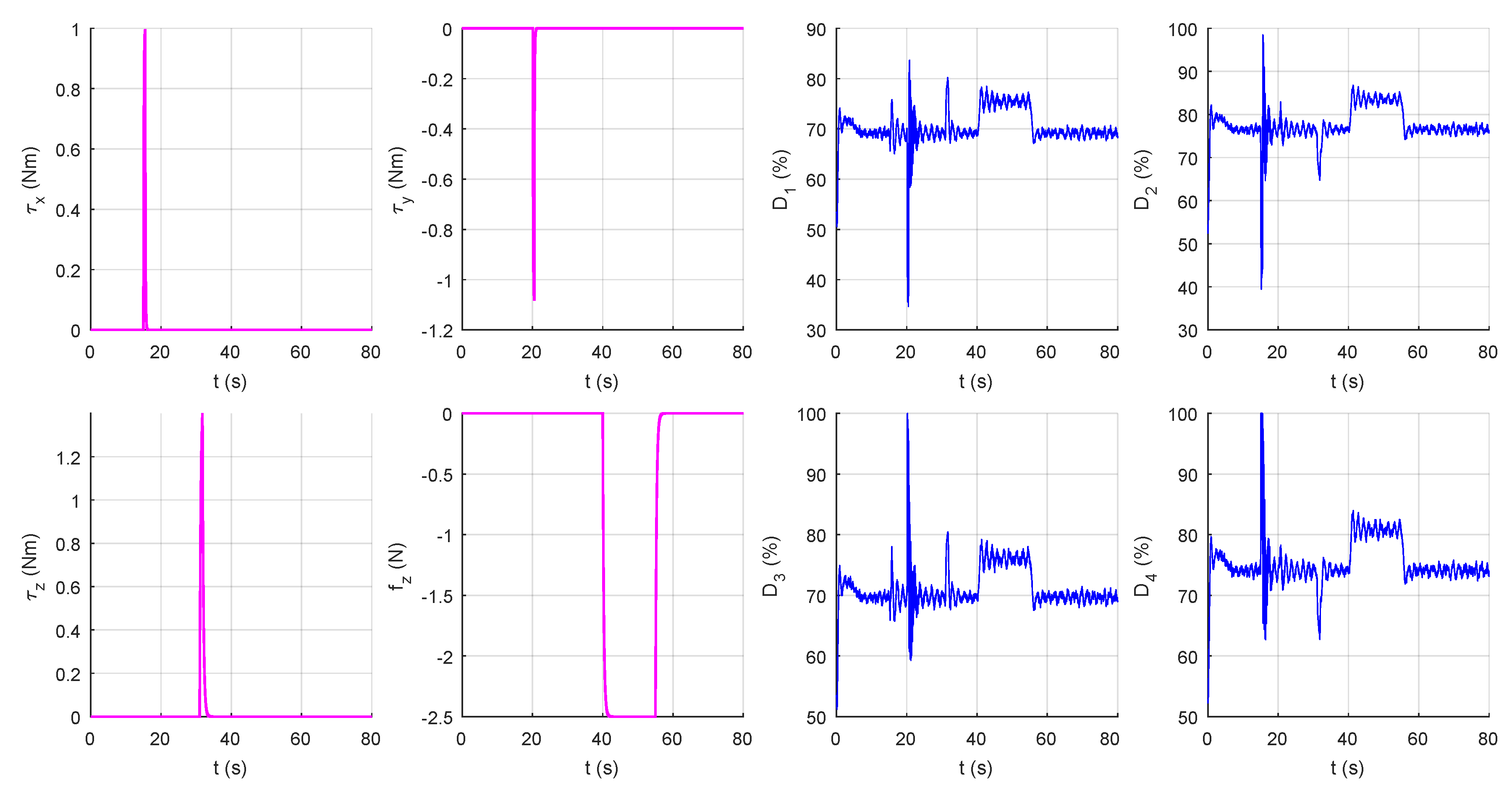
5.1.2. External Disturbance Robustness Analysis

In this section, the robustness to significant external disturbances of the modified LQR/LQG control proposed in this paper is studied. First, a scenario in which the AEM model is subjected to external torques that increase until a constant value is established, adding to these torques a stochastic component (simulating a continuous wind). Furthermore, in the same scenario, a significant increase in weight is applied to the quadrotor (one-third of its weight) in order to simulate a manoeuvre in which the quadrotor system would elevate a load outdoors for then transport it. The results obtained when carrying out the hover manoeuvre in this scenario are presented in Figure 18.

As shown in the figure above, external disturbances are successfully rejected by the attitude and altitude controller, although the rejection time could be improved if fine-tuning to the integral action of the controllers is carried out. It should be added that the stochastic component of the disturbances increases the oscillation in the controlled variables. Especially in the angles $\varphi$ and $\theta$, although in this scenario this oscillation can be considered admissible, since it is bounded between $[-0.5,0.5]$ degrees. The duty cycles generated by the modified LQR/LQG control system and the applied external disturbances are shown in Figure 19.

Finally, another scenario in which the quadrotor system is exposed to occasional external disturbances (of significant magnitude) while performing the hover manoeuvre is considered. This scenario can occur in obstacle avoidance and path planning missions, in which SUAV systems are often used. Specifically, the external torques and forces to which the AEM model is exposed could be the result of punctual collisions with different obstacles, as a result of a fault in the avoidance system, see Figure 20 and Figure 21. In addition, in order to create an unfavorable scenario, an uncertainty of $I_{add}=-10\%$ has been added to the inertia moments of the AEM model and an uncertainty $\Delta K_R=(-2.5,2,-2.3,-2.2)\%$ is also added to the gains of the SISO models identified for the rotors.

In this last scenario, the magnitude of the external punctual torques makes that the system deviates considerably (25 and $-22.5$ degrees in the angles $\varphi$ and $\theta$, respectively) from the equilibrium position hover, for which the modified LQR/LQG control has been designed. Moreover, the punctual torque on the $z_B$ axis causes an undesired turn of 45 degrees on the $\psi$ angle. However, the attitude control system is able to correct the effect of these punctual disturbances (shown in Figure 21) and return the system to its equilibrium point (hover). It should be added that the altitude control also achieves to reject the force maintained for 16 s on the $z_E$ axis. To reject this set of disturbances, the controller generates the duty cycles for the PWM signals shown in Figure 21. Therefore, the robustness of the modified LQR/LQG controller has been checked under the presence of significant punctual disturbances and added parametric uncertainty.

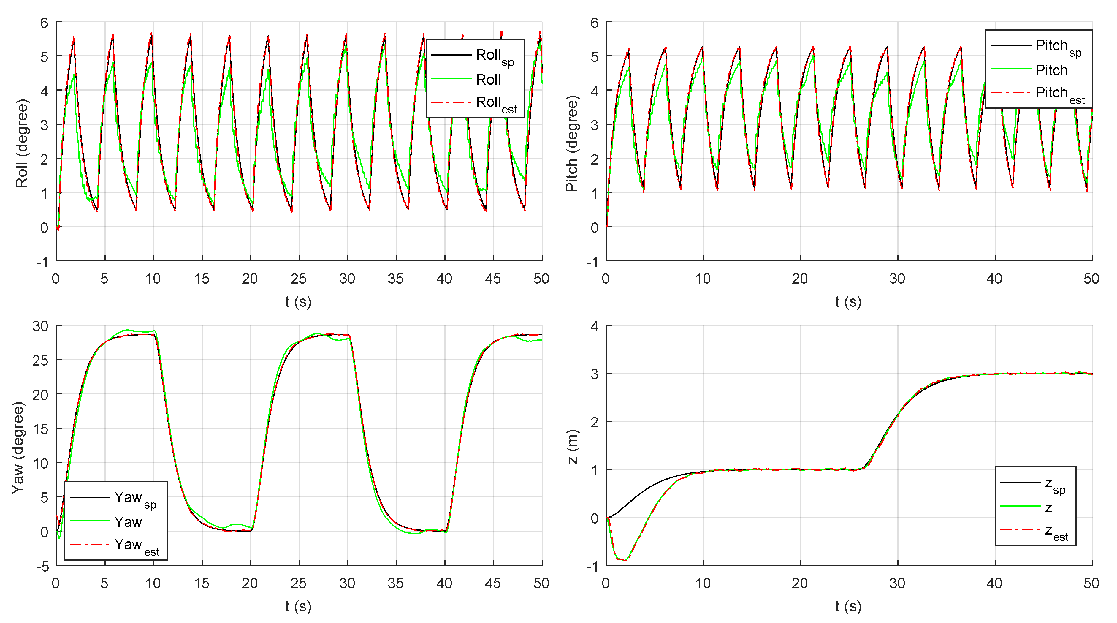
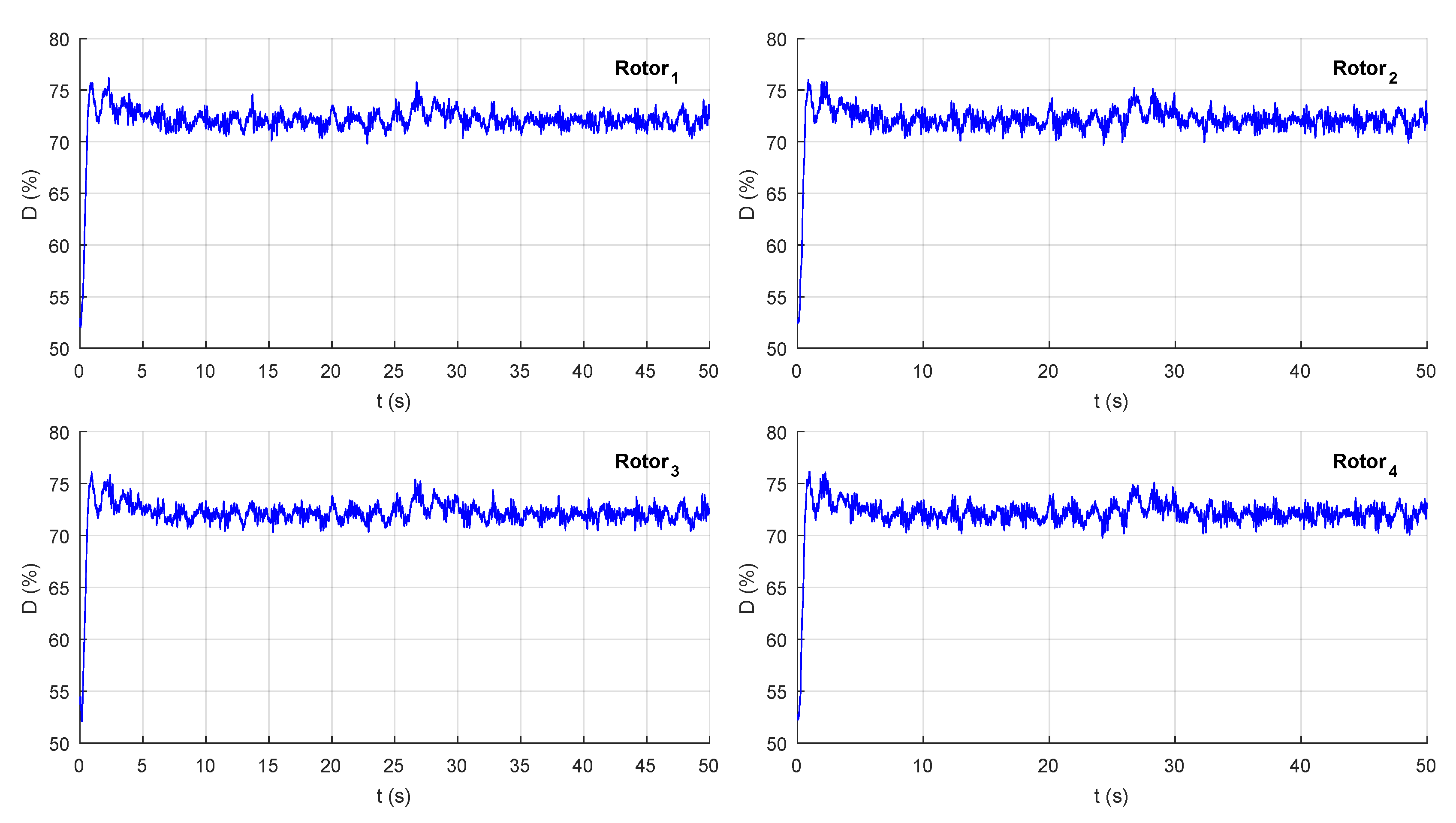
5.2. First Pre-Tuning Tests on the Real System

In order to validate the pre-tuning method proposed in this work, the initial results obtained when implementing the set of algorithms presented in the real quadrotor DJI F-450 are shown. Note that it is not the object of this work to compare the proposed method with alternative methods; this will be studied in future works. In this section, we only want to show the validity of the proposed method through its implementation in a real system. The results obtained can be improved by fine-tuning. With the limitations of these real tests established, it should be added that the embedded system has been implemented on the PCB whose schematic with the main parts is shown in Figure 22.

Figure 23 shows the behaviour of the multirotor for setpoint changes in altitude (where $z_{sp}$ and $z_{est}$ denote setpoint and estimated variable, respectively). An acceptable average tracking error is obtained for a pre-tuning stage, and the maximum transient error is limited to $\pm 0.07$ m.

Figure 24 shows the attitude ($\varphi$, $\theta$, $\psi$) of the quadrotor during takeoff (where the subindex ${}_{SP}$ and ${}_{est}$ denote setpoint and estimated variable, respectively). As it can be seen, the modified LQR controller needs a few seconds to get that the quadrotor follows the attitude setpoints demanded. After this transitory, the system follows the demanded setpoints with a tracking error bounded between $\pm 2$ degrees. These results are less favorable than those obtained with the simulated model but could be improved by fine-tuning the controller. This is due to the fact that there will always be differences between the real system and the simulation. These differences are mainly due to the uncertainty in the model used for design, as well as possible disturbances acting on the system. Finally, [52] presents a video in which the real quadrotor system is affected by significant external disturbances. As can be seen in this video, the pre-tuning method proposed in this work obtains a robust attitude and altitude controller to significant external disturbances.

6. Conclusions

A method for pre-tuning a multivariable PID controller for a quadrotor attitude and altitude control has been proposed, which is based on LQR/LQG theory, using a modified structure of the LQR, where the state feedback algorithm employs the tracking error vector instead of the state vector. The proposed method uses only one pre-tuning parameter, which easily facilitates the controller design. Realistic computer simulations have been carried out using a nonlinear mathematical model of the DJI-F450 quadrotor, considering parametric uncertainty and external disturbances acting at the plant input. Madgwick’s algorithm and a Kalman filter have been used for data fusion and estimating state variables using data from MARG, LIDAR, and optical flow camera, which have been simulated using data sheets provided by manufactures. Simulation results show that the proposed method design gives MIMO PID controllers which are robust in the face of uncertainties and external disturbances acting at plant input.

References

1. Valavanis, K.; Vachtsevanos, G.J. Handbook of Unmanned Aerial Vehicles, 1st ed.; Springer: Dordrecht, The Netherlands, 2015; ISBN 978-90-481-9706-4. [Google Scholar]
2. Lozano, R. Unmanned Aerial Vehicles: Embedded Control, 1st ed.; Wiley-ISTE: Hoboken, NJ, USA, 2010; ISBN 1848211279. [Google Scholar]
3. Nonami, K.; Kendoul, F.; Suzuki, S.; Wang, W.; Nakazawa, D. Autonomous Flying Robots: Unmanned Aerial Vehicles and Micro Aerial Vehicles, 1st ed.; Springer: Tokyo, Japan, 2010; ISBN 978-4-431-53855-4. [Google Scholar]
4. Mahony, R.; Kumar, V.; Corke, P. Multirotor Aerial Vehicles. IEEE Robot. Autom. Mag. 2012, 19, 20–32. [Google Scholar] [CrossRef]
5. Peña, M.; Vivas, C.E.; Rodriguez, C. Modelamiento Dinámico y control LQR de un Quadrotor. AVANCES Investig. Ing. 2010, 13, 71–86. [Google Scholar] [CrossRef]
6. Li, J.; Li, Y. Dynamic Analysis and PID Control for a Quadrotor. In Proceedings of the IEEE International Conference on Mechatronics and Automation, Beijing, China, 7–10 August 2011; pp. 573–578. [Google Scholar]
7. Xiong, J.; Zheng, E. Optimal Kalman Filter for state estimation of a quadrotor UAV. Opt. Int. J. Light Electron. Opt. 2015, 126, 2862–2868. [Google Scholar] [CrossRef]
8. Fernando, H.C.T.E.; De Silva, A.T.A.; De Zoysa, M.D.C.; Dilshan, K.A.D.C.; Munasinghe, S.R. Modelling, Simulation and Implementation of a Quadrotor UAV. In Proceedings of the IEEE 8th International Conference on Industrial and Information Systems, Peradeniya, Sri Lanka, 17–20 December 2013; pp. 207–212. [Google Scholar]
9. Lozano, Y.; Gutiérrez, O. Design and Control of a Four-Rotary-Wing Aircraft. IEEE Lat. Am. Trans. 2016, 14, 4433–4438. [Google Scholar] [CrossRef]
10. Castillo, P.; Lozano, R.; Dzul, A. Stabilization of a Mini Rotorcraft with Four Rotors. Experimental implementation of linear and nonlinear control laws. IEEE Control Syst. Mag. 2005, 25, 45–55. [Google Scholar] [CrossRef]
11. Xiong, J.; Zheng, E. Position and attitude tracking control for a quadrotor UAV. ISA Trans. 2014, 53, 725–731. [Google Scholar] [CrossRef] [PubMed]
12. Rubio, J.D.J.; Cruz, J.H.P.; Zamudio, Z.; Salinas, A.J. Comparison of Two Quadrotor Dynamic Models. IEEE Lat. Am. Trans. 2014, 12, 531–537. [Google Scholar] [CrossRef]
13. Reinoso, M.; Minchala, L.I.; Ortiz, J.P.; Astudillo, D.; Verdugo, D. Trajectory tracking of a quadrotor using sliding mode control. IEEE Lat. Am. Trans. 2016, 14, 2157–2166. [Google Scholar] [CrossRef]
14. Gómez, M.; Pérez, M.; Puentes, C. MÉCANICA DEL VUELO, 2nd ed.; Ibergarceta Publicaciones S.L.: Madrid, Spain, 2012; ISBN 978-84-15452-01-0. [Google Scholar]
15. Altug, E.; Ostrowski, J.P.; Mahony, R. Control of a Quadrotor Helicopter Using Visual Feedback. In Proceedings of the 2002 IEEE International Conference on Robotics and Automation, Washington, DC, USA, 11–15 May 2002; pp. 72–77. [Google Scholar]
16. Azfar, A.Z.; Hazry, D. A Simple Approach on Implementing IMU Sensor Fusion in PID Controller for Stabilizing Quadrotor Flight Control. In Proceedings of the IEEE 7th International Colloquium on Signal Processing and Its Applications, Penang, Malaysia, 4–6 March 2011; pp. 28–32. [Google Scholar]
17. Lee, K.U.; Kim, H.S.; Park, J.B.; Choi, Y.H. Hovering Control of a Quadrotor. In Proceedings of the International Conference on Control, Automation and Systems, JeJu Island, Korea, 17–21 October 2012; pp. 162–167. [Google Scholar]
18. Zhih, C.C.; Kumar, S.; Ragavan, V.; Shanmugavel, M. Development of a Simple, Low-cost Autopilot System for Multi-rotor UAVs. In Proceedings of the IEEE Recent Advances in Intelligent Computational Systems, Trivandrum, India, 10–12 December 2015; pp. 285–289. [Google Scholar]
19. Tang, Y.; Li, Y.; Ma, T. Design, Implementation and Control of a Small-scale UAV Quadrotor. In Proceedings of the World Congress on Intelligent Control and Automation, Shenyang, China, 29 June–4 July 2014; Volume 183, pp. 2364–2369. [Google Scholar]
20. Burri, M.; Dätwiler, M.; Achtelik, M.W.; Siegwart, R. Robust State Estimation for Micro Aerial Vehicles Based on System Dynamics. In Proceedings of the IEEE International Conference on Robotics and Automation, Seattle, WA, USA, 26–30 May 2015; pp. 5278–5283. [Google Scholar]
21. Oh, K.; Ahn, H. Extended Kalman Filter with Multi-frequency Reference Data for Quadrotor Navigation. In Proceedings of the International Conference on Control, Automation and Systems, Busan, Korea, 13–16 October 2015; pp. 201–206. [Google Scholar]
22. Kong, X.; Li, J.; Yu, H.; Wu, W. Robust Kalman Filtering for Attitude Estimation Using Low-cost MEMS-based Sensors. In Proceedings of the IEEE Chinese Guidance, Navigation and Control Conference, Yantai, China, 8–10 August 2014; pp. 2779–2783. [Google Scholar]
23. Gasior, P.; Bondyra, A.; Gardecki, S.; Giernacki, W. Robust estimation algorithm of altitude and vertical velocity for multirotor UAVs. In Proceedings of the 21st International Conference on Methods and Models in Automation and Robotics, Miedzyzdroje, Poland, 29 August–1 September 2016; pp. 714–719. [Google Scholar]
24. Abeywardena, D.; Kodagoda, S.; Dissanayake, G.; Munasinghe, R. Improved State Estimation in Quadrotor MAVs. IEEE Robot. Autom. Mag. 2013, 20, 32–39. [Google Scholar] [CrossRef]
25. Mahony, R.; Hamel, T.; Pflimlin, J. Nonlinear Complementary Filters on the Special Orthogonal Group. IEEE Trans. Autom. Control 2008, 53, 1203–1218. [Google Scholar] [CrossRef]
26. Almeshal, A.M.; Alenezi, M.R. A Vision-Based Neural Network Controller for the Autonomous Landing of a Quadrotor on Moving Targets. Robotics 2018, 7, 15. [Google Scholar] [CrossRef]
27. Raffo, G.V.; Ortega, M.G.; Rubio, F.R. An integral predictive/nonlinear H control structure for a quadrotor helicopter. Automatica 2010, 46, 29–39. [Google Scholar] [CrossRef]
28. Lee, K.; Choi, Y.; Park, J. Inverse Optimal Design for Position Control of a Quadrotor. Appl. Sci. 2017, 7, 907. [Google Scholar] [CrossRef]
29. Mukhopadhyay, S. PID equivalent of optimal regulator. Electron. Lett. 1978, 14, 821–822. [Google Scholar] [CrossRef]
30. Argentim, L.M.; Rezende, W.C.; Santos, P.E.; Aguiar, R.A. PID, LQR and LQR-PID on a Quadcopter Platform. In Proceedings of the International Conference on Informatics, Electronics and Vision, Dhaka, Bangladesh, 17–18 May 2012; pp. 1–6. [Google Scholar]
31. Salim, N.D.; Derawi, D.; Shah Abdullah, S.; Mazlan, S.A.; ZamZuri, H. PID plus LQR Attitude Control for Hexarotor MAV in Indoor Environments. In Proceedings of the IEEE International Conference on Industrial Technology, Busan, Korea, 26 February–1 March 2014; pp. 85–90. [Google Scholar]
32. Reyes-valeria, E.; Enriquez-caldera, R.; Camacho-lara, S.; Guichard, J. LQR Control for a Quadrotor using Unit Quaternions: Modeling and Simulation. In Proceedings of the 23rd International Conference on Electronics, Communications and Computing, Cholula, Mexico, 11–13 March 2013; pp. 172–178. [Google Scholar]
33. Khatoon, S.; Gupta, D.; Das, L.K. PID and LQR Control for a Quadrotor: Modeling and Simulation. In Proceedings of the International Conference on Advances in Computing, Communications and Informatics, New Delhi, India, 24–27 September 2014; pp. 796–802. [Google Scholar]
34. Belkheiri, M.; Rabhi, A.; Hajjaji, A.E.L.; Pégard, C.P. Different Linearization Control Techniques for a Quadrotor System. In Proceedings of the CCCA12, Marseilles, France, 6–8 December 2012; pp. 1–6. [Google Scholar]
35. Yu, B.; Zhang, Y.; Qu, Y. Fault Tolerant Control Using PID Structured Optimal Technique Against Actuator Faults in a Quadrotor UAV. In Proceedings of the International Conference on Unmanned Aircraft Systems, Orlando, FL, USA, 27–30 May 2014; pp. 167–174. [Google Scholar]
36. González-Vázquez, S.; Moreno-Valenzuela, J. A new nonlinear PI/PID controller for quadrotor posture regulation. In Proceedings of the 2010 Electronics, Robotics and Automotive Mechanics Conference (CERMA), Morelos, Mexico, 28 September–1 October 2010; pp. 642–647. [Google Scholar]
37. Alcan, G.; Unel, M. Robust hovering control of a quadrotor using acceleration feedback. In Proceedings of the 2017 International Conference on Unmanned Aircraft Systems (ICUAS), Miami, FL, USA, 13–16 June 2017; pp. 1455–1462. [Google Scholar]
38. Moreno-Valenzuela, J.; Perez-Alcocer, R.; Guerrero-Medina, M.; Dzul, A. Nonlinear PID-Type Controller for Quadrotor Trajectory Tracking. IEEE/ASME Trans. Mechatron. 2018, 23, 2436–2447. [Google Scholar] [CrossRef]
39. Dong, J.; He, B. Novel fuzzy PID-type iterative learning control for quadrotor UAV. Sensors 2019, 19, 24. [Google Scholar] [CrossRef] [PubMed]
40. Ogata, K. Ingeniería de Control Modernaê, 5th ed.; PEARSON EDUCACIÓN S.A.: Madrid, Spain, 2010; ISBN 9788483226605. [Google Scholar]
41. DJI. Available online: www.dji.com (accessed on 4 May 2015).
42. PulsedLight. LIDAR-Lite Operating Manual; Rev 1.0; PulsedLight: Bend, OR, USA, 2 December 2014. [Google Scholar]
43. InvenSense. MPU-9250 Product Specification; Rev 1.0; InvenSense: Sunnyvale, CA, USA, 17 January 2014. [Google Scholar]
44. InvenSense. Register Map and Descriptions; Rev 1.4; InvenSense: Sunnyvale, CA, USA, 9 September 2013. [Google Scholar]
45. Honegger, D.; Meier, L.; Tanskanen, P.; Pollefeys, M. An Open Source and Open Hardware Embedded Metric Optical Flow CMOS Camera for Indoor and Outdoor Applications. In Proceedings of the IEEE International Conference on Robotics and Automation, Karlsruhe, Germany, 6–10 May 2013; pp. 1736–1741. [Google Scholar]
46. Madgwick, S.O.H.; Harrison, A.J.L.; Vaidyanathan, R. Estimation of IMU and MARG orientation using a gradient descent algorithm. In Proceedings of the 2011 IEEE International Conference on Rehabilitation Robotics, Zurich, Switzerland, 29 June–1 July 2011; pp. 1–7. [Google Scholar]
47. Guardeño, R. Modelado, Simulación, Diseño y Construcción del Sistema de Control de un Quadrotor; Universidad de Cádiz: Cádiz, Spain, 2016. [Google Scholar]
48. Skogestad, S.; Postlethwaite, I. Multivariable Feedbaack Control, Analysis and Design, 2nd ed.; John Wiley and Sons: New York, USA, 2005; ISBN 0-470-01168-8. [Google Scholar]
49. Rubio, F.R.; López, M.J. Control Adaptativo y Robusto, 1st ed.; Universidad de Sevilla: Sevilla, Spain, 1996; ISBN 84-472-0319-0. [Google Scholar]
50. Alam, F.; Zhaihe, Z.; Jiajia, H. A Comparative Analysis of Orientation Estimation Filters using MEMS based IMU. In Proceedings of the International Conference on Research in Science, Engineering and Technology, Dubai, UAE, 21–22 March 2014; pp. 86–91. [Google Scholar]
51. Cavallo, A.; Cirillo, A.; Cirillo, P.; De Maria, G.; Falco, P.; Natale, C.; Pirozzi, S. Experimental comparison of sensor fusion algorithms for attitude estimation. In IFAC Proceedings Volumes (IFAC-PapersOnline); IFAC: Cape Town, South Africa, 2014; Volume 19, pp. 7585–7591. [Google Scholar]
52. Guardeño, R.; López, M.J.; Sánchez, V.M. Available online: https://youtu.be/rRv-dkYR6Ro (accessed on 22 December 2018).
Figure 1. Real system modelled in the present work, [41].
Robotics 08 00036 g001
Figure 2. Earth (E) and Body (B) reference frames.
Robotics 08 00036 g002
Figure 3. Experimental setup to characterize the motor thrust.
Robotics 08 00036 g003
Figure 4. Comparative of closed-loop systems obtained with control laws (15) and (19).
Robotics 08 00036 g004
Figure 5. (a) Control Law LQR (15). (b) Control Law modified LQR (19).
Robotics 08 00036 g005
Figure 6. Block diagram of the MHV sensor fusion algorithm.
Robotics 08 00036 g006
Figure 7. Complete control system diagram for attitude, altitude and horizontal position. Blocks with LQR M reference the modified LQR (19).
Robotics 08 00036 g007
Figure 8. Modelling of the measurements provided by the MARG MPU-9250 on body-axes ( B ) when it is fixed to the quadrotor system.
Robotics 08 00036 g008
Figure 9. Attitude of the quadrotor system versus the attitude estimated by the MHV algorithm and the attitude obtained by integrating the measured angular velocities directly.
Robotics 08 00036 g009
Figure 10. Estimation of the altitude and the velocity w of the system versus the real variables and z m .
Robotics 08 00036 g010
Figure 11. ϕ , θ , ψ and z of the closed-loop system, estimates and setpoints.
Robotics 08 00036 g011
Figure 12. Duty cycles of the PWM signals for the four rotors, attitude controller and altitude.
Robotics 08 00036 g012
Figure 13. AEM model when applying the control and estimation structure shown in Figure 7.
Robotics 08 00036 g013
Figure 14. AEM model of the quadrotor following circular ascending paths.
Robotics 08 00036 g014
Figure 15. Variation of the performance indices of the controlled attitude-altitude I E A (real vs. estimated) and variation of the control effort I A u , all of them in function of I a d d .
Robotics 08 00036 g015
Figure 16. Errors obtained in the controlled variables of the system by applying different values from I a d d to the AEM model by applying the control and estimation structure shown in Figure 7.
Robotics 08 00036 g016
Figure 17. AEM model with I a d d = 10 % and Δ K R = ( 4 , 6 , 3.2 , 2.9 ) T % when applying the control and estimation structure shown in Figure 7.
Robotics 08 00036 g017
Figure 18. AEM model of the quadrotor carrying out manoeuvre hover while it is exposed to the set of external disturbances shown in Figure 19.
Robotics 08 00036 g018
Figure 19. External disturbances that affect to the AEM model and duty cycles generated by the modified Linear Quadratic Regulator/Gaussian (LQR/LQG) control to reject them.
Robotics 08 00036 g019
Figure 20. AEM model of the quadrotor with added parametric uncertainty carrying out manoeuvre hover while it is exposed to the set of external punctual disturbances shown in Figure 21.
Robotics 08 00036 g020
Figure 21. External punctual disturbances that affect to the AEM model and duty cycles generated by the modified LQR/LQG control to reject them.
Robotics 08 00036 g021
Figure 22. (a) Real system used in tests. (b) Main parts of the PCB (Printed Circuit Board): (1) Connections with external sensors, (2) flight unit PCBs, (3) Barometer, (4) MARG, (5) GPS, (6) Microcontroller, (7) LEDs and buzzer, (8) Rotor connections, (9) Power supply. The radius of the PCB is 6.75 cm.
Robotics 08 00036 g022
Figure 23. Height of the real quadrotor in closed-loop (modified LQG controller).
Robotics 08 00036 g023
Figure 24. Attitude of the real quadrotor in closed-loop (modified LQR + MHV).
Robotics 08 00036 g024