Article

Impedance Control Self-Calibration of a Collaborative Robot Using Kinematic Coupling

Department of Automated Manufacturing Engineering, École de Technologie Supérieure, Montréal, QC H3C 1K3, Canada
*
Author to whom correspondence should be addressed.
Robotics 2019, 8(2), 33; https://doi.org/10.3390/robotics8020033
Submission received: 24 March 2019 / Revised: 17 April 2019 / Accepted: 19 April 2019 / Published: 23 April 2019

Abstract

:
This paper presents a closed-loop calibration approach using impedance control. The process is managed by a data communication architecture based on open-source tools and designed for adaptability. The calibration procedure uses precision spheres and a kinematic coupling standard machine tool components, which are suitable for harsh industrial environments. As such, the required equipment is low cost (approximately $2000 USD), robust, and is quick to set up, especially when compared to traditional calibration devices. As demonstrated through an experimental study and validated with a laser tracker, the absolute accuracy of the KUKA LBR iiwa robot was improved to a maximum error of 0.990 mm, representing a 58.4% improvement when compared to the nominal model. Further testing showed that a traditional calibration using a laser tracker only improved the maximum error by 58 µm over the impedance control approach.

1. Introduction

Modern robotic applications often rely on offline programming to reduce process downtime. In a virtual environment, robot application specialists may program, visualize, and test their robotic application before uploading it to the real production environment. This offline process saves both time and costs. However, to achieve a high level of fidelity between virtual and production environments, the robot system must be accurate.
Unfortunately, even though most industrial robots are inherently precise (i.e., repeatable), they are not necessarily accurate. One cost-effective approach to obtaining a more accurate robot is through calibration, where the actual kinematic and non-kinematic parameters of the robot model are identified and improved upon when compared to the nominal model. While robot calibration itself has been extensively studied, many of the approaches rely on expensive and highly-delicate equipment. Such approaches include laser trackers [1,2,3], stereo vision systems [4], portable measurement arms [5], digital indicators [6], and coordinate measuring machines (CMM) [3,7]. These devices provide a guaranteed high level of accuracy, whereas they are generally very expensive.
Fuelled by the promises of more flexible automation, there is a proliferation of collaborative robots (cobots) and force-torque sensors in industrial environments. As distributed intelligence and adaptability are some of the cornerstones of modern robot applications [8], impedance control techniques are becoming more common and allow for a robotic system to perform tasks as autonomously as possible. As identified by Universal Robots, through the launch of their e-Series collaborative robots, tool-centric force-torque sensing (especially when built-in) provides greater precision and sensitivity to address these applications. Specifically, impedance control regulates the dynamic interaction between a manipulator and its environment and is suitable for interaction and object manipulation. For instance, traditional jogging and manual registration of application waypoints can be replaced by hand-guided teaching.
Thus, it is through impedance control that a simple, low-cost, closed-loop calibration approach has been developed. This robot calibration strategy is automated and uses no external measurement devices, while extending upon previous work in a timely manner with application results that are relevant to today’s industrial and academic needs. Through the synthesis of the magnetic coupling concept from [
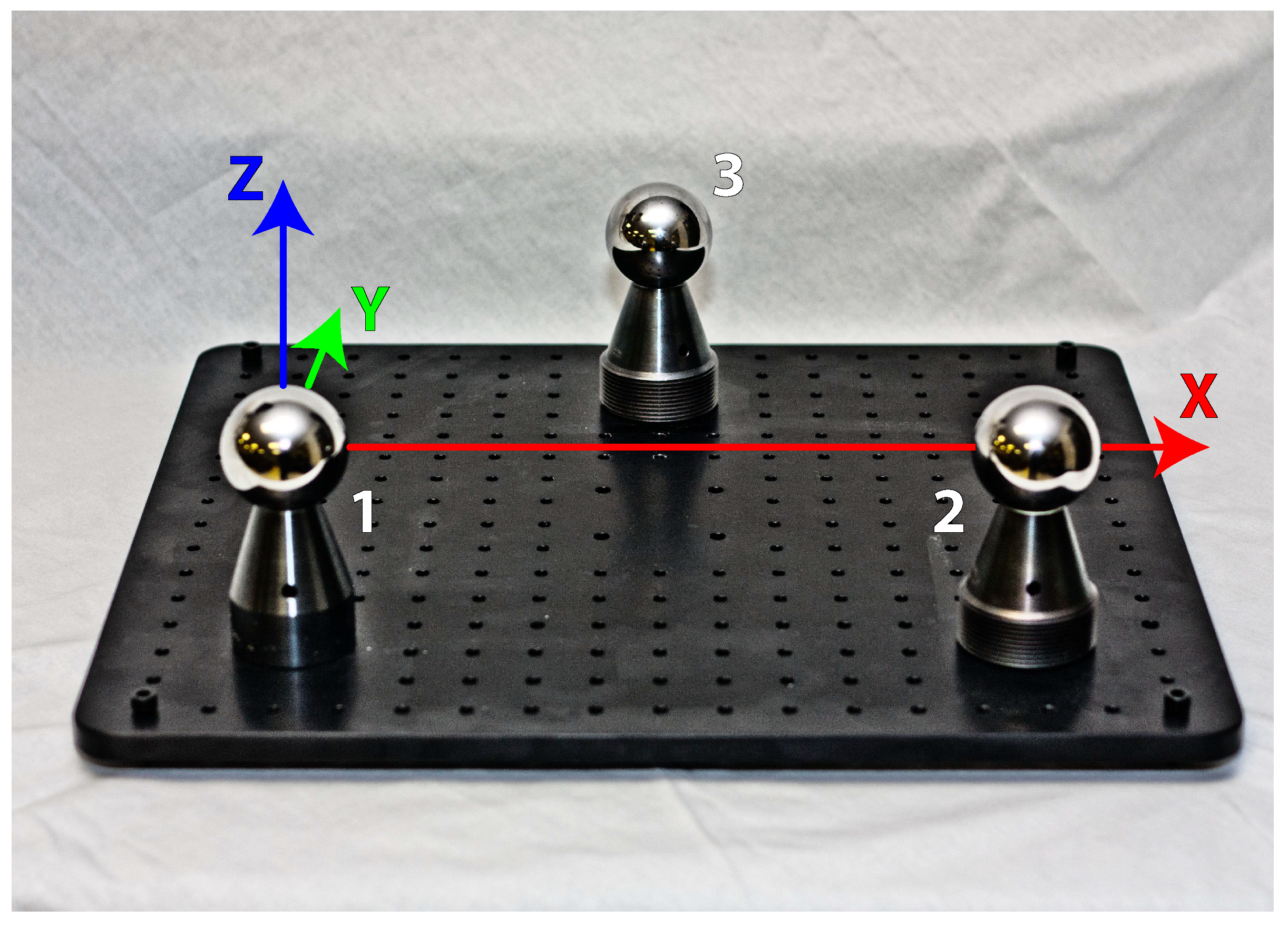
9] and the spherical constraint presented in [10], the present study uses impedance control and a calibration plate with three precision spheres to calibrate a KUKA LBR iiwa 7 R800 collaborative robot (KUKA Robotics Corporation, Augsburg, Germany). While the standard calibration process [11,12] remains the same, the use of impedance control adds an adaptable element to the approach. This adaptability comes from the fact that the absolute accuracy between the robot and the calibration tooling is not a high priority, as impedance control allows for the coupling tool to self-centre with the spheres upon contact. In such a way, workcell design is able to remain flexible without stringent accuracy requirements, and the robot is capable of self-navigating to its own calibration waypoints. Furthermore, as a secondary contribution, the automated calibration process is managed by a modern communications framework that is based on open-source tools. As such, the framework is designed specifically for flexible and scalable interconnection and information transparency requirements [8]. Finally, the performance of this strategy is further validated through a comparison with traditional laser tracker calibration.
While the concept of using geometric constraints for robot calibration is not new, the integration of impedance control to automate and improve the process has yet to be studied. One similar approach, single endpoint contact (SEC) calibration, was shown in [13] using a ball joint fixture, but manual constraint of the robot is required, reducing automation potential. As the process uses only a single fixture point, the process calibrates the robot with respect to a virtual world frame, not a physical reference frame that would be part of the application workspace, such as that presented here. Otherwise, the plane constraint method, tested in [14], constrains the tool movement to at least three planes. However, this approach requires an expensive precision touch probe and accurate plane equations that may involve mechanical characteristics (e.g., perpendicularity, flatness) of the tooling, reducing the overall simplicity and robustness of the method. Regarding the calibration of a KUKA LBR robot, the work in [15] presented a unique calibration approach using the joint torques, but only 10 points were used to validate their calibration errors. Consequently, there were too few points for a definite measure of global accuracy. In [16], an automated measuring device was presented that also uses tooling spheres. Despite this, the device itself is relatively fragile and requires Bluetooth, which may have poor performance due to the harsh electromagnetic ambient environment of industrial settings [17]. Given the current state of research, a driving motivation for this study was to develop a geometric constraint calibration process that leveraged modern robot control theory and capability while considering the current needs of industrial applications and environments.
The remainder of this article is organized as follows. In Section 2, the technical details of robot modelling and kinematics are presented, while Section 3 addresses aspects of kinematic parameter identification. Section 4 describes the methodology of the calibration processes, and Section 5 presents the validation results. Finally, Section 6 discusses the outcomes of this study and potential future work.

2. Calibration Model

The developed calibration procedure was tested with a seven-axis KUKA LBR iiwa 7 R800 robot (Figure 1). Having seven revolute joints allows this robot to have kinematic redundancy and to execute joint motions through its null space for a given Cartesian pose. The calibration model presented identifies the kinematic parameters associated with the robot and the world and tool frames. This allows for a more accurate representation of the robot application.

2.1. World and Tool Frames

The world frame ( F w ) of the application describes the origin of the Cartesian space and is the base reference for all measurements. As shown in Figure 2, this frame is represented by the right-handed coordinate system defined by the three calibration spheres. Similarly, the tool frame ( F T ; Figure 3) describes the tool centre point (TCP) of the equipped robot tool with respect to the natural flange of the robot and is located at the centre of a coupled sphere. In the present study, six degrees of freedom (three translation and three rotation) were considered for the transformation between the world frame and the robot base (located at the intersection of the first two joints). As position accuracy was the focus of the study, only translational degrees of freedom were considered for the transformation between the robot flange and the tool frame.

2.2. Tooling

The experimental tooling, shown in Figure 2 and Figure 3, was composed of a trihedral coupling (mounted eccentrically from the flange centre) and a calibration plate with 50.8 mm precision spheres. The total mass of this tooling was 1.5 kg. Both the coupling and spheres were sourced as stock components from Bal-Tec (https://www.precisionballs.com). Notably, the trihedral coupling has a strong embedded magnet (2.7 kg pull strength), which aids in mating the part to the steel sphere. Prior to the experiment, the absolute positions of the spheres (Table 1) were obtained using a Mitutoyo Bright-STRATO 7106 CMM with an uncertainty of ±2.7 µm (95% confidence level).

2.3. Kinematic Model

The KUKA LBR iiwa 7 R800 robot was modelled using modified Denavit–Hartenberg (MDH) parameters [18], describing the geometric parameters and the kinematic chain from the robot base ( F 0 ) to flange ( F 7 ). Using this convention, the forward kinematics calculation of a given set of joint angles results in a position and orientation in Cartesian space.
Given a joint angle vector:
q = [ θ 1 θ 7 ] T
Any position and orientation of the tool with respect to the world frame can be described as a series of transformations along the kinematic chain of the robot:
T T W = T 0 W T 7 0 ( q ) T T 7
where,
T 7 0 ( q ) = T 1 0 ( θ 1 ) T 2 1 ( θ 2 ) T 6 5 ( θ 6 ) T 7 6 ( θ 7 )
Each ith transformation along a link in the kinematic chain may be defined by a tuple of MDH parameters (i.e., α i 1 , a i 1 , θ i , and d i ), as detailed by the following:
T i i 1 = cos ( θ i ) sin ( θ i ) 0 a i 1 sin ( θ i ) cos ( α i 1 ) cos ( θ i ) cos ( α i 1 ) sin ( α i 1 ) sin ( α i 1 ) d i sin ( θ i ) sin ( α i 1 ) cos ( θ i ) sin ( α i 1 ) cos ( α i 1 ) cos ( α i 1 ) d i 0 0 0 1

2.4. Non-Kinematic (Stiffness) Model

Under ideal rigid body mechanics, the geometric parameters described in Section 2.3 would be sufficient for a full calibration. However, under real-world external forces (e.g., gravity), non-kinematic parameters may have negative effects on the accuracy of the robot. As described in [1,19], a simplified model of gearbox stiffness may be used to account for these sources of error. By modelling the gearbox of each joint as a linear torsional spring with stiffness k i , joint deflections due to the applied external joint torques ( τ i ) were accounted for, as given by δ θ = k τ . As the robot was studied under static conditions, only external torques due to gravity were observed.
Initial experiments demonstrated a negligible effect (but greatly increased computational time) by including the non-kinematic parameters due to joint stiffness during calibration. As the robot was gently coupled to a sphere, the structural closed-loop acted as a support against gravity. As such, these errors are not considered for the calibration process.

3. Parameter Identification

In the presented calibration, 21 kinematic errors were considered. While in theory, there are 28 kinematic error parameters, each associated with a MDH parameter, seven of these were found to be redundant and would degrade the efficiency of the applied optimization method. All considered kinematic errors may be seen in Table 2.

3.1. Non-Identifiable and Redundant Parameters

Several parameters in the robot model were not identifiable due to Cartesian and kinematic redundancies. A direct effect of these redundant parameters is two-fold. First, they increase the number of dimensions in the calibration solution space, increasing the computational requirements and complexity. Second, they reduce the ability of the optimizer to converge to an optimal solution using the change in the optimization vector as a stopping criterion.
Given that the position and orientation of the robot base were tied directly to the definition of the world frame, the first four kinematic error parameters associated with the transformation between the robot base and the first joint (i.e., α 0 , a 0 , θ 1 , and d 1 ) were excluded, as the world frame was identified separately. Additional kinematic parameters were excluded through an analysis of the rank and condition number of the robot position Jacobian [10], as shown below.
Given a robot TCP position (P) as a function of the MDH parameters,
P = x y z = f x ( α i 1 , a i 1 , θ i , d i ) f y ( α i 1 , a i 1 , θ i , d i ) f z ( α i 1 , a i 1 , θ i , d i )
the position Jacobian ( J P ) may be described as:
J P = x α i 1 x a i 1 x θ i x d i y α i 1 y a i 1 y θ i y d i z α i 1 z a i 1 z θ i z d i
where the number of columns equals the number of MDH parameters currently being considered. Following the derivation of the Jacobian, the nominal MDH values were substituted into the J P . Next, the corresponding position (x, y, z) of 29 uniformly-distributed joint configurations across the whole joint space was computed and substituted into J P , giving an augmented Jacobian ( J P ) with 87 rows. A minimum of 10 configurations were required to generate an overdetermined system, as we had 28 unknowns with three constraints per joint configuration. By defining the Jacobian around these joint configurations, we represented the relationship between an infinitesimal MDH parameter change (i.e., α , a , θ , d ) and the respective infinitesimal displacement (i.e., x , y , z ) of the TCP across the joint configuration space covered by the 29 joint positions. The rank ( r J P ) of the augmented Jacobian quantifies the number of identifiable kinematic parameters, while the condition number ( c J P ) represents the sensitivity of this relationship. The condition number is defined as the L2-norm of the Jacobian times the L2-norm of the inverse of the Jacobian (computed directly using SVD), and the calculation was implemented by the Python scientific computing package NumPy in the function numpy.linalg.cond. The non-identifiable parameters (columns of the Jacobian) were removed using Algorithm 1 to generate a more well-conditioned problem. In the present study, δ d 6 , δ a 6 , and δ θ 7 were found to be redundant. A more detailed analysis of this selection algorithm may be seen in [9,10].

3.2. Optimization and Numerical Modelling

With the identifiable parameters, an optimal set may be found that improves the accuracy of the robot. Like [6,10], distance errors between spheres were used for robot model optimization, removing the dependency (and associated errors) of the world frame from the calibration step. The relative distance fitness function ( f f i t ) for a current set of robot parameters is defined below through Equations (1) to (3) and the real sphere positions ( P s p h e r e i and P s p h e r e j ).
Algorithm 1 Redundant parameter identification
 calculate condition number of J P , c J P
 calculate rank of J P , r J P
m i n C o n d i t i o n N u m b e r c J P
c o l u m n T o R e m o v e n u l l
while r J P < number of columns in J P do
  for column i in J P do
    J * J P
   remove column i from J *
   calculate condition number of J * , c J *
   calculate rank of J * , r J *
   if r J * = = r J P then
    if c J * < m i n C o n d i t i o n N u m b e r then
      m i n C o n d i t i o n N u m b e r c J *
      c o l u m n T o R e m o v e i
    end if
   end if
  end for
  remove column c o l u m n T o R e m o v e from J P
end while
Given the absolute position of two spheres and two associated measurement configurations,
P s p h e r e = x s p h e r e y s p h e r e z s p h e r e
P T C P ( q ) = T x t w T y t w T z t w
the real distance ( D s p h e r e i , j ) between spheres i and j were found,
D s p h e r e i , j = P s p h e r e i P s p h e r e j
Next, the forward kinematic TCP distance between measured spheres i and j were found,
D T C P i , j ( m , q ) = P T C P ( m , q i ) P T C P ( m , q j )
where m represents the current set of MDH parameters. These parameters were the array of parameters to be optimized during calibration.
Finally, the relative fitness was calculated for all given combinations,
f f i t ( m , q ) = ( D s p h e r e i , j D T C P i , j ( m , q ) ) 2
where i and j correspond to the ith and jth measured configuration coupled with a sphere.
The Nelder–Mead method (equivalent to fminsearch in MATLAB) [20] was used for optimization with the above fitness function and initialized with the nominal robot model. This method is robust to noise and works well with non-locally smooth data, such as discrete and noisy measurement data. At each solver iteration, the forward kinematic relative distance errors were evaluated for a given set of robot parameters. The numerical methods and kinematic modelling were implemented using Pybotics (https://github.com/nnadeau/pybotics), allowing multicore processing and a direct interface to the optimization methods implemented by the SciPy Python package.

4. Methodology

Three primary components formed the basis of this study: communication, measurement, and calibration. First, a modern communications architecture was developed to transmit data and command packets between an external PC controller, the KUKA LBR iiwa robot, and a FARO ION laser tracker. Next, with a common communications and data processing framework, impedance control and tradition laser measurement and calibration processes were developed.

4.1. Communication

A calibration framework viable for adaptability and scalability requires the use of modern data processing protocols. As such, the calibration communications architecture was designed to satisfy Levels 1–3 of the cyber-physical system (CPS) requirements, as defined in [21]. Plug and play (PnP) decentralized services allow for messaging patterns where data can be integrated with various systems in a smart factory network. From this interconnection, meaningful information can be inferred from the data, such as robot calibration quality and workcell health. Over the lifecycle of the robotic system, machine performance and historical data can be used to predict future behaviour.
Given these criteria, protocol buffers (https://developers.google.com/protocol-buffers/) were selected as the mechanism for serialized structured data (i.e., packets), and gRPC (https://grpc.io/) was selected as the transmission mechanism. Figure 4 illustrates the control and data flow of this architecture.
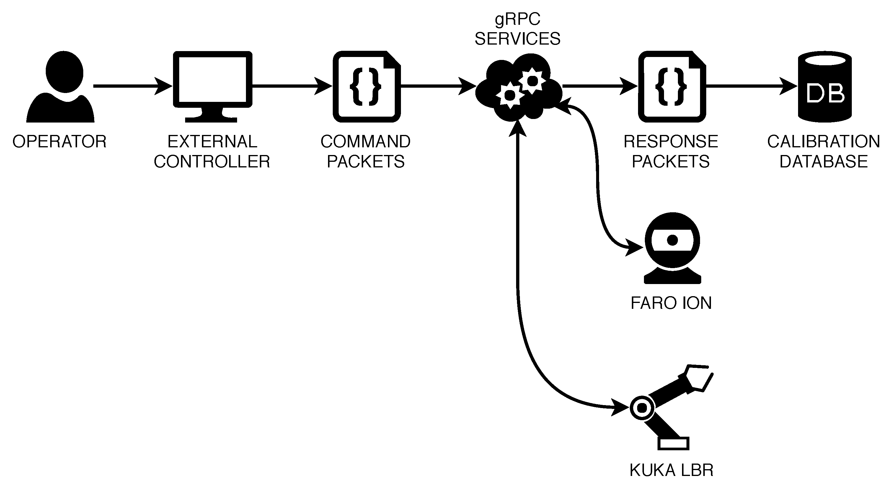
Specifically, the external controller that manages the automation of the entire calibration process uses protocol buffer packets and gRPC to communicate across the network with the robotic devices and calibration database. This distributed computing architecture is based on remote procedure call (RPC), a type of a client-server model. With the RPC protocol, a program can request a service or function from another program without having to understand the network layout, such as the relative location of the two programs (i.e., on the same computer or on different devices). The requesting program is a client (e.g., external controller), and the service providing program is the server (e.g., FARO ION controller, KUKA LBR controller, calibration database). In the presented architecture (Figure 4), the command packets tell the robot and laser tracker where, when, and how to move. Following the movement command, these devices reply with a response packet that contains the necessary data for calibration (e.g., joint values, Cartesian position). These responses are collected by the external controller and are stored in a database.
The primary advantage of this model is the ability to develop a microservices-style architecture where device control (e.g., robot control, laser tracker control) and data processing become abstract services from the perspective of the external PC controller. A second advantage is the programming language and platform neutral nature of the chosen mechanisms, allowing for straightforward integration with the robot and laser tracker firmware and APIs.

4.2. Sphere Measurement and Calibration

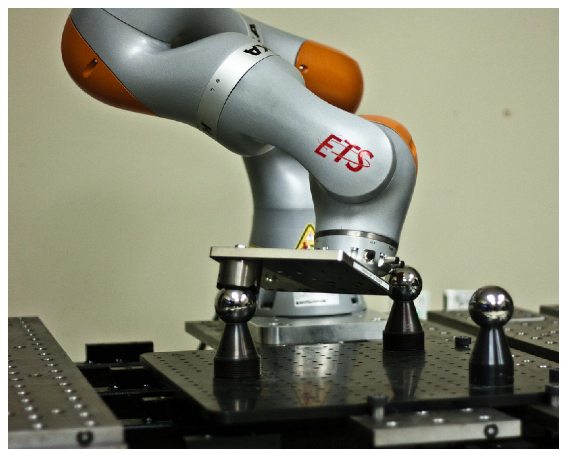
The impedance control measurement phase focuses on the collection of data using controlled coupling events. First, whether through manual jogging, offline programming, or hand-guiding, the general location of the three spheres is recorded. In the case of this study, as the KUKA LBR robot is a collaborative robot, these waypoints were taught by quickly hand-guiding the robot to each sphere.
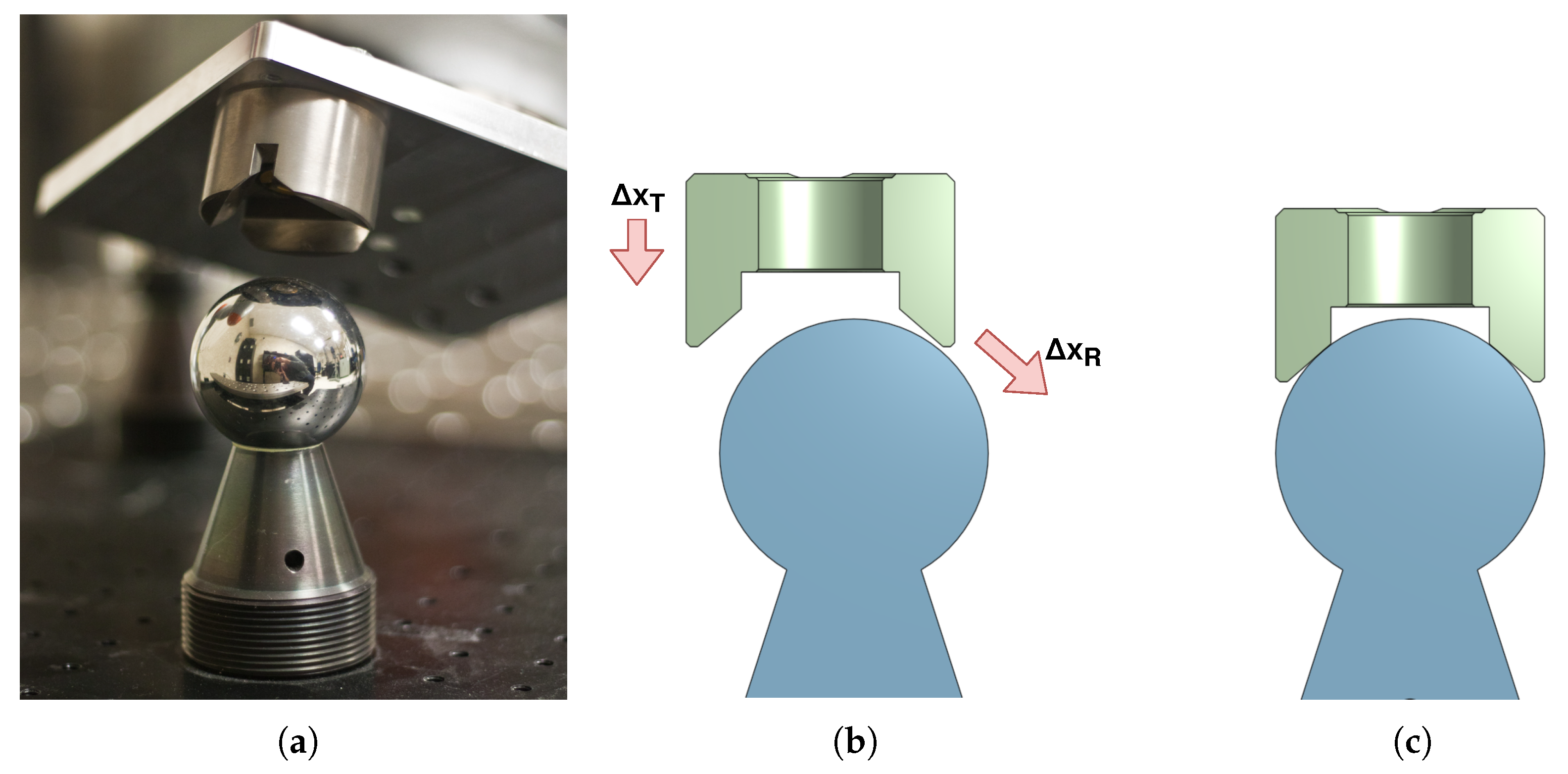
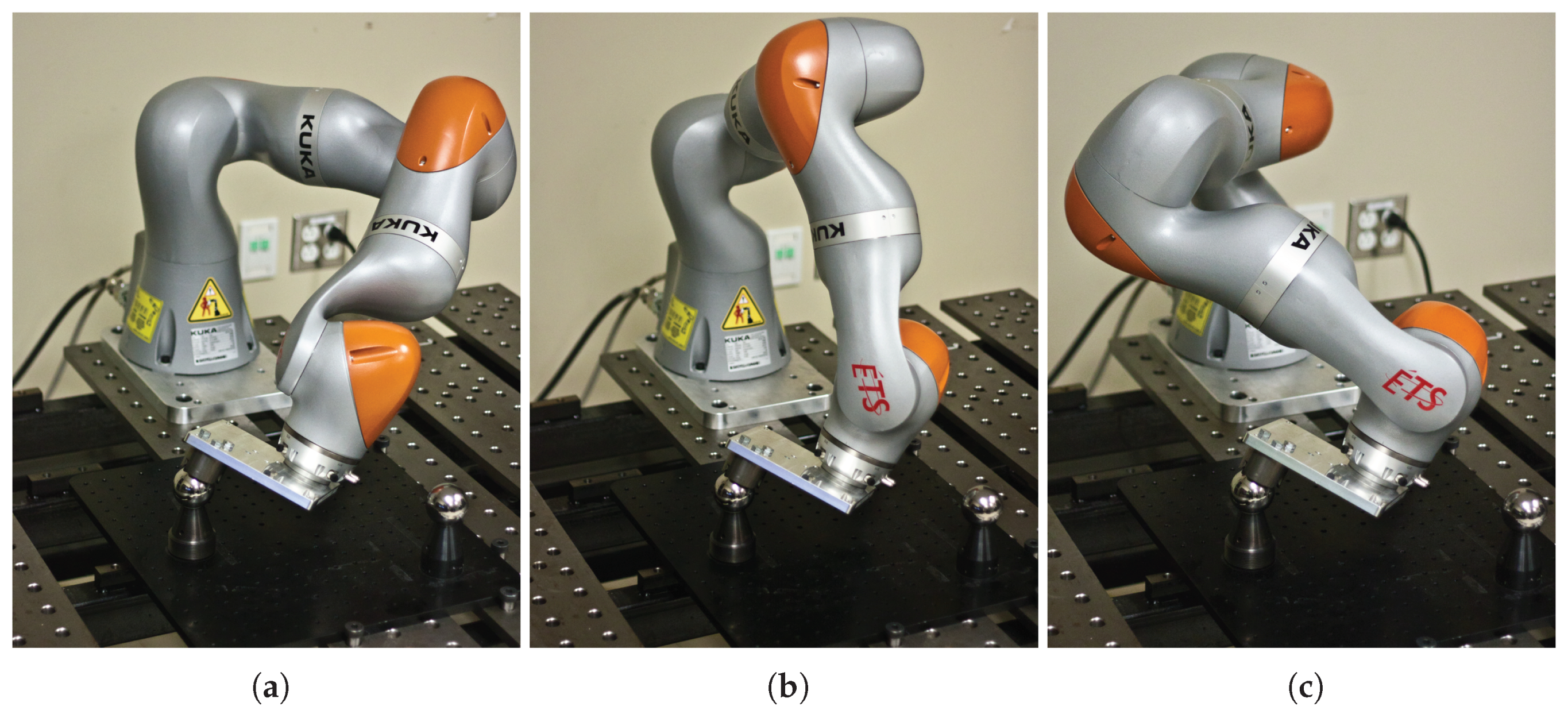
Next, the automated calibration process begins and is outlined in Algorithm 2. For each sphere, the automated process followed a simple series of steps: contact, record, and decouple. As the robot was under impedance control with a kinematic coupling and magnet, the accuracy of the saved sphere waypoints was not a high priority, and the robot will self-centre upon contact (Figure 5), as illustrated in Figure 6.
Algorithm 2 Sphere calibration process. All motions are under impedance control. The approachFrame may be programmed offline or taught using hand-guiding. The homeFrame represents a safe starting point for robot motions
 robot.move( h o m e F r a m e )
for sphere i in [1,2,3] do
  // move above sphere i
  robot.move( a p p r o a c h F r a m e )
  // prepare for sphere contact
  robot.setXStiffness(50)    // N/m
  robot.setYStiffness(50)    // N/m
  robot.setZStiffness(100)    // N/m
  robot.setForceTrigger(7.5)    // N
  // contact sphere
  while !isContact do
   robot.moveWithVelocity(25)    // mm/s
  end while
  // allow the strong magnet to couple fully
  robot.setXYZStiffness(5)    // N/m
  robot.holdPosition(5)    // s
  // receive poses from external controller and record joints
  while n e x t P o s e ← getPose() ! = n u l l do
   // move to pose
   robot.setXYZStiffness(20)    // N/m
   robot.move( n e x t P o s e )
   // record joint data over a period of time
   robot.setXYZStiffness(5)    // N/m
   robot.startRecording()
   robot.holdPosition(1)    // s
   robot.stopRecording()
   // transmit joint data to database
    j o i n t D a t a ← robot.getRecording()
   uploadData( j o i n t D a t a )
  end while
  // decouple from sphere
  robot.decouple()
  robot.move( h o m e F r a m e )
end for
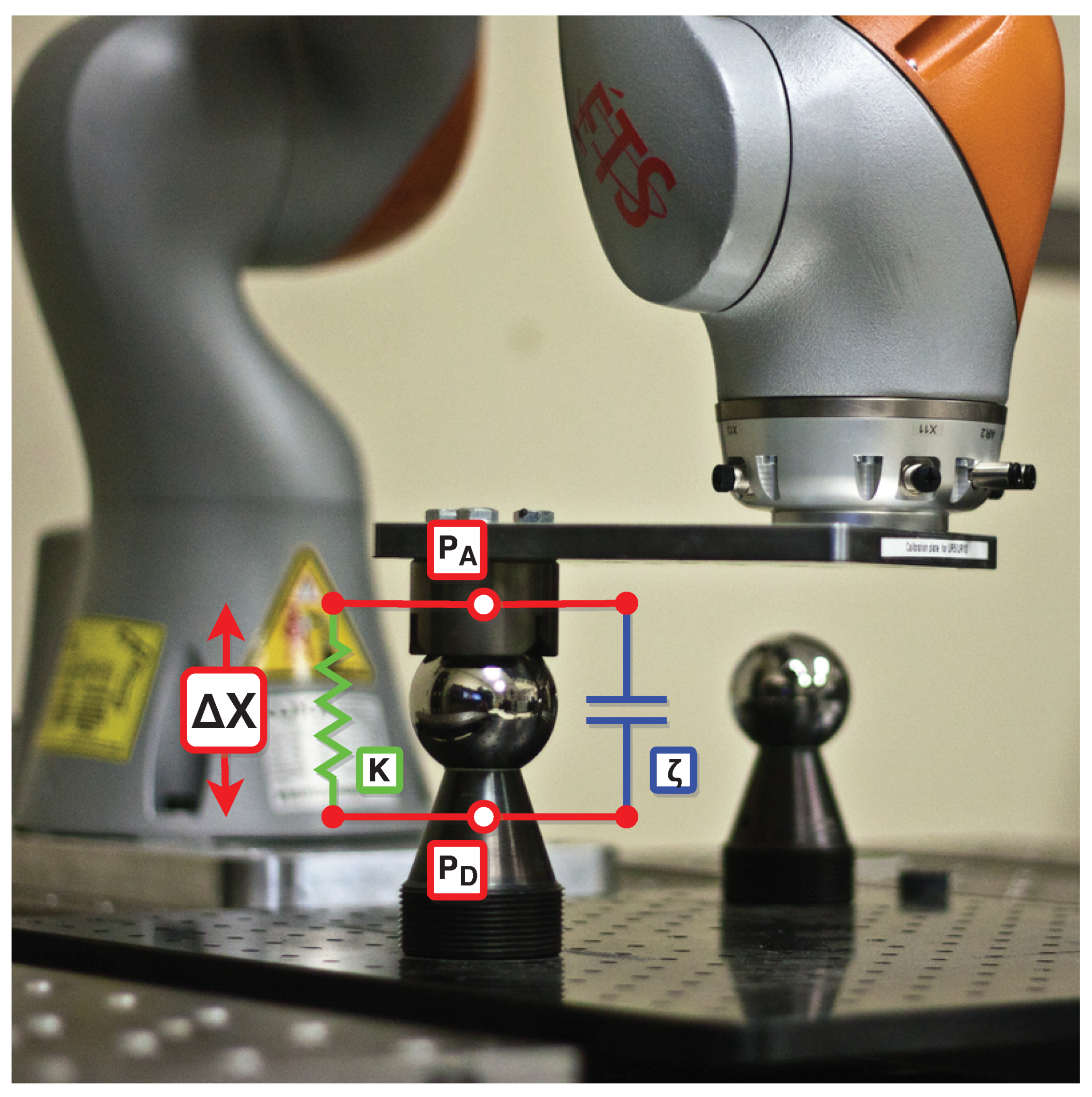
The control architecture exploited the built-in real-time impedance control of the LBR robot as the base control strategy (KUKA Sunrise.OS v1.10). The basic model was a virtual spring-damper system with configurable values for stiffness and damping, allowing the KUKA LBR to be highly sensitive and compliant (Figure 7). As outlined in Algorithm 2, the axis stiffness values, K, were independently updated throughout different phases of the measurement process. The axis damping coefficients (Lehr’s damping ratio) remained constant and were set to ζ = 0.7.
Subsequently, the robot will iterate through a series of coupled poses commanded by the external controller. At each pose, the robot held a position under impedance control, allowing the strong magnet to maintain proper coupling. The robot controller then logged the robot joint angles and torque values at a rate of 1000 Hz for 1 s, allowing for mechanical stabilization. These data were transmitted back to the external controller and uploaded to a database for future processing. During the calibration process, the mean joint values of this logging process were used. Further mechanical stability analysis demonstrated that even over a period of 30 s, the maximum deviations from the mean values were negligible for the joint angles. Following the completion of the recording phase, the robot decoupled itself from the sphere and repeated the process on the next sphere.
All calibration poses were defined as relative frames with respect the robot base orientation and centred at the sphere. Thus, for each frame, the position of the TCP remained constant, but the tool coupling rotated about the sphere. The frames were generated from a distribution of −20° to 20° in 10 ° steps about all three rotational axes. As the KUKA LBR is a redundant robot with seven axes, each pose was further expanded by altering the redundant α angle (i.e., the angle formed between the elbow of the robot and the vertical base axis) through the same angular distribution (Figure 8). A total of 625 poses was generated and recorded on each sphere.
Using the data collected and the optimization algorithms and models presented in Section 3.2, the robotic system was calibrated using relative distance errors. As 625 poses per sphere would result in 1,756,875 combination pairs, the dataset was reduced to 100 pairs per sphere (44,850 combinations) through random selection. Moreover, mini-batch optimization with a batch size of 32 was used for computational efficiency [22].

4.3. Laser Measurement and Calibration

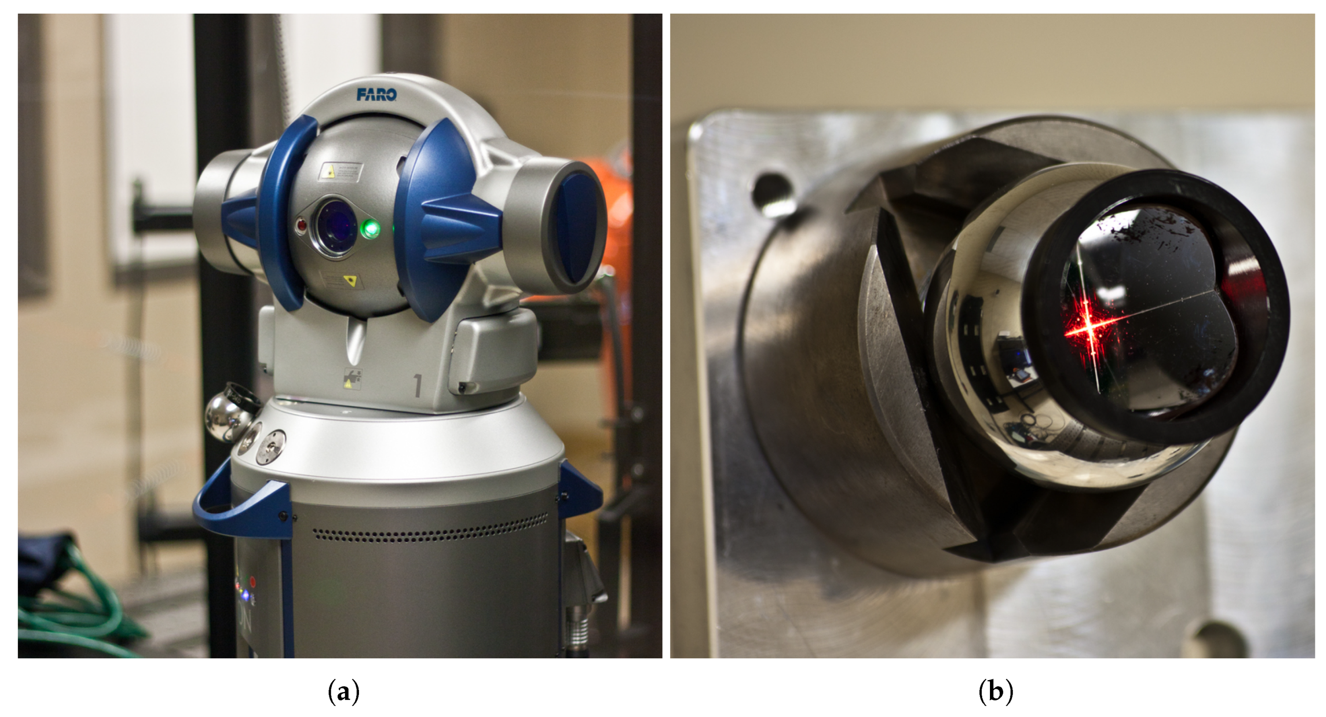
To validate the quality of the impedance control calibration method properly, traditional calibration with a FARO ION laser tracker (uncertainty of ±49 µm) and spherically-mounted retro-reflectors (SMR) was performed (Figure 9). Following the procedure outlined in [1], 284 uniformly-distributed joint configurations were recorded within the workspace of the robot for calibration (Table 3). An additional dataset of 125 configurations was recorded for validation (Table 4). The 3D distribution of these points may be seen in Figure 10.
To calibrate the robot base frame and the tool frame, 150 and 153 additional measurements were recorded, respectively. The base frame measurements were generated by independently rotating only Joints 1 and 2 to produce two 3D arc trajectories whose intersection gave the location of the base frame. Similarly, the tool frame measurements were generated by independently rotating only Joints 5, 6, and 7. The independently-measured base and tool frames were used not only during the laser calibration, but also during validation, acting as control variables for the model comparison. As a result, the calibrated robot models were isolated for comparison.
Like Section 3.2, the identified kinematic parameters were independently optimized using absolute accuracy errors and the Nelder–Mead method. For absolute position optimization, using Equations (1) to (3) and (8), the absolute position error ( E a b s i ( q ) ) per measurement configuration is described as follows:
P m e a s u r e = x m e a s u r e y m e a s u r e z m e a s u r e
E a b s i ( q ) = | ( P m e a s u r e i P T C P ( q ) ) |
where i is the ith measured configuration measured by the laser tracker.

5. Results

Following impedance control and traditional calibrations, the absolute accuracy of the calibrated models was compared against the nominal model using the 125 measures mentioned in Section 4.3 and Equation (13). Error distributions between the nominal model and the calibrated models are visualized in Figure 11 and Figure 12. As shown in Figure 11, both calibration methods offered significant accuracy improvements over the nominal model. Figure 12 offers a more detailed comparison between traditional laser tracker calibration and the impedance control method. Error statistics of all the models are summarized in Table 5. The calibrated kinematic model of the KUKA LBR iiwa 7 using impedance control may be seen in Table 6.

6. Discussion

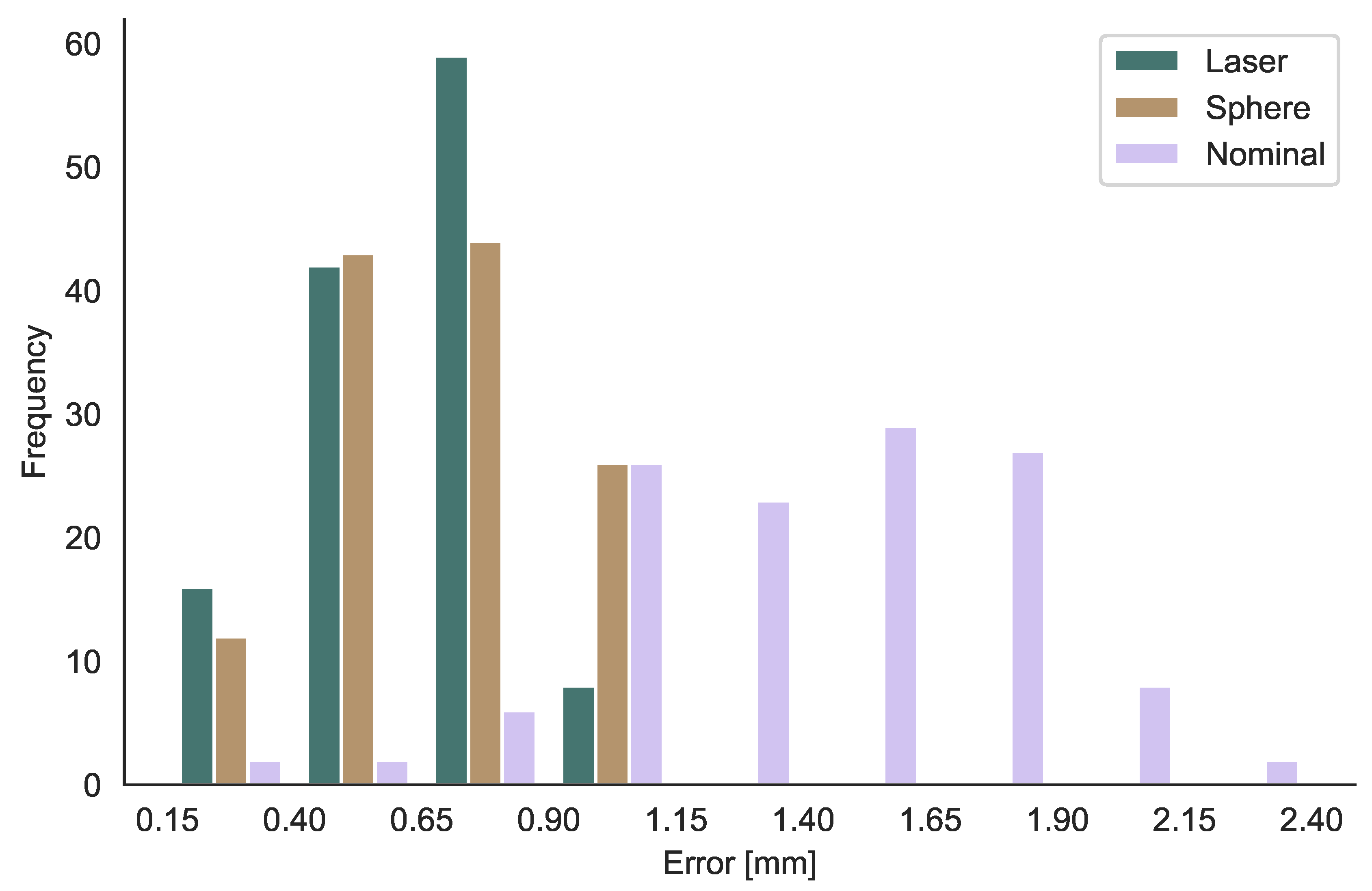
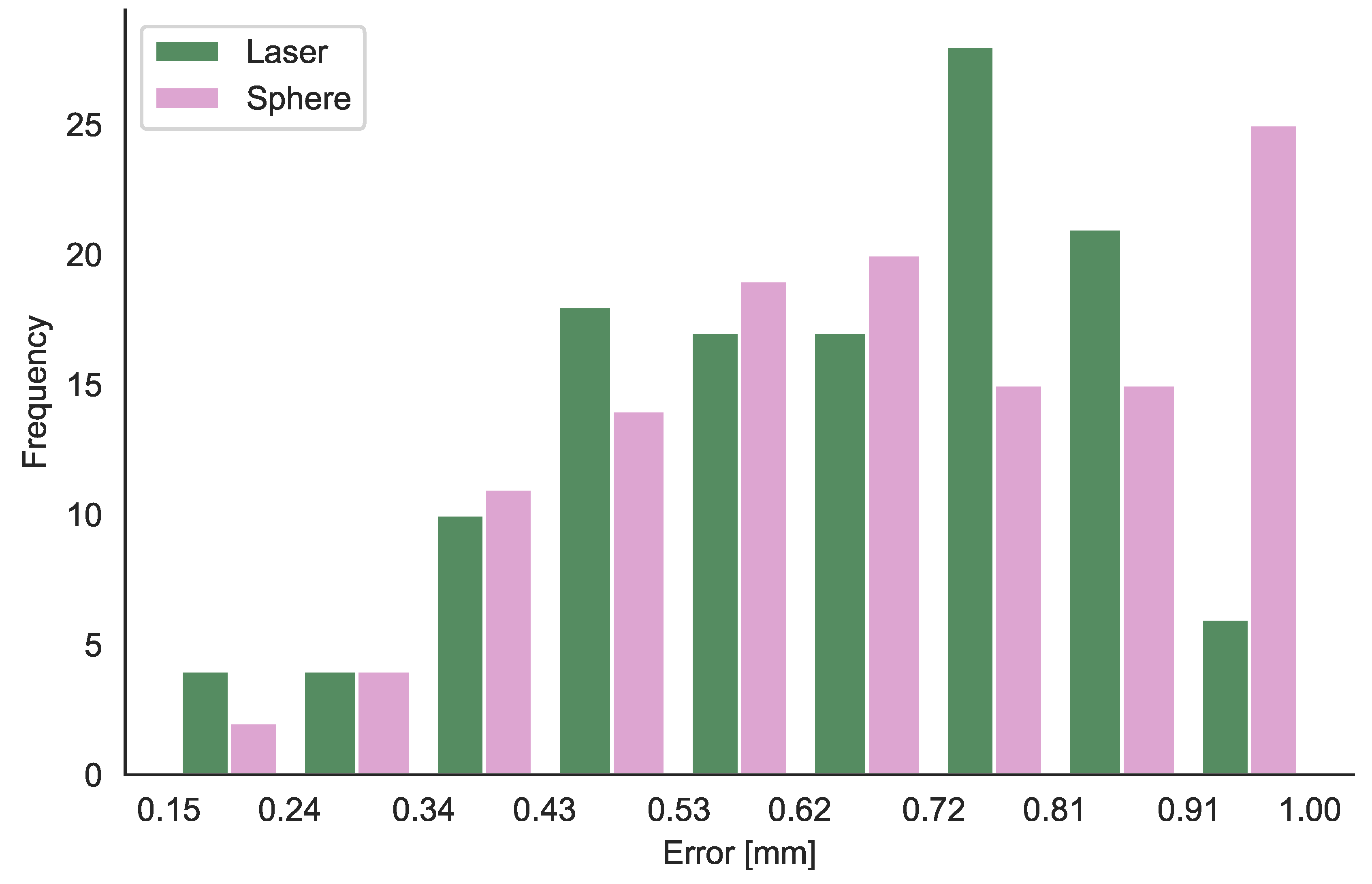
This paper presented an impedance control approach to robot calibration and compared the novel method to traditional calibration with a laser tracker. The calibration tooling has the advantage of being low-cost, robust, and simple to use, with little start-up time required. As shown through absolute accuracy validation, this calibration approach can improve the accuracy of a KUKA LBR iiwa 7 R800 collaborative robot upwards of 58.4% to a maximum error of 0.990 mm when compared to the nominal model.
It should be noted that the sheer simplicity of the tooling used in this study makes for an interesting comparison to typical calibration equipment, especially when considering the cost difference. While the traditional laser tracker calibration was capable of reducing the maximum error to 0.932 mm, the tooling presented in this study cost a total of approximately $2000 USD, while a laser tracker costs in the range of $100.000 USD. Furthermore, the robot modelling software (Pybotics; https://github.com/nnadeau/pybotics) and the communication packages are open-source and available for both industrial and academic use. It thus becomes an engineering economics issue in order to justify a $98.000 USD cost difference for an additional percentage point of improvement.
With respect to previous studies, the present study advances the literature in several distinct ways. First, while the nominal errors of the KUKA LBR agreed with [15], the presented calibration approach has been validated with 12.5-times the number of validation points, offering a more robust and confident examination of calibration quality. Compared to the self-calibration approach presented in [16], while the resulting accuracies due to the methods cannot be directly compared (two different robots), the difference between their method and the (same) laser tracker was relatively equivalent. Yet, the method presented here is even less expensive and more durable for industrial environments. While often undervalued, durability and robustness are key considerations, as repairs and workcell downtime can be expensive.
Although this study used a redundant robot, this method can easily be applied to less sophisticated robots with no major differences in procedure. While redundant motion allows many joint configurations for a single Cartesian pose, the results of this process with a non-redundant robot will produce a dataset without redundant configurations. Simply put, redundant motion produces more joint configurations with less tool movement.
From a manufacturing and operations perspective, the authors of [23,24] described a set of guidelines for a resilient manufacturing system (RMS), whereby the system is fault tolerant and capable of recovering from failure. In the case of the presented calibration methodology, failure may occur during any of the steps outlined in Section 4.2. During the contact, coupling, and motion steps, force limits are set to prevent damage to the tooling, and the recovery process is to simply decouple, move away, and restart the coupling procedure. Returning to a known stable position is not required and slows the overall process. During the recording phase, the system follows redundancy guidelines and records more poses than necessary for calibration optimization. Further reliability can be achieved through the robot communication and control framework described in Section 4.1, where data collection can be used to develop continuous improvement initiatives. This communication framework integration follows Guidelines II–IV presented in [23]. In an ideal integration, the presented calibration tooling would become part of the robot workcell, allowing the robot to self-validate and calibrate. As noted in [21], with a connected fleet of machines and an awareness of machine condition, predictive maintenance and workload balancing become possible and maximize machine performance and organization transparency.

Author Contributions

Conceptualization, N.A.N. and A.J.; data curation, N.A.N.; formal analysis, N.A.N.; funding acquisition, I.A.B.; investigation, N.A.N.; methodology, N.A.N.; software, N.A.N.; supervision, I.A.B.; validation, N.A.N.; visualization, N.A.N.; writing, original draft, N.A.N.; writing, review and editing, N.A.N., I.A.B., and A.J.

Funding

This work was supported by the Canada Research Chair on Precision Robotics.

Conflicts of Interest

The authors declare no conflict of interest.

References

  1. Nubiola, A.; Bonev, I.A. Absolute calibration of an ABB IRB 1600 robot using a laser tracker. Robot. Comput.-Integr. Manuf. 2013, 29, 236–245. [Google Scholar] [CrossRef]
  2. Zhao, L.; Joubair, A.; Bigras, P.; Bonev, I.A. Metrological evaluation of a novel medical robot and its kinematic calibration. Int. J. Adv. Robot. Syst. 2015, 12, 126. [Google Scholar] [CrossRef]
  3. Nubiola, A.; Slamani, M.; Joubair, A.; Bonev, I.A. Comparison of two calibration methods for a small industrial robot based on an optical CMM and a laser tracker. Robotica 2014, 32, 447–466. [Google Scholar] [CrossRef]
  4. Svaco, M.; Sekoranja, B.; Suligoj, F.; Jerbic, B. Calibration of an Industrial Robot Using a Stereo Vision System. Procedia Eng. 2013, 69, 459–463. [Google Scholar] [CrossRef]
  5. Joubair, A.; Slamani, M.; Bonev, I.A. A novel XY-Theta precision table and a geometric procedure for its kinematic calibration. Robot. Comput.-Integr. Manuf. 2012, 28, 57–65. [Google Scholar] [CrossRef]
  6. Gaudreault, M.; Joubair, A.; Bonev, I.A. Local and closed-loop calibration of an industrial serial robot using a new low-cost 3D measuring device. In Proceedings of the IEEE International Conference on Robotics and Automation, Stockholm, Sweden, 16–21 May 2016; pp. 4312–4319. [Google Scholar] [CrossRef]
  7. Borm, J.H.; Menq, C.H. Determination of optimal measurement configurations for robot calibration based on observability measure. Int. J. Robot. Res. 1991, 10, 51–63. [Google Scholar] [CrossRef]
  8. Lee, J.; Bagheri, B.; Kao, H.A. A cyber-physical systems architecture for industry 4.0-based manufacturing systems. Manuf. Lett. 2015, 3, 18–23. [Google Scholar] [CrossRef]
  9. Joubair, A.; Slamani, M.; Bonev, I.A. Kinematic calibration of a five-bar planar parallel robot using all working modes. Robot. Comput.-Integr. Manuf. 2013, 29, 15–25. [Google Scholar] [CrossRef]
  10. Joubair, A.; Bonev, I.A. Kinematic calibration of a six-axis serial robot using distance and sphere constraints. Int. J. Adv. Manuf. Technol. 2015, 77, 515–523. [Google Scholar] [CrossRef]
  11. Elatta, A.Y.; Gen, L.P.; Zhi, F.L.; Yu, D.; Fei, L. An Overview of Robot Calibration. Inf. Technol. 2004, 3, 74–78. [Google Scholar]
  12. Mooring, B.W.; Roth, Z.S.; Driels, M.R. Fundamentals of Manipulator Calibration; Wiley: New York, NY, USA, 1991. [Google Scholar]
  13. Meggiolaro, M.; Scriffignano, G.; Dubowsky, S. Manipulator calibration using a single endpoint contact constraint. In Proceedings of the 26th Biennial Mechanisms and Robotics Conference of the 2000 ASME Design Engineering Technical Conferences, Baltimore, MD, USA, 10–14 September 2000; pp. 1–9. [Google Scholar]
  14. Joubair, A.; Bonev, I.A. Non-kinematic calibration of a six-axis serial robot using planar constraints. Precis. Eng. 2015, 40, 325–333. [Google Scholar] [CrossRef]
  15. Besset, P.; Olabi, A.; Gibaru, O. Advanced calibration applied to a collaborative robot. In Proceedings of the 2016 IEEE International Power Electronics and Motion Control Conference (PEMC), Varna, Bulgaria, 25–28 September 2016; pp. 662–667. [Google Scholar]
  16. Gaudreault, M.; Joubair, A.; Bonev, I. Self-calibration of an industrial robot using a novel affordable 3D measuring device. Sensors 2018, 18, 3380. [Google Scholar] [CrossRef] [PubMed]
  17. Neelakanta, P.S.; Dighe, H. Robust factory wireless communications: A performance appraisal of the Bluetooth/spl trade/and the ZigBee/spl trade/colocated on an industrial floor. In Proceedings of the 29th Annual Conference of the IEEE Industrial Electronics Society (IECON’03), Roanoke, VA, USA, 2–6 November 2003; Volume 3, pp. 2381–2386. [Google Scholar]
  18. Craig, J.J. Introduction to Robotics Mechanics and Control, 3rd ed.; Pearson Education International: London, UK, 2005. [Google Scholar]
  19. Warnecke, H.; Week, M.; Brodbeck, B.; Engel, G. Assessment of Industrial Robots. CIRP Ann. Manuf. Technol. 1980, 29, 391–396. [Google Scholar] [CrossRef]
  20. Nelder, J.A.; Mead, R. A simplex method for function minimization. Comput. J. 1965, 7, 308–313. [Google Scholar] [CrossRef]
  21. Lee, J.; Kao, H.A.; Yang, S. Service innovation and smart analytics for industry 4.0 and big data environment. Procedia Cirp 2014, 16, 3–8. [Google Scholar] [CrossRef]
  22. Bengio, Y. Practical recommendations for gradient-based training of deep architectures. arXiv 2012, arXiv:1206.5533. [Google Scholar]
  23. Zhang, W.; Van Luttervelt, C. Toward a resilient manufacturing system. CIRP Ann. 2011, 60, 469–472. [Google Scholar] [CrossRef]
  24. Zhang, T.; Zhang, W.; Gupta, M. Resilient Robots: Concept, Review, and Future Directions. Robotics 2017, 6, 22. [Google Scholar] [CrossRef]
Figure 1. Impedance controlled calibration of a KUKA LBR iiwa 7.
Robotics 08 00033 g001
Figure 2. Calibration plate with three 50.8 mm precision spheres. The origin of the world frame is located at the centre of Sphere 1. The x-axis is defined by the centres of Spheres 1 and 2. The x y -plane is defined by the centres of the three spheres.
Robotics 08 00033 g002
Figure 3. Robot calibration tool with trihedral kinematic coupling. For both the flange ( F 7 ) and tool ( F T ) frames, the x y -plane is parallel to the plate.
Robotics 08 00033 g003
Figure 4. Calibration communications framework. Protocol buffers were selected as the mechanism for serialized structured data (i.e., packets). gRPC was selected as the transmission mechanism. During the measurement phase, collected data are uploaded to a database for future processing.
Robotics 08 00033 g004
Figure 5. Recorded force data during the sphere contact event. The robot controller logs the Cartesian forces applied to the tool frame at a rate of 1000 Hz. As described in Algorithm 2, the kinematic coupling event is triggered by a 7.5 N force condition.
Robotics 08 00033 g005
Figure 6. Self-centring of the kinematic coupling under impedance control. (a) The combination of the kinematic coupling, a strong magnet, and impedance control allows for a lower accuracy of the saved sphere waypoints. (b) Upon contact, a commanded tool motion, Δ x T , will produce a resulting motion, Δ x R , that centres the nest onto the sphere (c).
Robotics 08 00033 g006
Figure 7. The built-in real-time impedance control of the KUKA LBR iiwa robot (LBR). The model is a virtual spring-damper system with configurable values for stiffness (K) and damping ( ζ ), allowing the KUKA LBR to be highly sensitive and compliant. The resulting interaction forces are calculated from the displacement ( Δ X ) between the desired position ( P D ) and the actual position ( P A ) in each Cartesian axis.
Robotics 08 00033 g007
Figure 8. Expansion of coupled poses through redundant joint configurations. All three pictured configurations represent the same Cartesian pose. The KUKA LBR is a redundant robot with seven axes, and a non-singular pose has infinite joint configurations. The redundant α angle parameter is defined as the angle formed between the elbow of the robot and the vertical base axis. (a) Robot pose with the redundant α angle parameter set to −20°. (b) Robot pose with the redundant α angle parameter set to 0°. (c) Robot pose with the redundant α angle parameter set to 20°.
Robotics 08 00033 g008
Figure 9. Traditional laser tracker calibration equipment. (a) A FARO ION laser tracker (uncertainty of ±49 µm). (b) Spherically-mounted retro-reflectors (SMR) mounted to the same tooling described in Section 2.2.
Robotics 08 00033 g009
Figure 10. 3D distribution of calibration and validation points. Two hundred eighty four configurations were used for laser calibration. One hundred twenty five configurations were used for laser validation.
Robotics 08 00033 g010
Figure 11. Histogram of validation errors comparing the nominal and calibrated models.
Robotics 08 00033 g011
Figure 12. Histogram of validation errors comparing the calibrated models.
Robotics 08 00033 g012
Table 1. Absolute positions of the three calibration spheres with respect to the world frame.
SphereX (mm)Y (mm)Z (mm)
1000
2300.00900
3150.049260.0510
Table 2. Considered kinematic parameters for the calibration and validation process. The redundant parameters are denoted with an asterisk (*).
iαi−1ai−1θidi
(rad)(mm)(rad)(mm)
10*0* θ 1 *0*
2 π 2 + δ α 1 δ a 1 θ 2 + δ θ 2 δ d 2
3 π 2 + δ α 2 δ a 2 θ 3 + δ θ 3 400 + δ d 3
4 π 2 + δ α 3 δ a 3 θ 4 + δ θ 4 δ d 4
5 π 2 + δ α 4 δ a 4 θ 5 + δ θ 5 400 + δ d 5
6 π 2 + δ α 5 δ a 5 θ 6 + δ θ 6 0*
7 π 2 + δ α 6 0* θ 7 * 126 + δ d 7
Table 3. Statistics of the 284 configurations used for laser calibration.
mean (mm)std (mm)min (mm)max (mm)
x525.872160.031−7.304947.042
y−69.712220.397−560.339452.969
z650.021186.840198.3221197.046
Table 4. Statistics of the 125 configurations used for laser validation.
mean (mm)std (mm)min (mm)max (mm)
x501.986211.902−24.214995.460
y−7.856252.262−578.336523.221
z750.930227.457137.1781135.052
Table 5. Summary of validation errors between the nominal KUKA LBR kinematic model, sphere calibration with impedance control, and traditional laser tracker calibration.
mean (mm)std (mm)min (mm)max (mm)
Laser0.6450.1920.1680.932
Sphere0.6770.2060.2250.990
Nominal1.4030.3920.3252.381
Table 6. Calibrated kinematic model of the KUKA LBR iiwa 7 using the presented impedance control approach.
iαaθd
00.0000000.0000000.000000340.000000
1−1.5707590.0000610.0000620.000062
21.5715750.000056−0.000490400.574635
31.5698420.0000610.0000610.000063
4−1.5706230.0000620.000059400.629881
5−1.5714510.0000620.0000610.000000
61.5711360.0000000.000000125.505736

