Numerical and Experimental Validation of the Prototype of a Bio-Inspired Piping Inspection Robot


Abstract
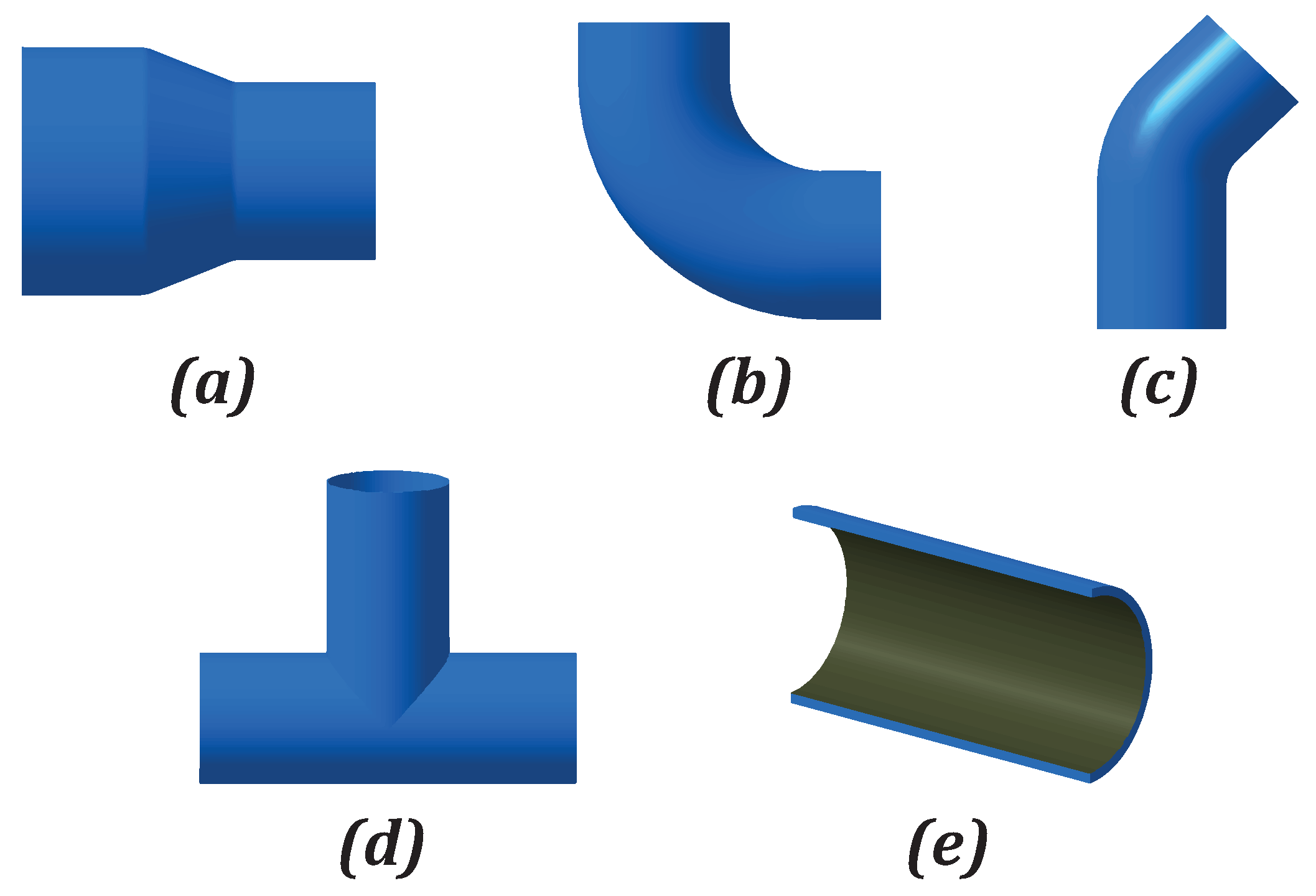
:1. Introduction
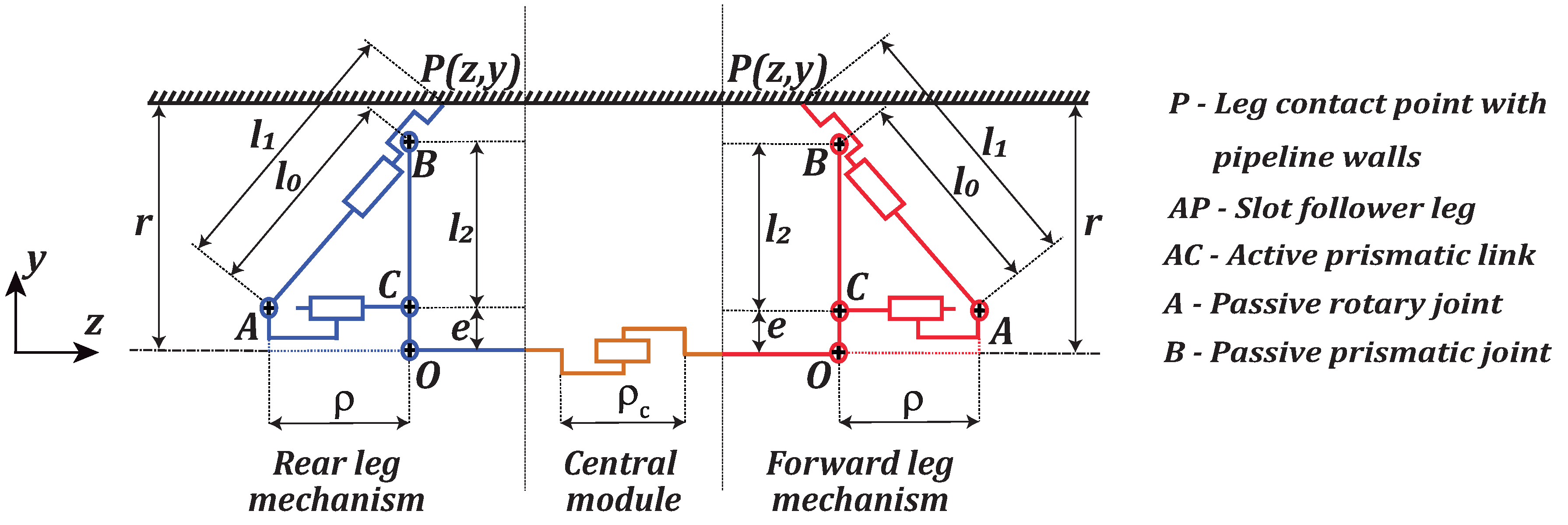
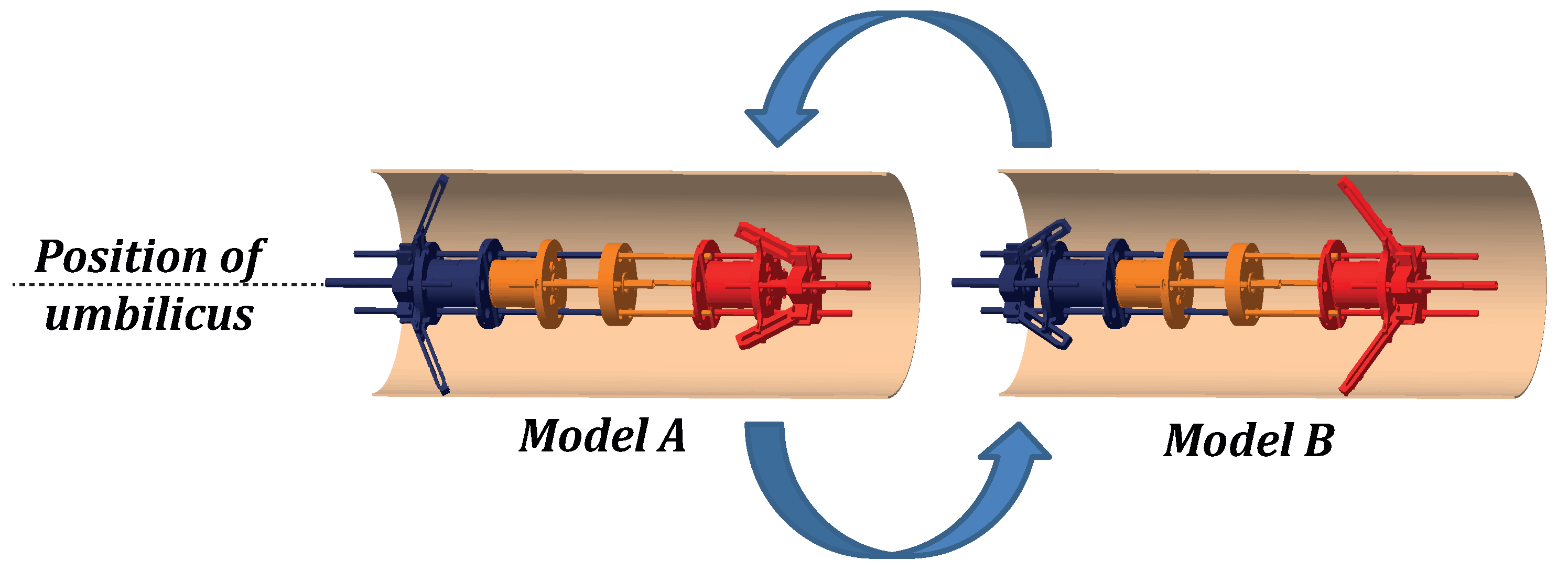
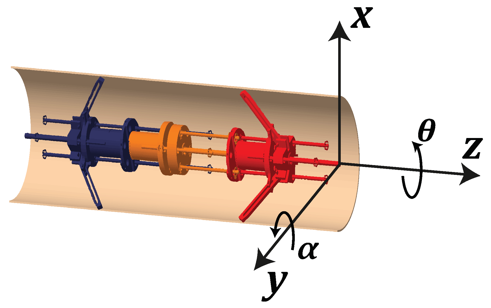
2. Locomotion Principle and Kinematic Equations of the Robot
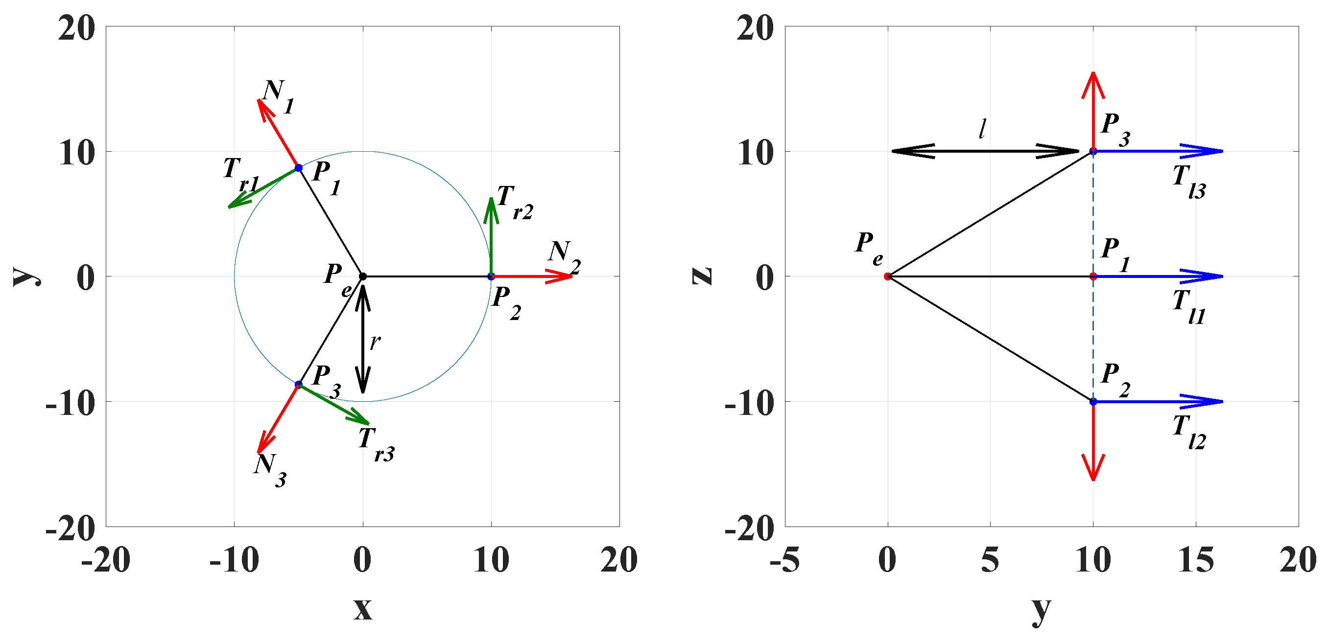
3. Static Force Analysis on the Robot
- —Normal Force
- —Tangential longitudinal Force
- —Tangential radial Force
3.1. Results of Static Force Analysis
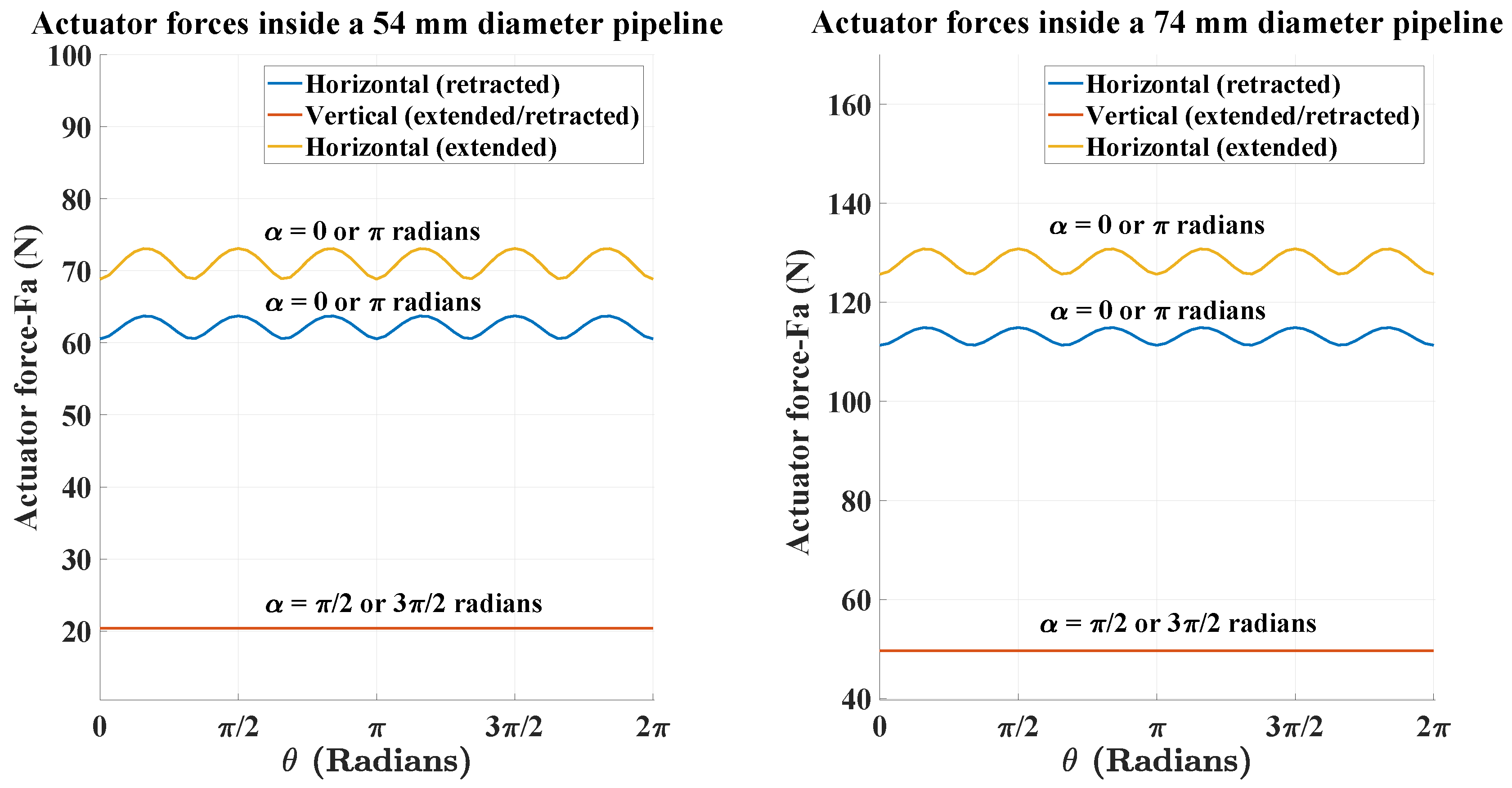
Forces Inside Horizontal and Vertical Orientations of Pipeline
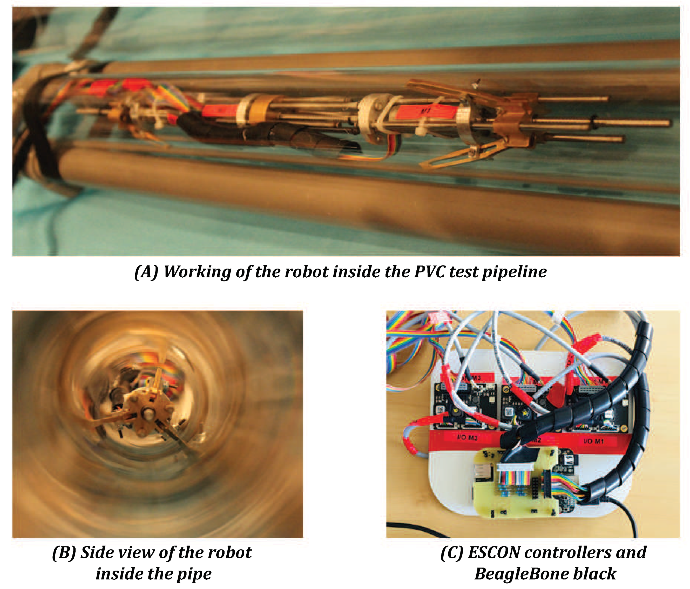
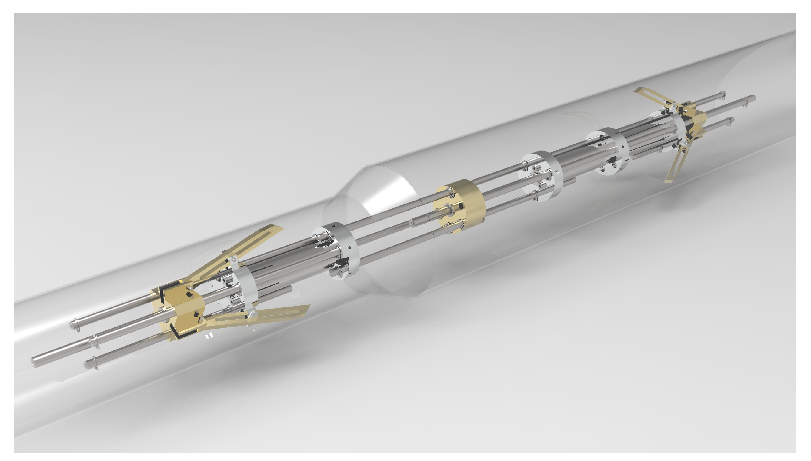
4. Experimental Validation of the Prototype
| Algorithm 1 Forward sequence force algorithm. |
|
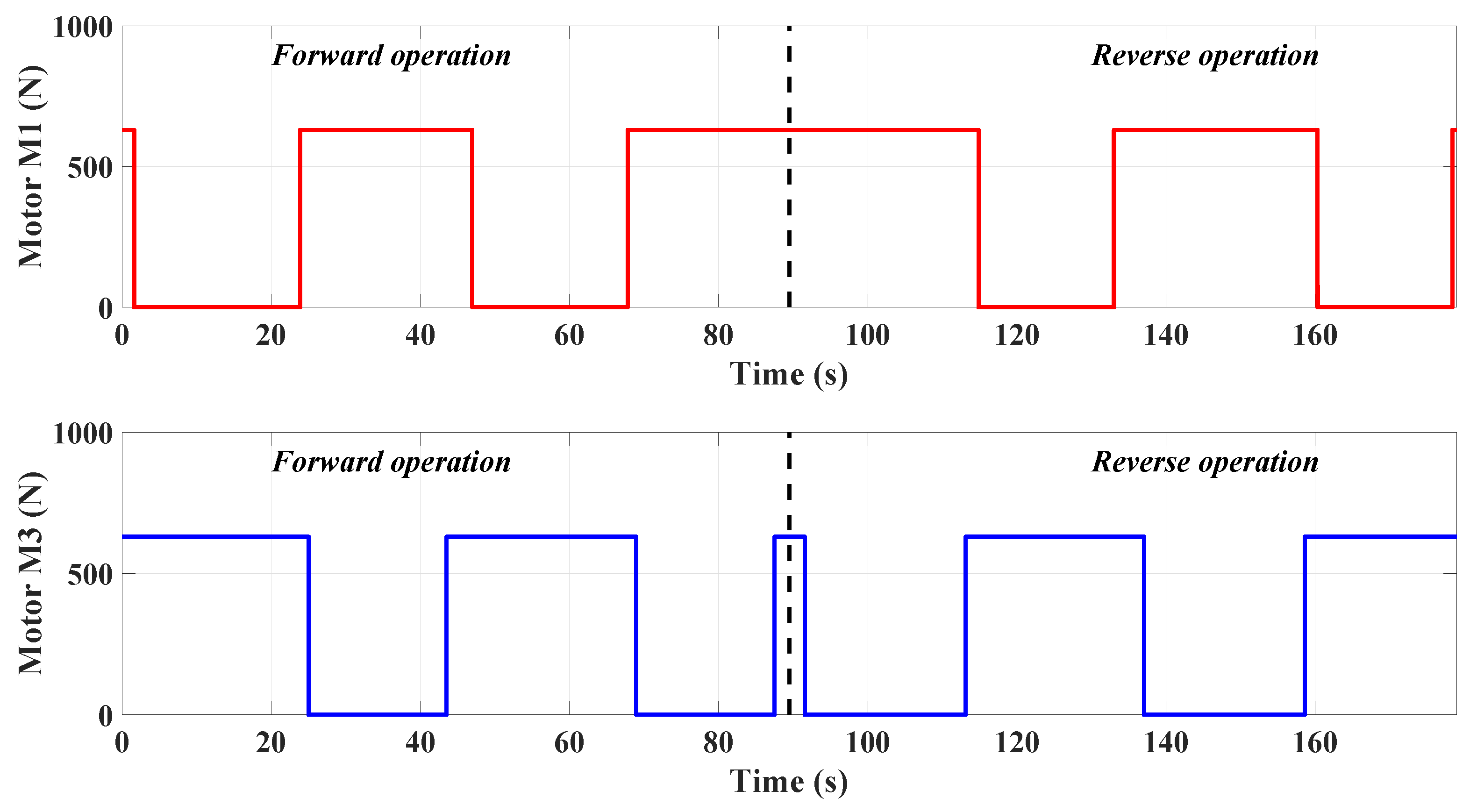
- Forward motion (twice)
- Reverse motion (twice)
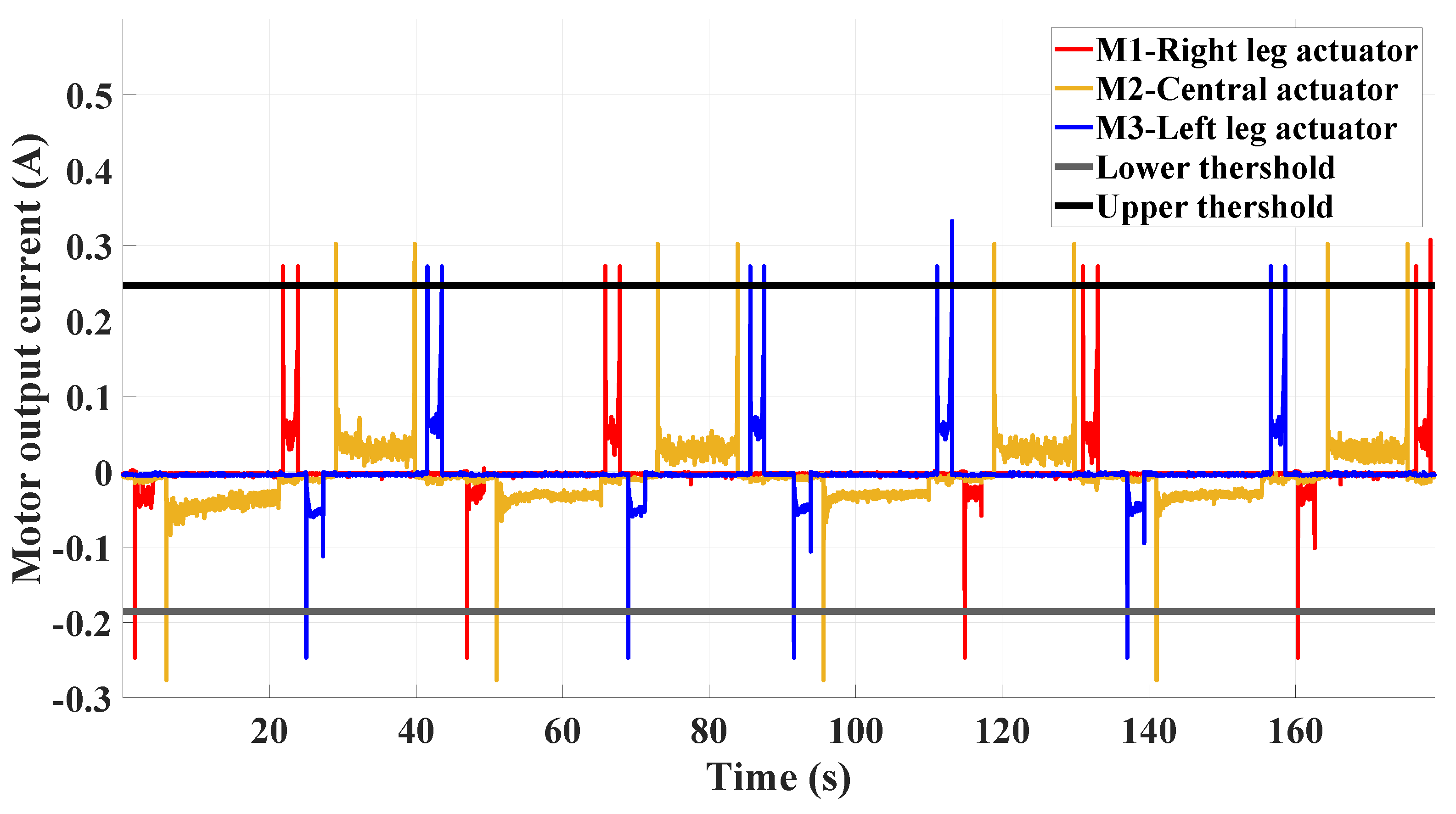
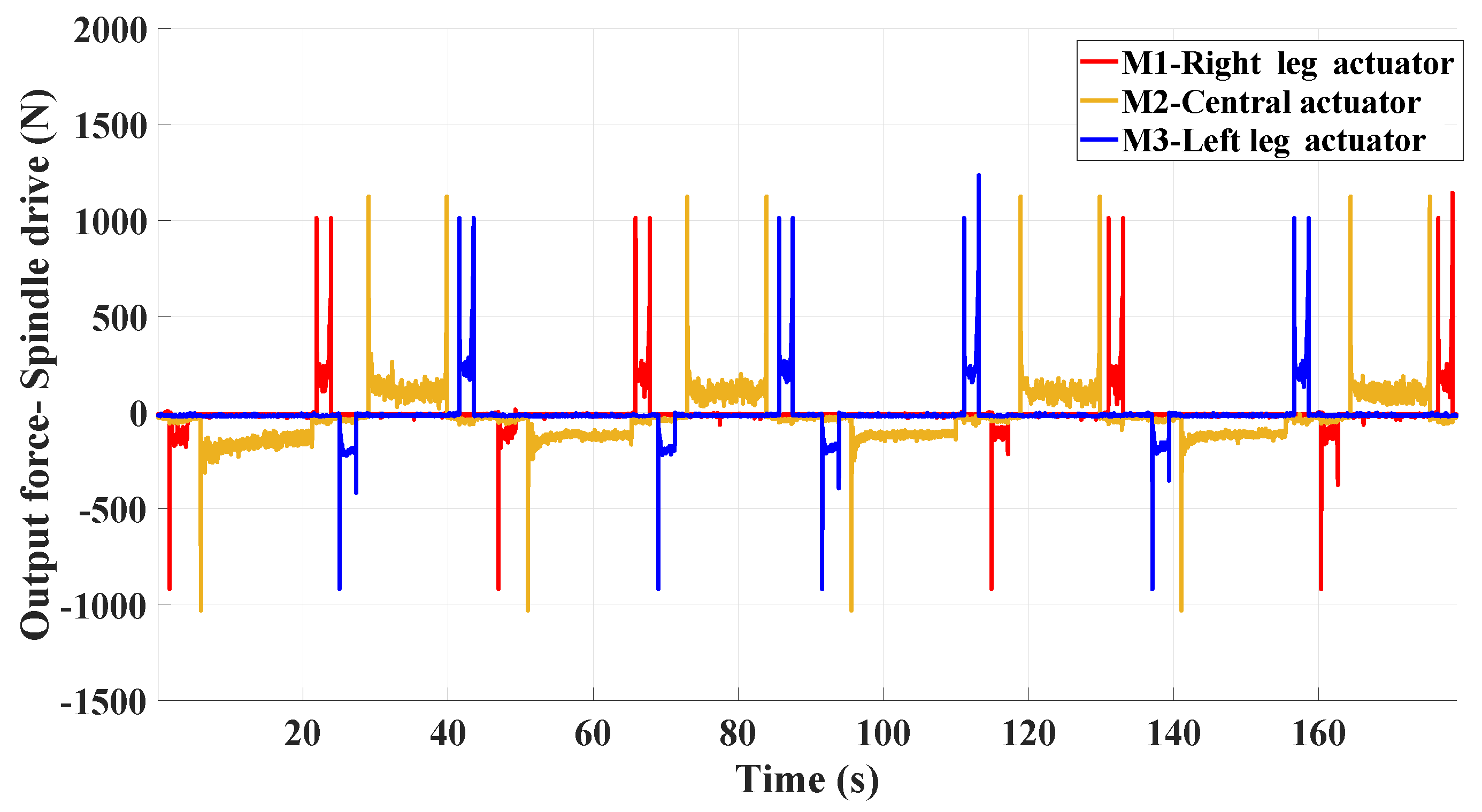
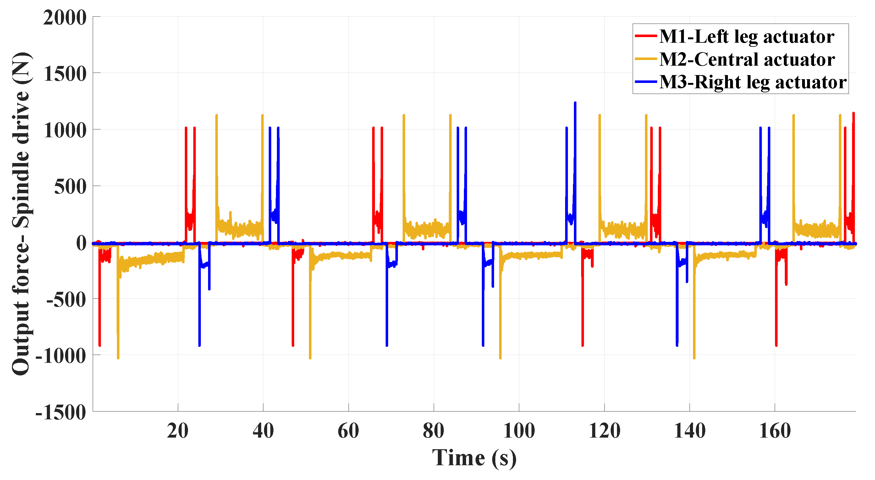
4.1. Estimation of Currents and Forces of the Motors from Experiments
5. Discussions
Author Contributions
Funding
Acknowledgments
Conflicts of Interest
Abbreviations
| DKM | Direct Kinematic Model |
| IKM | Inverse Kinematic Model |
| CG | Center of Gravity |
| PWM | Pulse width modulation |
| GPIO | General-purpose Input/Output |
| ADC | Analog to Digital convertor |
| BB | BeagleBone |
| Nomenclature | |
| Symbol | Description |
| Leg module actuation units | |
| Central module actuation unit | |
| Length of leg used in slot-follower mechanism | |
| Rotation angle of robot | |
| Rotation angle of pipeline | |
| Rotation matrix about z-axis | |
| Vector coordinates for | |
| l | CG distance between clamped points and free end |
| w | Self-weight of the robot |
| Force vector | |
| Moment vector | |
| Wrench at CG | |
| Tangential longitudinal force | |
| Tangential radial force | |
| Normal forces | |
| Coefficient of friction | |
| Magnitude of actuator force | |
| , | Magnitude of contact force/Total normal force |
| Force transmission factor | |
| I | Current induced on actuators |
| Magnitude of measured voltage at time t | |
| Magnitude of torque measured in experiments | |
| p | Pitch of screw in spindle drive |
| Output force of spindle drive |
Appendix

| Parameters | Value |
|---|---|
| Nominal voltage | 12 V |
| Nominal current () | 0.456 A |
| No load speed | 13,500 rpm |
| No load current () | 60.2 mA |
| Nominal speed | 5840 rpm |
| Efficiency () | 54% |
| Torque constant () | 7.82 mNm/A |
| Speed constant () | 1220 rpm/V |
| Terminal resistance | 15.7 |
| Parameters | Value |
|---|---|
| Spindle screw diameter and pitch (p) | 5 × 2 mm |
| Reduction ratio (G) | 455:1 |
| Max. static axial load | 500 N |
| Max. spindle length | 102 mm |
| Efficiency () | 63% |
References
- Kassim, I.; Phee, L.; Ng, W.S.; Gong, F.; Dario, P.; Mosse, C.A. Locomotion techniques for robotic colonoscopy. IEEE Eng. Med. Biol. Mag. 2006, 25, 49–56. [Google Scholar] [CrossRef] [PubMed]
- Takada, M. Self-Propelled Colonoscope. U.S. Patent 6,695,771, 24 February 2004. [Google Scholar]
- Masuda, S. Apparatus for Feeding a Flexible Tube through a Conduit. UK Patent 1,534,441, 6 December 1978. [Google Scholar]
- Hyun, J.; Hvung, J.; Young, M.; Juang, J.; Byungkyu, K.; Soo, H. Magnetic impact actuator for robotic endoscope. In Proceedings of the 32nd International Symposium on Robotics, Seoul, Korea, 19–21 April 2001; pp. 1834–1838. [Google Scholar]
- Iddan, G.J.; Sturlesi, D. In Vivo Video Camera System. U.S. Patent 5,604,531, 18 February 1997. [Google Scholar]
- Drapier, M.; Steenbrugghe, V.; Successeurs, B. Perfectionnements Aux Cathéters Médicaux. France Patent 1,278,965, 15 December 1961. [Google Scholar]
- Ikuta, K.; Tsukamoto, M.; Hirose, S. Shape memory alloy servo actuator system with electric resistance feedback and application for active endoscope. In Proceedings of the 1988 IEEE International Conference on Robotics and Automation, Philadelphia, PA, USA, 24–29 April 1988; pp. 427–430. [Google Scholar]
- Utsugi, M. Tubular Medical Instrument Having a Flexible Sheath Driven by a Plurality of Cuffs. U.S. Patent 4,148,307, 10 April 1979. [Google Scholar]
- Treat, M.R.; Trimmer, W.S. Self-Propelled Endoscope Using Pressure Driven Linear Actuators. U.S. Patent 5,595,565, 21 January 1997. [Google Scholar]
- Ginsburgh, I.; Carlson, J.A., III; Taylor, G.L.; Saghatchi, H. Method and Apparatus for Fluid Propelled Borescopes. U.S. Patent 4,735,501, 5 April 1988. [Google Scholar]
- Nayak, A.; Pradhan, S. Design of a new in-pipe inspection robot. Procedia Eng. 2014, 97, 2081–2091. [Google Scholar] [CrossRef]
- Zhang, Y.; Zhang, M.; Sun, H.; Jia, Q. Design and motion analysis of a flexible squirm pipe robot. In Proceedings of the 2010 International Conference on Intelligent System Design and Engineering Application, Changsha, China, 13–14 October 2010; pp. 527–531. [Google Scholar]
- Kwon, Y.S.; Lim, H.; Jung, E.J.; Yi, B.J. Design and motion planning of a two-moduled indoor pipeline inspection robot. In Proceedings of the 2008 IEEE International Conference on Robotics and Automation, Pasadena, CA, USA, 19–23 May 2008; pp. 3998–4004. [Google Scholar]
- Henry, R.; Chablat, D.; Porez, M.; Boyer, F.; Kanaan, D. Multi-objective design optimization of the leg mechanism for a piping inspection robot. In Proceedings of the ASME 2014 International Design Engineering Technical Conferences and Computers and Information in Engineering Conference, Buffalo, NY, USA, 17–20 August 2014. [Google Scholar]
- Chablat, D.; Venkateswaran, S.; Boyer, F. Mechanical Design Optimization of a Piping Inspection Robot. Procedia CIRP 2018, 70, 307–312. [Google Scholar] [CrossRef]
- Rao, R.V.; Waghmare, G. A new optimization algorithm for solving complex constrained design optimization problems. Eng. Optim. 2017, 49, 60–83. [Google Scholar] [CrossRef]
- Chablat, D.; Venkateswaran, S.; Boyer, F. Dynamic Model of a Bio-Inspired Robot for Piping Inspection. In ROMANSY 22–Robot Design, Dynamics and Control; Springer: Berlin/Heidelberg, Germany, 2019; pp. 42–51. [Google Scholar]
- Anthierens, C.; Ciftci, A.; Betemps, M. Design of an electro pneumatic micro robot for in-pipe inspection. In Proceedings of the IEEE International Symposium on Industrial Electronics (Cat. No.99TH8465), Bled, Slovenia, 12–16 July 1999; pp. 968–972. [Google Scholar]
- Anthierens, C.; Libersa, C.; Touaibia, M.; Bétemps, M.; Arsicault, M.; Chaillet, N. Micro robots dedicated to small diameter canalization exploration. In Proceedings of the 2000 IEEE/RSJ International Conference on Intelligent Robots and Systems (IROS 2000) (Cat. No.00CH37113), Takamatsu, Japan, 31 October–5 November 2000; pp. 480–485. [Google Scholar]
- Venkateswaran, S.; Chablat, D. CATIA Model of the Robot and Its Simulation. Available online: https://www.youtube.com/watch?v=7z6-by83mtw (accessed on 6 March 2019).
- Park, J.; Hyun, D.; Cho, W.H.; Kim, T.H.; Yang, H.S. Normal-force control for an in-pipe robot according to the inclination of pipelines. IEEE Trans. Ind. Electron. 2011, 58, 5304–5310. [Google Scholar] [CrossRef]
- Maxon Motors, Program 2017/18. High Precision Drives and Systems. Available online: http://epaper.maxonmotor.com/ (accessed on 15 December 2017).
- Ur-Rehman, R.; Caro, S.; Chablat, D.; Wenger, P. Multiobjective design optimization of 3-PRR planar parallel manipulators. In Proceedings of the 20th CIRP Design Conference, Nantes, France, 19–21 April 2010. [Google Scholar]
- Khalil, W.; Dombre, E. Modeling, Identification and Control of Robots; Hermes Penton Ltd.: London, UK, 2002. [Google Scholar]
- BeagleBone Black. Available online: https://elinux.org/Beagleboard:BeagleBoneBlack (accessed on 29 June 2018).
- Savitzky-Golay Filtering. Available online: https://fr.mathworks.com/help/signal/ref/sgolayfilt.html (accessed on 28 August 2018).
- Venkateswaran, S.; Chablat, D. Video of the Experiment on the Bio-Inspired Robot at 5x Speed. Available online: https://www.youtube.com/watch?v=EPpZa-hvFKI&t=4s (accessed on 10 April 2019).
- Venkateswaran, S.; Chablat, D. A new inspection robot for pipelines with bends and junctions. In Proceedings of the 15th IFToMM World Congress, Krakow, Poland, 30 June–4 July 2019. [Google Scholar]
- Venkateswaran, S.; Furet, M.; Chablat, D.; Wenger, P. Design and analysis of a tensegrity mechanism for a bio-inspired robot. In Proceedings of the ASME 2019 International Design Engineering Technical Conferences and Computers and Information in Engineering Conference, Anaheim, CA, USA, 18–21 August 2019. [Google Scholar]
- Arena, P.; Fortuna, L.; Frasca, M. Attitude control in walking hexapod robots: An analogic spatio-temporal approach. Int. J. Circuit Theory Appl. 2002, 30, 349–362. [Google Scholar] [CrossRef]


| Lengths | Dimensions [mm] |
|---|---|
| 57 | |
| 7 | |
| e | 11 |
| 8.5–45.5 |
| Position of Central Actuator | Radius of the Pipeline (mm) | Position of CG from Clamped End (mm) |
|---|---|---|
| Fully retracted | 27 | 128 |
| Fully extended | 27 | 149 |
| Fully retracted | 37 | 123 |
| Fully extended | 37 | 144 |
| Position of Central Actuator | Pipeline Radius (mm) | Actuator Force (N) Horizontal Pipe | Actuator Force (N) Vertical Pipe |
|---|---|---|---|
| Fully retracted | 27 | 60.6–63.7 | 20.4 |
| Fully extended | 27 | 68.8–73.1 | 20.4 |
| Fully retracted | 37 | 111.3–115 | 49.7 |
| Fully extended | 37 | 125.7–130.8 | 49.7 |
| PWM Duty Cycle | ADC Voltage Range (V) | Nominal cUrrent Settings (A) | Motor Speed (rpm) |
|---|---|---|---|
| 20% | 0 | −0.46 | 10,800 (Counter-clockwise) |
| 50% (idle) | 0.9 | 0 | 0 |
| 80% | 1.8 | 0.46 | 10,800 (Clockwise) |
| Orientation of Pipeline | Phase | Initial Force (N) | Final Force (N) | Force under Operation (N) |
|---|---|---|---|---|
| Horizontal | Clamping (M1 & M3) | 1000 | 1000 | 170–250 |
| Horizontal | Declamping (M1 & M3) | 900 | 0 | 80–150 |
| Vertical | Clamping (M1 & M3) | 1000 | 1000 | 160–330 |
| Vertical | Declamping (M1 & M3) | 900 | 0 | 100–180 |
| Horizontal & Vertical | Elongation (M2) | 1000 | 0 | 110–160 |
| Horizontal & Vertical | Retraction (M2) | 1100 | 1100 | 100–150 |
© 2019 by the authors. Licensee MDPI, Basel, Switzerland. This article is an open access article distributed under the terms and conditions of the Creative Commons Attribution (CC BY) license (http://creativecommons.org/licenses/by/4.0/).
Share and Cite
Venkateswaran, S.; Chablat, D.; Boyer, F. Numerical and Experimental Validation of the Prototype of a Bio-Inspired Piping Inspection Robot. Robotics 2019, 8, 32. https://doi.org/10.3390/robotics8020032
Venkateswaran S, Chablat D, Boyer F. Numerical and Experimental Validation of the Prototype of a Bio-Inspired Piping Inspection Robot. Robotics. 2019; 8(2):32. https://doi.org/10.3390/robotics8020032
Chicago/Turabian StyleVenkateswaran, Swaminath, Damien Chablat, and Frédéric Boyer. 2019. "Numerical and Experimental Validation of the Prototype of a Bio-Inspired Piping Inspection Robot" Robotics 8, no. 2: 32. https://doi.org/10.3390/robotics8020032
APA StyleVenkateswaran, S., Chablat, D., & Boyer, F. (2019). Numerical and Experimental Validation of the Prototype of a Bio-Inspired Piping Inspection Robot. Robotics, 8(2), 32. https://doi.org/10.3390/robotics8020032