Article

Model-Free Gradient-Based Adaptive Learning Controller for an Unmanned Flexible Wing Aircraft

1
School of Electrical Engineering and Computer Science, University of Ottawa, Ottawa, ON K1N 6N5, Canada
2
Department of Electrical Engineering, University of Texas at Arlington, Arlington, TX 76019, USA
*
Author to whom correspondence should be addressed.
Robotics 2018, 7(4), 66; https://doi.org/10.3390/robotics7040066
Submission received: 1 September 2018 / Revised: 19 October 2018 / Accepted: 20 October 2018 / Published: 23 October 2018
(This article belongs to the Special Issue Feature Papers)

Abstract

:
Classical gradient-based approximate dynamic programming approaches provide reliable and fast solution platforms for various optimal control problems. However, their dependence on accurate modeling approaches poses a major concern, where the efficiency of the proposed solutions are severely degraded in the case of uncertain dynamical environments. Herein, a novel online adaptive learning framework is introduced to solve action-dependent dual heuristic dynamic programming problems. The approach does not depend on the dynamical models of the considered systems. Instead, it employs optimization principles to produce model-free control strategies. A policy iteration process is employed to solve the underlying Hamilton–Jacobi–Bellman equation using means of adaptive critics, where a layer of separate actor-critic neural networks is employed along with gradient descent adaptation rules. A Riccati development is introduced and shown to be equivalent to solving the underlying Hamilton–Jacobi–Bellman equation. The proposed approach is applied on the challenging weight shift control problem of a flexible wing aircraft. The continuous nonlinear deformation in the aircraft’s flexible wing leads to various aerodynamic variations at different trim speeds, which makes its auto-pilot control a complicated task. Series of numerical simulations were carried out to demonstrate the effectiveness of the suggested strategy.

1. Introduction

Various Approximate Dynamic Programming (ADP) methods have been employed to solve the optimal control problems for single and multi-agent systems [1,2,3,4,5,6]. They are divided into different classes according to the way the temporal difference equations and the associated optimal strategies are evaluated. The ADP approaches that consider gradient-based forms provide fast converging approaches, but they require the complete knowledge of the dynamical model of the system under consideration [7]. The solution of the flexible wing control problem requires model-free approaches, since the aerodynamics of the flexible wing aircraft are highly nonlinear and they variate continuously [8,9,10,11,12,13,14,15,16]. This type of aircraft has large uncertainties embedded in their aerodynamic models. Herein, an online adaptive learning approach, based on a gradient structure, is employed to solve the challenging control problem of flexible wing aircrafts. This approach does not need any of the aerodynamic information of the aircraft. It is based on a model-free control strategy approximation.
Several ADP approaches have been adopted to solve the difficulties associated with the dynamic programming solutions which involve the curse of dimensionality in the state and action spaces [2,3,4,5,17,18]. They are employed in different applications such as machine learning, autonomous systems, multi-agent systems, consensus and synchronization, and decision making problems [19,20,21]. Typical optimal control methods tend to solve the underlying Hamilton–Jacobi–Bellman (HJB) equation of the dynamical system by applying the optimality principles [22,23]. An optimal control problem is usually formulated as an optimization problem with a cost function that identifies the optimization objectives and a mathematical process to find the respective optimal strategies [6,7,18,22,23,24,25,26,27,28]. To implement the optimal control solutions stemming from the ADP approaches, numerous solving frameworks are considered based on combinations of Reinforcement Learning (RL) and adaptive critics [1,5,18,25,27]. Reinforcement Learning approaches use various forms of temporal difference equations to solve the optimization problems associated with the dynamical systems [1,18]. This implies finding ways to penalize or reward the attempted control strategies to optimize a certain objective function. This is accomplished in a dynamic learning environment where the agent applies its acquired knowledge to update its experience about the merit of using the attempted policies. RL methods implement the temporal difference solutions using two main coupled steps. The first approximates the value of a given strategy, while the second approximates the optimal strategy itself. The sequence of these coupled steps can be implemented with either value or policy iteration method [18]. RL has also been proposed to solve problems with multi-agent structures and objectives [29] as well as cooperative control problems using dynamic graphical games [21,26,30]. Action Dependent Dual Heuristic Dynamic Programming (ADDHP) depends on the system’s dynamic model [7,26,28]. Herein, the relation between the Hamiltonian and Bellman equation is used to solve for the governing costate expressions and hence a policy iteration process is proposed to find an optimal solution. Dual Heuristic Dynamic Programming (DHP) approaches for graphical games are developed in [21,26,30]. However, these approaches require in-advance knowledge of the system’s dynamics and, in some cases of the multi-agent systems, they rely on complicated costate structures to include the neighbors influences.
Adaptive critics are typically implemented within reinforcement learning solutions using neural network approximations [18,27]. The actor approximates the optimal strategy, while the value of the assessed strategy is approximated by the critic [18]. Real-time optimal control solutions using adaptive critics are introduced in [3]. Adaptive critics provide prominent solution frameworks for the adaptive dynamic programming problems [31]. They are employed to produce expert paradigms that can undergo learning processes while solving the underlying optimization challenges. Moreover, they have been invoked to solve a wide spectrum of optimal control problems in continuous and discrete-time domains, where actor-critic schemes are evoked within an Integral Reinforcement Learning context [32,33]. An action-dependent solving value function is proposed to play some zero-sum games in [34], where one critic and two actors are adapted forward in time to solve the game. An online distributed actor-critic scheme is suggested to implement a Dual Heuristic Dynamic Programming solution for the dynamic graphical games in [7,24] without overlooking the neighbors’ effects, which is a major concern in the classical DHP approaches. The solution provided by each agent is implemented by single actor-critic approximators. Another actor-critic development is applied to implement a partially-model-free adaptive control solution for a deterministic nonlinear system in [35]. A reduced solving value function approach employed an actor-critic scheme to solve the graphical games, where only partial knowledge about the system dynamics is necessary [26]. An actor-critic solution framework is adopted for an online policy iteration process with a weighted-derivative performance index form in [33]. A model-free optimal solution for graphical games is implemented using only one critic structure for each agent in [25]. The recent state-of-the-art adaptive critics implementations for numerous reinforcement learning solutions for the feedback control problems are surveyed in [36]. These involve the regulation and tracking problems for single- as well as multi-agent systems [36].
Flexible wing aircraft are usually modeled as two-mass systems (fuselage and wing). Both masses are coupled via different kinematic and dynamic constraints [8,13,14,15,37]. They involve the kinematic constraint at the connection point of the hang strap [38,39]. The keel tube works as a symmetric axis for this type of aircraft. The basic theoretical and experimental developments for the aerodynamic modeling aspects of the flexible wing systems are introduced in [8,13,14,15,40,41]. Several wind tunnel experiments have been introduced for the hang glider in [14]. An approximate modeling approach of the flexible wing’s aerodynamics led to equations of motion for the lateral and longitudinal directions with small perturbation models in [42]. The modeling process for the hang glider assumed a rigid wing modeling process, where the derivatives, due to the aerodynamics, were added at the last stage [11,12]. A comprehensive decoupled aerodynamic model for the hang glider is presented in [43]. A nine-degree-of-freedom aerodynamic model that employs a set of nonlinear state equations is developed in [38,39]. The control of the flexible wing aircraft follows a weight shift mechanism, where the lateral and longitudinal maneuvers or the roll/pitch control mechanism is achieved by changing the relative centers of gravity of the wing and the fuselage systems [9,10,13,14,37,44]. The geometry of the flexible wing’s control arm influences the maximum allowed control moments [9]. The reduced center of gravity magnifies the static pitch stability [9]. Frequency response-based approaches are adopted to study the stability of flexible wing systems in [11,12]. The longitudinal stability of a fixed wing system can be used to understand that of the flexible wing vehicle provided some conditions are satisfied [37]. The lateral stability margins are shown to be larger compared to conventional fixed wing aircraft.
The contribution of this work is four-fold:
  • An online adaptive learning control approach is proposed to solve the challenging weight-shift control problem of flexible wing aircraft. The approach uses model-free control structures and gradient-based solving value functions. This serves as a model-free solution framework for the classical Action Dependent Dual Heuristic Dynamic Programming problems.
  • The work handles many concerns associated with implementing value and policy iteration solutions for ADDHP problems, which either necessitate partial knowledge about the system dynamics or involve difficulties in the evaluations of the associated solving value functions.
  • The relation between a modified form of Bellman equation and the Hamiltonian expression is developed to transfer the gradient-based solution framework from the Bellman optimality domain to an alternative domain that uses Hamilton–Jacobi–Bellman expressions. This duality allows for a straightforward solution setup for the considered ADDHP problem. This is supported by a Riccati development that is equivalent to solving the underlying Bellman optimality equation.
  • The proposed solution that is based on the combined-costate structure is implemented using a novel policy iteration approach. This is followed by an actor-critic implementation that is free of the computational expensive matrix inverse calculations.
The paper is organized as follows: Section 2 briefly explains the weight shift control mechanism of a flexible wing aircraft. Section 3 highlights the model-based solutions within the framework of optimal control theory along with the existing challenges. Section 4 discusses the duality between the Hamiltonian function and Bellman equation leading to the Hamilton–Jacobi–Bellman formulation, which is used to generalize the Action Dependent Dual Heuristic Dynamic Programming solution with a policy iteration process. Section 5 introduces the model-free gradient-based solution and the underlying Riccati development. Section 6 demonstrates the adaptive critics implementations for the proposed model-free gradient-based solution. Section 7 tests the validity of the introduced online adaptive learning control approach by applying it on two case studies. Finally, the paper is concluded with some concluding remarks in Section 8.

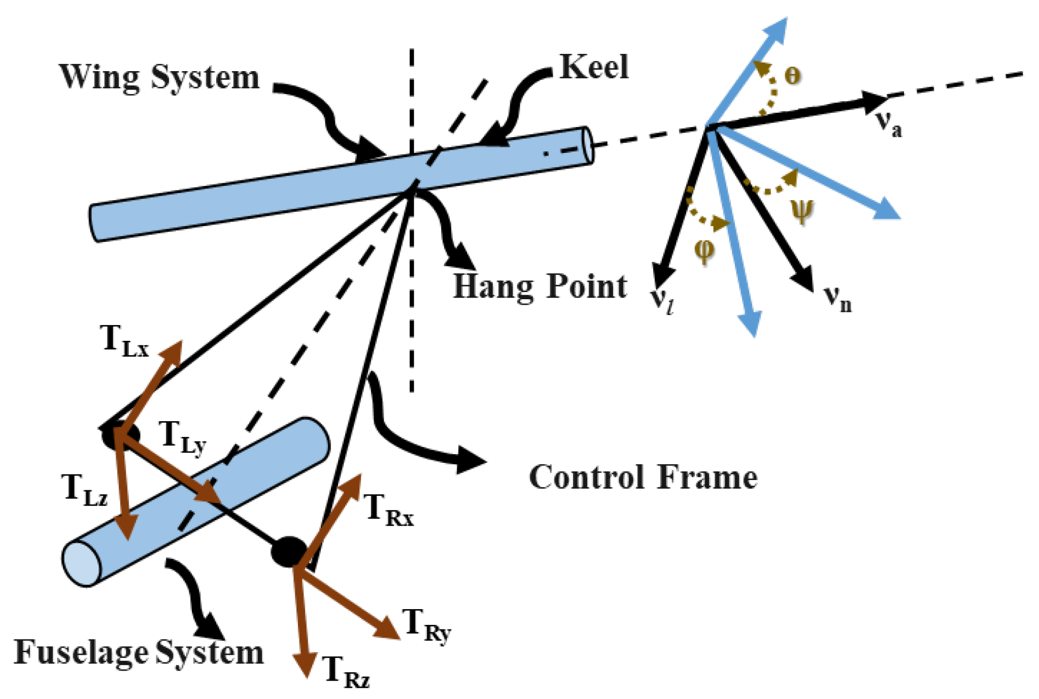
2. Control Mechanism of a Flexible Wing Aircraft

This section briefly introduces the idea of weight shift control along with a basic aerodynamic model of a flexible wing system. Herein, a flexible wing aircraft is modeled as a two-mass system (fuselage/pilot and wing) coupled through nonlinear kinematic constraints at the hang strap, as shown in Figure 1. The flexible wing is connected to the fuselage through a control bar. The aerodynamic forces are controlled via a weight shift mechanism, where the fuselage’s center of gravity “floats” with respect to that of the wing [8,9,10,11,12,37,44]. Such a system is governed by complex aerodynamic forces which makes it difficult to model to a satisfactory accuracy. Consequently, model-based control approaches may not be appropriate for the auto-pilot control of such systems.
In this framework, the longitudinal and lateral motions are controlled through the force components applied on the control bar of the hang glider [38,39]. This development takes into account a nine-degree-of-freedom model that considers the kinematic interactions and the constraints between the fuselage and the wing at the hang point, as shown in Figure 1. The longitudinal and lateral dynamics are referred to the wing’s frame, where the forces (nonlinear state equations) at the hang point are substituted for by some transformations in the wing’s frame [39].
The decoupled longitudinal and lateral aerodynamic models satisfy the following assumptions [39]:
  • The hang strap works as a kinematic constraint between the decoupled wing/fuselage systems.
  • The fuselage system is assumed to be a rigid body connected to the wing system via a control triangle and a hang strap.
  • The force components applied on the control bar are the input control signals.
  • External forces, such as the aerodynamics and gravity, the associated moments, and the internal forces, are evaluated for both fuselage and wing systems.
  • The fuselage’s pitch–roll–yaw attitudes and pitch–roll–yaw attitude rates are referred to the wing’s frame of motion through kinematic transformations.
  • The complete aerodynamic model of the aircraft is reduced by substituting for the internal forces at the hang strap using the action/reaction laws.
  • The pilot’s frames of motion (i.e., longitudinal and lateral states) are referred to the respective wing’s frames of motion.
The dynamics of the flexible wing aircraft are decoupled into longitudinal and lateral systems, such that [9,37,39,44].
δ ( k + 1 ) L o / L a = A L o / L a δ k L o / L a + B L o / L a u k L o / L a ,
where δ L o = [ ν a w ν n w θ ˙ w θ ˙ f w θ f w θ w ] T is the longitudinal state vector, δ L a = [ ν l w ϕ ˙ w ψ ˙ w ϕ ˙ f w ψ ˙ f w ϕ f w ψ f w ϕ w ] T is the lateral state vector, the force T c q = 1 2 T R q + T L q is the collective force in direction q, the force T d q = 1 2 T R q T L q is the differential force in direction q, u L o = [ T c x T c z ] T represents the longitudinal control signals, and u L a = [ T c y T d x T d z ] T denotes the lateral control signals.
The modeling results of the flexible wing aircraft are based on the experimental and theoretical studies of [9], where the control mechanism employs force components on the control bar [39].

3. Optimal Control Problem

This section explains the main challenges associated with the optimal solution of the control problem using Action Dependent Dual Heuristic Dynamic Programming approaches. It should justify the need for a model-free gradient-based optimal control solution.

3.1. Bellman Equation Formulation

Consider a flexible wing hang glider characterized by the following discrete-time state space equation:
δ k + 1 = A δ k + B u k ,
where δ k R n is a vector of the (longitudinal/lateral) states and u k R m is a vector of the (longitudinal/lateral) force components applied on the control bar, A and B are the (longitudinal/lateral) state space matrices, and k is the time index.
A quadratic convex performance index is introduced to assess the quality of the taken control actions, such that
J = k = 0 F ( δ k , u k ) ,
where F is a convex utility function given by
F ( δ k , u k ) = 1 2 δ k T Q δ k + u k T R u k ,
where Q 0 R n × n and R > 0 R m × m are symmetric time-invariant positive semi-definite and positive definite weighting matrices, respectively.
The structure in Equation (3) is used to suggest a solution form. First, the solving value function V ( δ k , u k ) is assumed to depend on the the state δ k and the control strategy u k so that
V ( δ k , u k ) = i = k F ( δ i , u i ) .
This yields a temporal difference (Bellman) equation defined by
V ( δ k , u k ) = 1 2 δ k T Q δ k + u k T R u k + V ( δ k + 1 , u k + 1 ) .
The value function in Equation (5) is assumed to have the following form
V ( δ k , u k ) = 1 2 [ δ k T u k T ] S δ k u k ,
where S = S δ δ S δ u S u δ S u u .

3.2. Model-Based Policy Formulation

Herein, a model-based optimal control strategy and the associated costate equation are derived by applying the Bellman’s optimality principles to Bellman equation (Equation (6)). Below, a model-free policy solution is introduced. To evaluate the optimal control strategy, the optimality principles are applied to V ( ) .
argmin u k V ( δ k , u k ) = V ( δ k , u k ) u k = 0 u o = R 1 B T I n × n u k + 1 δ k + 1 T δ u k + 1 V ( δ k + 1 , u k + 1 ) ,
where δ u k + 1 V ( δ k + 1 , u k + 1 ) = S · [ δ k + 1 T u k + 1 T ] T . Applying this model-based optimal policy in Equation (6) yields the following Bellman’s optimality equation:
V o δ k , u k o = 1 2 δ k T Q δ k + u k o T R u k o + V o δ ( k + 1 ) , u ( k + 1 ) o .
The gradient-based solution requires the knowledge of the costate equation associated with the system in Equation (2). The costate equation is evaluated as follows
δ k V ( δ k , u k ) = Q δ k + A T I n × n u k + 1 δ k + 1 T δ u k + 1 V ( δ k + 1 , u k + 1 ) ,
The main concern about this gradient-based development is that both the optimal strategy in Equation (8) and the associated costate Equation (10) depend on the dynamical model of the system (i.e., A and B). The following development shows how it is possible to avoid this shortcoming using dynamical information in deciding on the optimal control strategies.

3.3. Model-Free Policy Formulation

In the sequel, a model-free policy structure is introduced along with the optimal control solution algorithms. Applying the Bellman’s optimality principles [22] yields the optimal control strategy u k o so that
argmin u k V ( δ k , u k ) = argmin u k 1 2 [ δ k T u k T ] S δ k u k .
Note that the optimality principle is applied to the left-hand-side of Equation (6). This yields the following model-free control policy
u k o = K · δ k ,
where the control gain K is given by K = S u k u k 1 · S u k δ k . Substituting Equation (11) into Equation (6) yields a dual (equivalent) Bellman’s optimality equation (Equation (9)). The Bellman optimality equation (Equation (9)) will be used to propose different Action Dependent Dual Heuristic Dynamic solutions for the optimal control problem in hand, as shown below.
To propose gradient-based solutions, the gradient of the Bellman equation (Equation (6)) with respect to the state δ k is calculated.
δ k V ( δ k , u k ) = Q δ k + A T I n × n K T δ u k + 1 V ( δ k + 1 , u k + 1 ) ,
where δ k V ( δ k , u k ) = V ( δ k , u k ) / δ k and δ u k V ( δ k , u k ) = S · [ δ k T u k T ] T , k .
The optimal strategy (Equation (11)) and the costate (Equation (12)) are used to propose different gradient-based solution forms. These are generalizations of the ADDHP solution, where a slight modification on the approximation of the control policy is introduced. In the sequel, solutions based on value iteration and policy iteration processes are presented.
Remark 1.
Although Algorithm 1 and 2 use model-free policy structures (Equations (14) and (16)), the gradient expressions (Equations (13) and (15)) depend on the system’s drift dynamics (matrix A), which is a real challenge for systems with uncertain or unknown dynamics. Moreover, it is difficult to evaluate the matrix S, and so V, in Equation (15) using the policy iteration process. As such, a new approach is required to benefit the gradient-based solution form without the need for a system’s dynamic model. To do that, a dual development using the Hamiltonian framework is needed.
Algorithm 1 Value Iteration Gradient-based Solution
  • Initialize δ k V 0 ( δ k , u k ) and u k o .
  • Evaluate δ k V + 1 ( . . ) using
    δ k V + 1 ( δ k , u k ) = Q δ k + A T I n × n K T δ u k V ( δ k + 1 , u k + 1 ) ,
    where is the iteration index.
  • Update the approximation of the optimal strategy using
    u k + 1 = S u k u k 1 · S u k δ k + 1 · δ k .
  • Halt on convergence of S + 1 ( . . ) S ( . . ) .
Algorithm 2 Policy Iteration Gradient-based Solution
  • Initialize δ k V 0 ( δ k , u k ) and use admissible u k o .
  • Evaluate δ k V ( . . ) using
    δ k V ( δ k , u k ) = Q δ k + A T I n × n K T δ u k V ( δ k + 1 , u k + 1 ) .
  • Update the approximation of the optimal strategy using
    u k + 1 = S u k u k 1 · S u k δ k · δ k .
  • Halt on convergence of S + 1 ( . . ) S ( . . ) .

4. Hamiltonian-Jacobi–Bellman Formulation

The following Hamilton–Jacobi and Hamilton–Jacobi–Bellman developments are necessary to propose the model-free ADDHP control solutions. They find the relation between the costate variable of the Hamiltonian function and the solving value function through Bellman equation via a Hamilton–Jacobi framework. Then, the Hamilton–Jacob-Bellman development is used to propose the model-free ADDHP solution.

4.1. The Hamiltonian Mechanics

Optimal control problems, in general, are solved using the Hamiltonian mechanics, where the necessary conditions of optimality are found by means of Lagrange dynamics [22]. The objective of the optimization problem is to chose a policy μ k to minimize a cost function F such that argmin μ k F ( δ k , μ k ) , subject to the following constraints:
μ k = χ ( δ k ) = C δ k , δ ( k + 1 ) ϱ ( δ k , μ k ) ,
where χ R m × 1 and ϱ R n × 1 are some mapping functions, and C R m × n is a row gain matrix.
The Hamiltonian expression for the problem is given by
H ( δ k , λ ( k + 1 ) , μ k ) = λ ( k + 1 ) T δ k + 1 μ k + 1 + F ( δ k , μ k ) ,
where λ k R ( n + m ) × 1 is the Lagrange multiplier or the costate variable. Merging Equation (17) into Equation (18) leads to
H ( δ k , λ ( k + 1 ) , μ k ) = λ ( k + 1 ) T I n × n C δ k + 1 + F ( δ k , μ k ) .
Remark 2.
Similar to the optimal policy in Equation (8) derived using Bellman equation (Equation (6)), an optimal model-based control strategy based on the Hamiltonian can be obtained so that
argmin μ k H ( δ k , δ μ k + 1 V ( δ k + 1 , μ k + 1 ) , μ k ) = H ( ) μ k = 0 μ * = R 1 B T I n × n μ k + 1 δ k + 1 T δ μ k + 1 V ( δ k + 1 , μ k + 1 ) .
The following Hamilton–Jacobi theorem finds the relation between the costate variable λ k and the value function V ( δ k , u k ) , k .
Theorem 1.
Let the Hamiltonian function be given by Equation (18) and the value function V δ k , μ k be defined by Equation (6). Then, this value function satisfies the following Hamilton–Jacobi equation:
V δ k + 1 , μ k + 1 V δ k , μ k + H δ k , δ μ k + 1 V ( δ k + 1 , μ k + 1 ) , μ k δ μ k + 1 V ( δ k + 1 , μ k + 1 ) T δ k + 1 μ k + 1 = 0 ,
where λ k + 1 = δ μ k + 1 V ( δ k + 1 , μ k + 1 ) .
Proof. 
The augmented value function V ( δ k , μ k ) is
V δ k , μ k = l = k F δ k , μ k + λ ( l + 1 ) T I n × n C ϱ ( δ , μ ) δ ( l + 1 ) .
The Hamiltonian in Equation (18) is rearranged such that
H ( δ , λ ( + 1 ) , μ ) = λ ( + 1 ) T I n × n C δ + 1 + F ( δ , μ ) .
Using this expression into the augmented function in Equation (22) yields
V δ k + 1 , μ k + 1 V δ k , μ k + H δ k , λ ( k + 1 ) , μ k λ ( k + 1 ) T I n × n C δ ( k + 1 ) = 0 .
Finding the gradient of Equation (23) with respect to δ ( k + 1 ) yields
δ k + 1 V δ k + 1 , μ k + 1 + λ k + 1 δ k + 1 T H δ k , λ k + 1 , μ k λ k + 1 λ k + 1 δ k + 1 T I n × n C δ k + 1 + I n × n C T λ k + 1 = 0 .
This equation can be rearranged such that
δ k + 1 V δ k + 1 , μ k + 1 I n × n C T λ k + 1 + λ k + 1 δ k + 1 T H δ k , λ k + 1 , μ k λ k + 1 I n × n C δ k + 1 = 0 .
H δ k , λ k + 1 , μ k λ k + 1 = I n × n C δ k + 1 δ k + 1 V δ k + 1 , μ k + 1 = I n × n C T λ k + 1 .
This expression is equivalent to
[ I n × n C T ] S δ k + 1 μ k + 1 = I n × n C T λ k + 1 ,
which yields
λ k + 1 = S δ k + 1 μ k + 1 .
Then, the costate variable λ k + 1 can be written in terms of the gradient of the value function δ u k + 1 V ( ) , such that
λ k + 1 = δ μ k + 1 V ( δ k + 1 , μ k + 1 ) = V ( δ k + 1 , μ k + 1 ) δ k + 1 V ( δ k + 1 , μ k + 1 ) μ k + 1 .
Therefore, the value function V ( ) satisfies the HJ equation (Equation (21)). □

4.2. Hamiltonian–Bellman Solutions Duality

The following results show the conditions at which the Hamiltonian and Bellman-based solutions are dual.
Theorem 2.
(a) Let V ^ satisfy the following Hamilton–Jacobi–Bellman equation
H δ k , δ u k + 1 V ^ ( δ k + 1 , u k + 1 o ) , u k o = 0
δ u k + 1 V ^ ( δ k + 1 , u k + 1 o ) T δ k + 1 u k + 1 o + F ( δ k , u k o ) = 0 ,
with V ^ ( 0 ) = 0 , where
u o = R 1 B T I n × n u k + 1 δ k + 1 T δ u k + 1 V ^ ( δ k + 1 , u k + 1 ) .
Then, V ^ ( ) satisfies the Bellman optimality (Equation (9)).
(b) Let ( A , B ) be reachable. If V * ( ) satisfies Equation (9), then it satisfies the Hamilton–Jacobi–Bellman Equation (25).
Proof. 
(a) The value function V ^ δ k with the optimal policy u o  (Equation (27)) satisfies the HJB equation (Equation (25)). Then, Theorem 1 yields
V ^ δ k + 1 , u k + 1 o V ^ δ k , u k o = δ u k + 1 o V ^ ( δ k + 1 , u k + 1 o ) T δ k + 1 u k + 1 o .
Therefore, V ^ ( ) satisfies Equation (9).
(b) The Hamiltonian with the value function V ^ ( ) , arbitrary policy u k , and optimal policy u k o , evaluated using the optimal value function V ^ ( ) yields
H δ k , δ u k + 1 V ^ ( δ k + 1 , u k + 1 ) , u k = H δ k , δ u k + 1 V ^ ( δ k + 1 , u k + 1 o ) , u k o + 1 2 ( u k u k o ) T R ( u k u k o ) + δ u k + 1 V ^ ( δ k + 1 , u k + 1 ) T δ k + 1 u k + 1 δ u k + 1 V ^ ( δ k + 1 , u k + 1 o ) T δ k + 1 u k + 1 o .
H δ k , δ u k + 1 V ^ ( δ k + 1 , u k o ) , u k + 1 o = 0 . Then,
H δ k , δ u k + 1 V ^ ( δ k + 1 , u k + 1 ) , u k = 1 2 ( u k u k o ) T R ( u k u k o ) + δ u k + 1 V ^ ( δ k + 1 , u k + 1 ) T δ k + 1 u k + 1 δ u k + 1 V ^ ( δ k + 1 , u k + 1 o ) T δ k + 1 u k + 1 o .
Bellman equation (Equation (6)) can be rearranged such that
V ( δ k , u k ) = 1 2 δ k T Q δ k + u k T R u k + V ( δ k + 1 , u k + 1 ) + δ u k + 1 V ^ ( δ k + 1 , u k + 1 ) T δ k + 1 u k + 1 δ u k + 1 V ^ ( δ k + 1 , u k + 1 ) T δ k + 1 u k + 1 .
Equations (28) and (29), and the results from Theorem 1, yield
V ( δ k , u k ) = V ( δ k + 1 , u k + 1 ) + 1 2 ( u k u k o ) T R ( u k u k o ) δ u k + 1 V ^ ( δ k + 1 , u k + 1 o ) T δ k + 1 u k + 1 o .
Applying the optimality principles (i.e., taking the derivative of V ( ) with respect to u k ) leads to the optimal value function V * ( ) and the respective optimal policy u k * .
V ( δ k , u k ) u k = 0 u k * u k o = R 1 B T × I n × n u k + 1 δ k + 1 T δ u k + 1 V * ( δ k + 1 , u k + 1 ) u = u * I n × n u k + 1 δ k + 1 T δ u k + 1 V ^ ( δ k + 1 , u k + 1 ) u = u o .
The Hessian of the Hamiltonian (as a function of δ k , V ^ ( ) and u k ) and the Hessian of the Bellman equation (as a function of δ k , V * ( ) and u k ) are given by
2 H ( ) u k 2 = 2 V ^ ( ) u k 2 = R + B T I n × n u k + 1 δ k + 1 T S ^ I n × n u k + 1 δ k + 1 B , 2 V * ( ) u k 2 = R + B T I n × n u k + 1 δ k + 1 T S * I n × n u k + 1 δ k + 1 B ,
where S ^ > 0 and S * > 0 are the positive-definite solution matrices associated with V ^ ( ) and V * ( ) , respectively.
Thus, 2 H ( ) / u k 2 > 0 and 2 V ^ ( ) / u k 2 > 0 . Therefore, the optimal policies u k * and u k o are unique and u k * = u k o . Consequently, according to Equation (30), V * ( ) satisfies the HJB equation (Equation (25)) (i.e., V * ( ) = V ^ ( ) ) if the system is reachable. This can be explained by incorporating the difference between the costate equations evaluated by the Hamiltonian function and Bellman Equation in Equation (30) so that
δ k V * ( δ k , u k ) δ k V ^ ( δ k , u k ) = A T I n × n u k + 1 δ k + 1 T δ u k + 1 V * ( δ k + 1 , u k + 1 ) u = u * I n × n u k + 1 δ k + 1 T δ u k + 1 V ^ ( δ k + 1 , u k + 1 ) u = u o .
These results conclude the duality between the Hamiltonian function and Bellman equation for the Action Dependent Dual Heuristic Dynamic Programming solutions. □

5. The Adaptive Learning Solution and Riccati Development

This section introduces the online gradient-based model-free adaptive learning solution which uses the previous HJB development. Then, a Riccati development for the underlying optimal control problem is introduced (it is equivalent to solving the underlying Bellman’s optimality (Equation (9)) or the HJB equation (Equation (25)).

5.1. Model-Free Gradient-Based Solution

The results of Theorem 2 are used to develop a gradient-based algorithm which generalizes the ADDHP solution for the optimal control problem using a model-free policy structure. This adaptive learning solution is based on an online policy iteration process. The duality between the Hamilton–Jacobi–Bellman (HJB) equation (Equation (25)) and Bellman optimality (Equation (9)) is leveraged to propose a gradient-based approach that leads to a model-free control strategy. Algorithm 3 is as follows:
Algorithm 3 Online Policy Iteration Process
  • Initialize the costate V 0 ( δ k ) and the policy u k o .
  • Evaluate δ u V ( . . )
    δ u k + 1 V ( δ k + 1 , u k + 1 ) T δ k + 1 u k + 1 = F ( δ k , u k ) .
  • Update the approximation of the optimal strategy,
    u k + 1 = S u k u k 1 · S u k δ k · δ k .
  • Terminate on convergence of V + 1 ( . . ) V ( . . ) .

5.2. Riccati Development

The following result shows the equivalent Riccati development of the underlying optimal control solution.
Theorem 3.
Let the solution of Equation (9), or equivalently Equation (25), be given by V ( δ k , u k ) = 1 2 [ δ k T u k T ] Ψ δ k u k and the optimal strategy follows Equation (8). Then, there is a Riccati solution that is given by
Ψ r + 1 = Q + A cT Ψ ˜ r A c A T Ψ ˜ r B c B cT Ψ ˜ r A c R + B cT Ψ ˜ r B c .
Note that the parameters of Equation (33) are defined in the proof below.
Proof. 
The optimal policy in Equation (8) can be written as u k = Ψ ^ δ k , where Ψ = Ψ δ δ Ψ δ u Ψ u δ Ψ u u and Ψ ^ = Ψ u u 1 Ψ u δ .
Therefore, the value function V ( k + 1 ) can be expressed as
V δ ( k + 1 ) , u ( k + 1 ) = 1 2 δ ( k + 1 ) T Ψ ˜ δ ( k + 1 ) ,
where Ψ ˜ = Ψ δ δ Ψ δ u Ψ u u 1 Ψ u δ .
Substituting the policy in Equation (8) and the value function (Equation (34)) into Equation  (2), yields
δ ( k + 1 ) = A δ k B R 1 B T Ψ ˜ ( A δ k + B u k ) .
Then,
δ ( k + 1 ) = A c δ k + B c u k ,
where A c = A B R 1 B T Ψ ˜ A and B c = B R 1 B T Ψ ˜ B .
Substituting Equations (35) and (34) into Bellman equation (Equation (9)) leads to
V δ k , u k = 1 2 δ k T Q δ k + u k T R u k + 1 2 δ k T A cT Ψ ˜ A c δ k + 1 2 u k T B cT Ψ ˜ B c u k + 1 2 u k T B cT Ψ ˜ A c δ k + 1 2 δ k T A cT Ψ ˜ B c u k .
Therefore,
[ δ k T u k T ] Ψ δ k u k = [ δ k T u k T ] Q + A cT Ψ ˜ A c A T Ψ ˜ B c B cT Ψ ˜ A c R + B cT Ψ ˜ B c δ k u k .
Then,
Ψ = Q + A cT Ψ ˜ A c A T Ψ ˜ B c B cT Ψ ˜ A c R + B cT Ψ ˜ B c .
This equation yields the Riccati form of Equation (33). □

6. Adaptive Critics Implementations

This section shows the neural network approximation for the online policy iteration solution proposed by Algorithm 3. This implementation represents the optimal value approximation separately form the policy approximation. However, they are both coupled through the Bellman equation or the Hamiltonian function.

6.1. Actor-Critic Neural Networks Implementation

Herein, a simple layer of actor and critic neural network structures is considered. The actor is used to approximate the optimal strategy of Equation (32) while the critic approximates the optimal value in Equation (31). The learning environment involves selecting the values that minimize a cost function along with the associated approximation of the optimal strategies resulting from the feedback and the assessment of the taken strategies. This is done online in real-time where the system dynamics are not required. The weights are adapted through a gradient descent approach.
The value function V ( δ k , u k ) is approximated by the following quadratic form:
V ^ ( . | W c ) = 1 2 [ δ k T u k T ] W c T δ k u k ,
where W c T = W c δ δ T W c δ u T W c u δ T W c u u T R ( n + m ) × ( n + m ) is a critic weight matrix.
Consequently, the approximation of δ u k V ^ ( ) follows
δ u k V ^ ( . | W c ) = W c T δ k u k .
Similarly, the optimal strategy of Equation (32) is approximated by u ^ = W a T δ k , where W a T R m × n is the actor’s weight matrix.
To proceed with the policy iteration solution of Algorithm 3, the matrix W c needs to be transformed to a vector form, such that
W c T δ k u k = W ¯ c T γ ¯ k ,
where W ¯ c T R 1 × ( n + m ) ( n + m + 1 ) / 2 and γ ¯ k R ( n + m ) ( n + m + 1 ) / 2 × 1 are the vector transformations of the matrix W c (upper triangle entries) and its respective combination vector evaluated using the entries from δ k u k .
This can be used to formulate Equation (31), such as
W ¯ c T γ ¯ ( k + 1 ) + 1 2 ( δ k T Q δ k + u ^ k T R u ^ k ) = 0 .
Therefore, the target value of the critic approximation of δ u ^ k + 1 V ^ ( δ k + 1 , u ^ k + 1 ) T δ k + 1 u ^ k + 1 is expressed as
T c r i t i c = 1 2 ( δ k T Q δ k + u ^ k T R u ^ k ) .
Similarly, the target value of the actor approximation, or the optimal strategy, is defined by
T a c t o r = W c u k u k T 1 · W T c u k δ k δ k .
The error in the critic approximation is
ε c r i t i c = ζ W ¯ c T γ ¯ k + 1 T c r i t i c ,
where ζ ( ) is a stacking factor that stores ( n + m ) × ( n + m + 1 ) / 2 consecutive values of its argument.
In a similar fashion, the error in the actor’s approximation may be written as
ε a c t o r = W a T δ k T a c t o r .
A gradient decent tuning approach is used to tune the actor and the critic weights as follows:
W a ( + 1 ) T = W a T η a ε a c t o r δ k T ,
W ¯ c ( + 1 ) T = W ¯ c T η c ε c r i t i c ζ γ ¯ ( k + 1 ) ,
where η a and η c are the learning rates for the actor and critic weights, respectively.
The following Algorithm 4 shows the online implementation of Algorithm 3 using the actor-critic neural network approximations.
Algorithm 4 Online Model-Free Actor-Critic Neural Network Solution
  • Initialize the neural network weights W a 0 and W c 0 .
  • Start outside loop (ℓ iterations)
    (a)
    Initialize the states δ 0 0 .
     Start inner loop (q iterations)
    • Transfer the outer critic weights W c q = W c .
    • Evaluate δ ( k + 1 ) q and u ^ q using Equations (2) and (37).
    End inner loop when q = ( n + m ) × ( n + m + 1 ) / 2 .
    (b)
    Evaluate the critic weights using Equation (41).
    (c)
    Update the actor weights using Equation (40).
  • Terminate on convergence of W c + 1 ( ) W c ( ) .

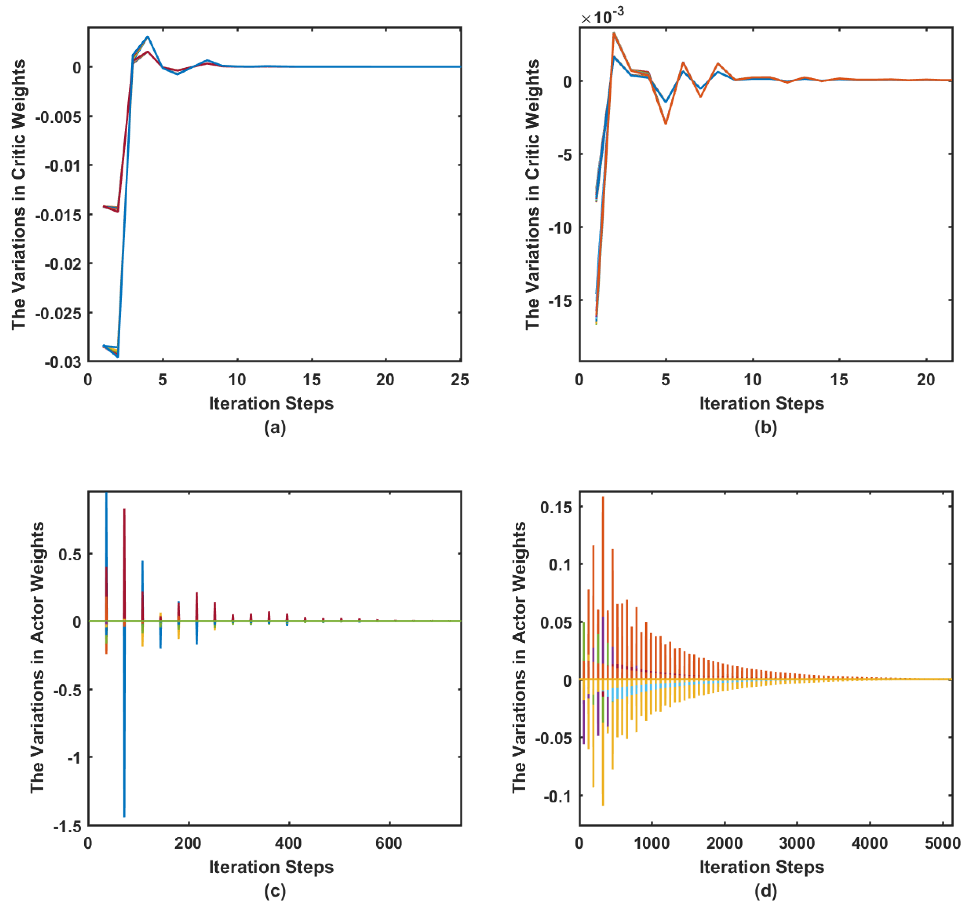
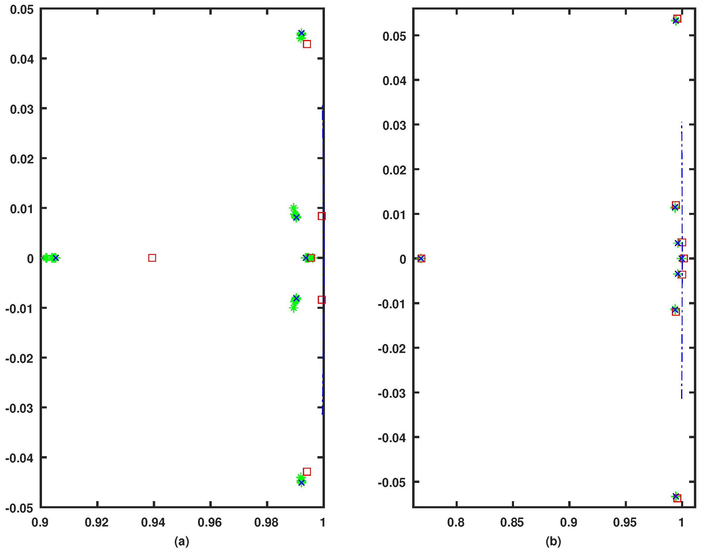
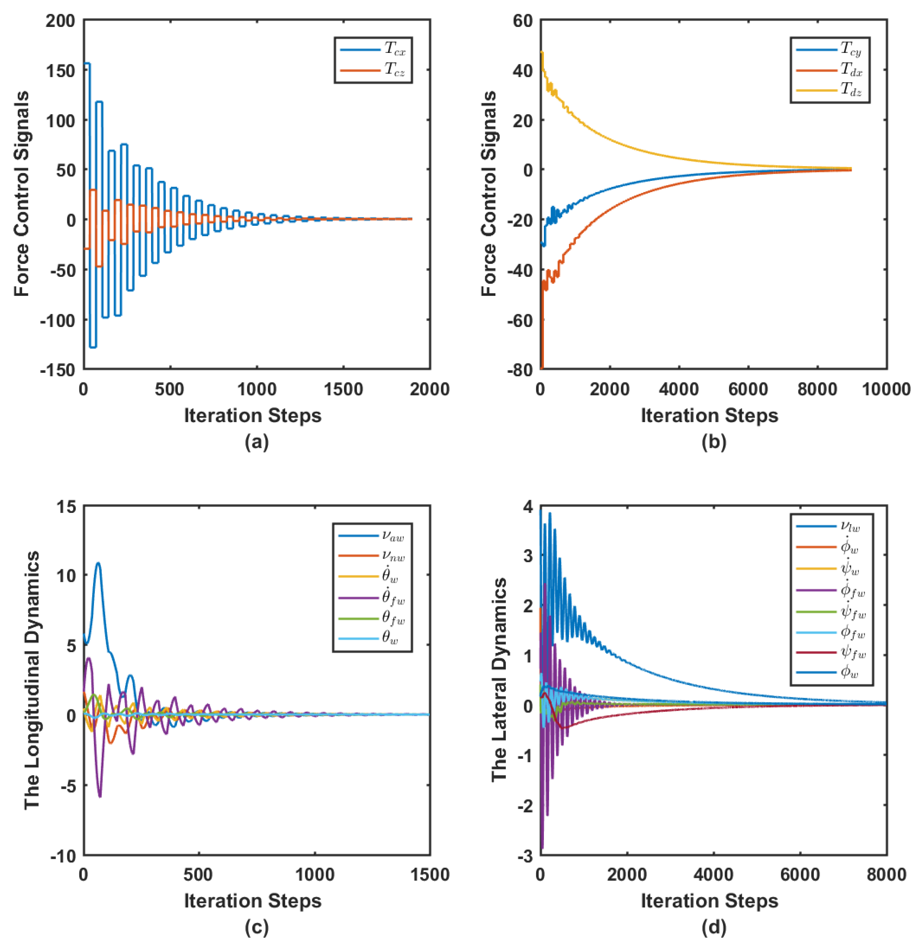
7. Simulation Results

A flexible wing hang glider is used to validate the developed model-free online adaptive learning approach [9]. The continuously varying dynamics of the flexible wing system poses a challenging control problem. This means that the controller operates in a highly uncertain dynamical environment.
The simulation results highlight the stability properties achieved by the controller in addition to monitoring its robustness against the disturbances and the dynamics’ uncertainties. Two simulation scenarios are considered: Case I shows the controller’s performance in nominal conditions (i.e., at a certain trim speed), while Case II tests the robustness of the developed controller by comparing its performance to the classical Riccati control approach under various disturbances.

7.1. Simulation Parameters

The longitudinal and lateral state space matrices of the flexible wing system, A L o , B L o , A L a , and B L a , at a given trim speed, are used to generate the online measurements [9].
The actor and critic learning parameters are set to η a = η c = 0 . 001 . The weight matrices for the longitudinal ( R L o , Q L o ) and lateral ( R L a , Q L a ) directions are taken as
R L o = 10 4 × [ 0.1000 0.4000 ] , Q L o [ 0.0100 0.0400 0.1013 0.1013 0.4053 0.4053 ] , R L a = 10 4 × [ 0.0250 0.1000 0.4000 ] , Q L a [ 0.0400 0.1013 0.1013 0.1013 0.1013 0.4053 0.4053 0.4053 ] .
The eigenvalue structures of the simulated case studies are given the following graphical notations. The open-loop eigenvalues are denoted by . The * refer to the closed-loop eigenvalues during the learning process. The eigenvalues resulting from the model-free approach are symbolized by ×. The eigenvalues evaluated by the Riccati solution are shown as .

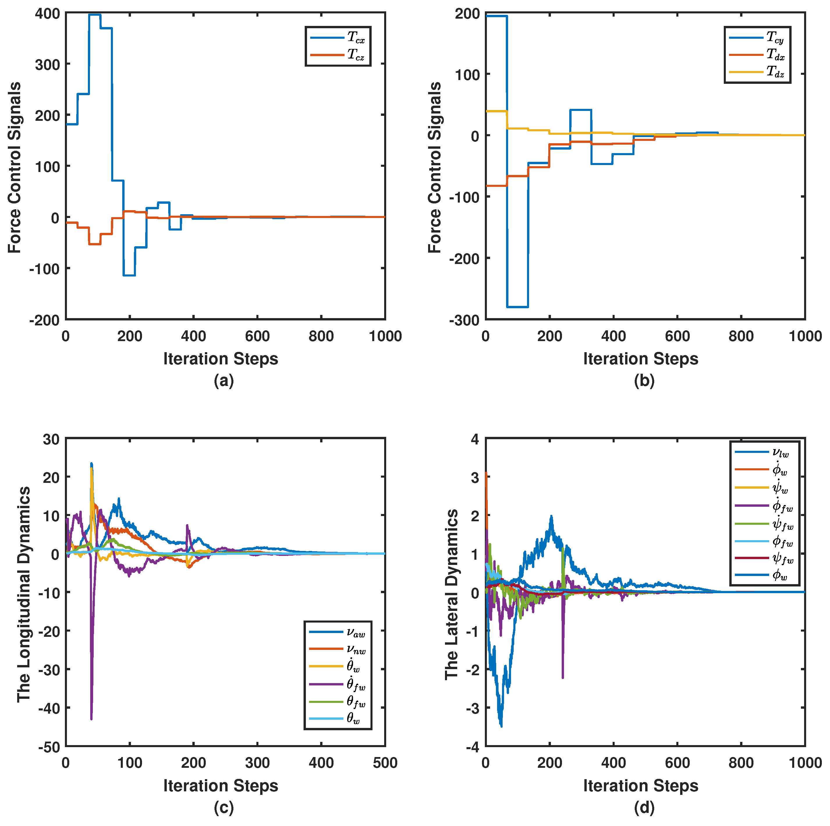
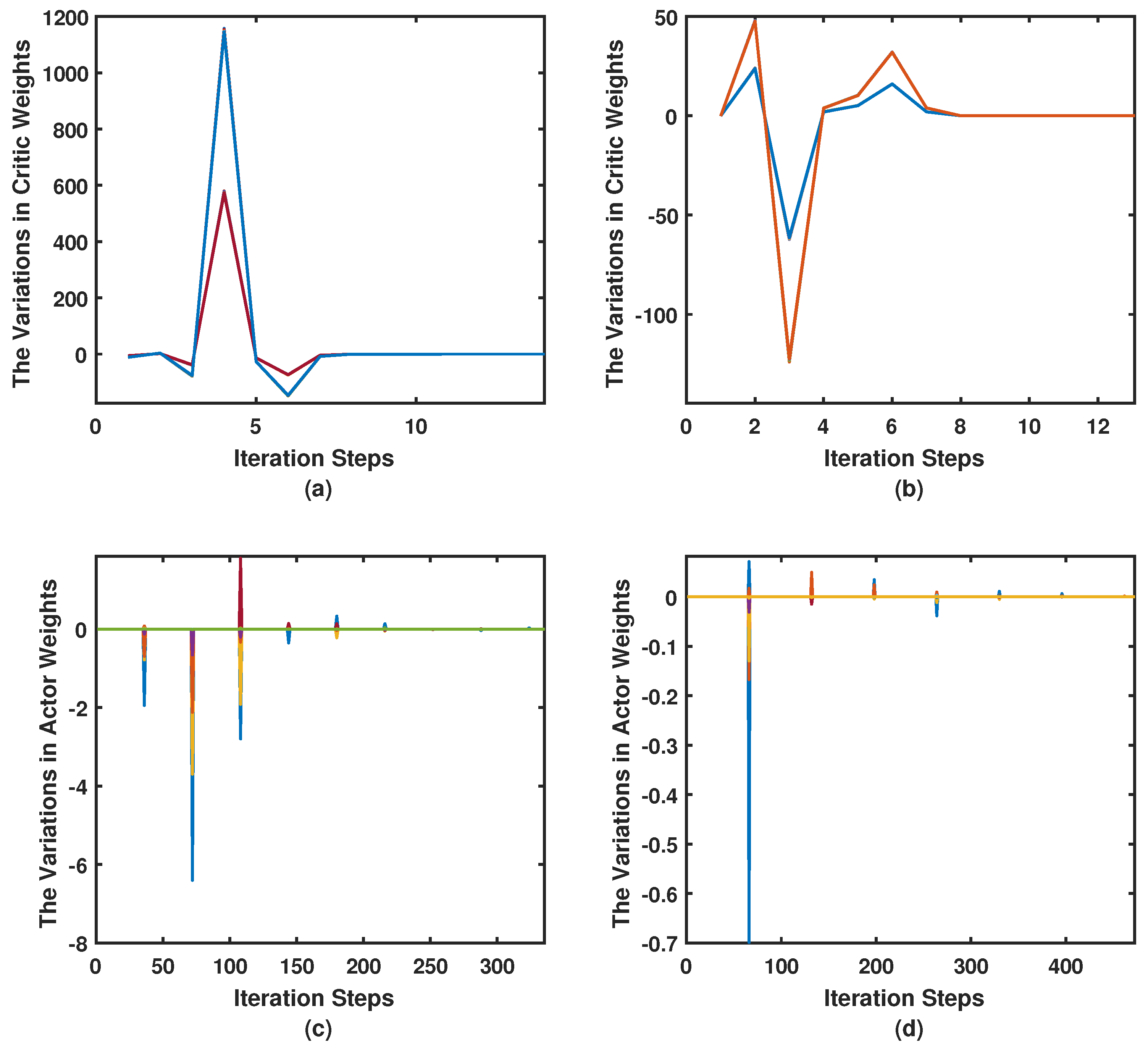
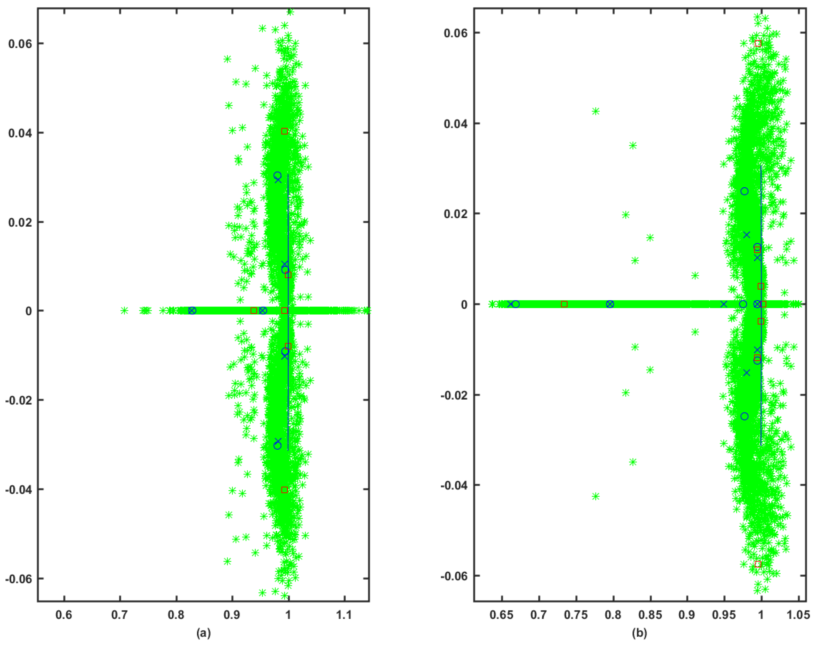
7.2. Simulation Case I

This case shows the simulation outcome when the adaptive learning algorithm is applied to control the decoupled longitudinal and lateral dynamical systems in real-time. The open- and closed-loop poles are tabulated in Table 1. The online controller was able to asymptotically stabilize the longitudinal and lateral open-loop systems. The dominant modes are damped much faster than the open-loop system, as shown by the eigenvalue structures in Figure 2. This is further emphasized by Figure 3,
The state space matrices for the longitudinal decoupled dynamics A L o and B L o are
A L o = [ 0.9906 0.0272 0.0982 0.0006 0.1400 0.0927 0.0065 0.9828 0.0737 0.0002 0.0504 0.0312 0.0018 0.0084 0.9501 0.0000 0.0018 0.0002 0.0057 0.0024 0.0990 0.9990 0.1735 0.0002 0.0000 0.0000 0.0005 0.0100 0.9991 0.0000 0.0000 0.0000 0.0097 0.0000 0.0000 1.0000 ] ,
B L o = [ 0.0004 0.0002 0.0002 0.0001 0.0005 0.0002 0.0011 0.0005 0.0000 0.0000 0.0000 0.0000 ] .
The state space matrices for the lateral decoupled dynamics A L a and B L a are
A L a = [ 0.9923 0.0437 0.0939 0.0012 0.0000 0.2393 0.0806 0.0924 0.0150 0.7661 0.0816 0.0000 0.0000 0.0019 0.0003 0.0007 0.0009 0.0009 0.9949 0.0000 0.0000 0.0011 0.0004 0.0000 0.0078 0.2202 0.0748 0.9985 0.0000 0.2791 0.0937 0.0004 0.0060 0.0796 0.0328 0.0000 1.0000 0.0027 0.0004 0.0003 0.0001 0.0013 0.0005 0.0100 0.0037 0.9986 0.0005 0.0000 0.0000 0.0004 0.0002 0.0000 0.0106 0.0000 1.0000 0.0000 0.0001 0.0088 0.0038 0.0000 0.0000 0.0000 0.0000 1.0000 ] ,
B L a = [ 0.0008 0.0000 0.0002 0.0002 0.0000 0.0000 0.0000 0.0000 0.0000 0.0010 0.0000 0.0002 0.0006 0.0003 0.0000 0.0000 0.0000 0.0000 0.0000 0.0000 0.0000 0.0000 0.0000 0.0000 ] .
where the dynamics and the input force control signals are shown to be stable. The adaption process of the actor and the critic neural network weights for both motion frames are shown in Figure 4. The plots demonstrate the converging behavior of the controller. Note that the weights appear in groups as they are too close to show individually. The actor weights are updated after ( n + m ) × ( n + m + 1 ) / 2 steps.

7.3. Simulation Case II

This case tests the robustness of the online reinforcement learning algorithm against the uncertainties in the dynamic environment of the flexible wing system (i.e., the matrices A L o / L a and B L o / L a ) on top of the disturbances in the longitudinal and lateral states δ L o / L a . The dynamic uncertainties and disturbances in the states are sampled from a normal Gaussian distribution with amplitudes of up to ± 50 % and ± 20 % of the nominal values, respectively. This scenario combines the Riccati classical control technique and the developed online adaptive learning approach such that
δ k + 1 = ( A + A ˜ k ) ( δ k + δ ˜ k ) + B u k R i c + ( B ˜ B ) u k R L .
where A ˜ k and B ˜ k are the real-time uncertainties in the drift dynamics A and the control input matrices B. The terms u k R i c and u k R L are the control input signals calculated by the Riccati and the online reinforcement learning approaches, respectively.
The eigenvalue structures in Table 2 reveal that the disturbed open-loop systems are unstable. However, the combined approach was able to asymptotically stabilize them. Furthermore, it is able to provide faster longitudinal and lateral dominant modes compared to those obtained by the Riccati solution. This is further emphasized by the dynamics and the force control signals shown in Figure 5. The comparison between the eigenvalue structures obtained in Table 1 and Table 2 reveals that the combined approach resulted in faster response compared to the Riccati solution and the original response of the longitudinal and the lateral systems. The convergence behavior of the actor-critic weights is shown in Figure 6, where the adaptation of the weights takes longer this time due to the higher complexity of the problem in hand. The eigenvalues evolution during the learning process is shown in Figure 7. The eigenvalues eventually converge to a stable region.

8. Conclusions

A novel online policy iteration process is developed to generalize model-free gradient based solutions for optimal control problems. The approach is considered a sub-class of the classical action dependent dual heuristic dynamic programming. The mathematical layout showed the duality between the Hamilton–Jacobi–Bellman formulation and the underlying model-free Bellman’s optimality setup. Unlike traditional costate-based solutions, the suggested method does not depend on the system’s dynamics. A Riccati solution is developed and is shown to be equivalent to solving the Bellman’s optimality equation. Artificial neural network-based approximations are employed to provide a real-time implementation of the policy iteration solution. This is accomplished using separate neural network structures to approximate the optimal strategy and the associated gradient of the solving value function. The performance of the proposed control scheme is demonstrated on a flexible wing aircraft. The simulation scenarios proved the effectiveness of the proposed controller under a wide range of uncertainties and disturbances in the system dynamics.

Author Contributions

This article is an outcome of the research primarily conducted by M.A. He conceived, designed, and performed the experiments. He also wrote most of the paper. W.G. supervised and directed the research. He also helped analyze the results and contributed in writing and editing the article. F.L. played an advisory role.

Funding

This research was partially funded by Ontario Centres of Excellence (OCE).

Conflicts of Interest

The authors declare no conflict of interest. The funding sponsors had no role in the design of the study; in the collection, analyses, or interpretation of data; in the writing of the manuscript, and in the decision to publish the results.

Abbreviations

The following abbreviations are used in this manuscript:
Variables
ν a w , ν l w , ν n w Axial, lateral, and normal velocities in the wing’s frame of motion.
θ w , ϕ w , ψ w Pitch, roll, and yaw angles in the wing’s frame of motion.
θ ˙ w , ϕ ˙ w , ψ ˙ w Pitch, roll, and yaw angle rates in the wing’s frame of motion.
θ f w , ϕ f w , ψ f w Pitch, roll, and yaw angles of the fuselage relative to the wing’s frame of motion.
θ ˙ f w , ϕ ˙ f w , ψ ˙ f w Pitch, roll, and yaw angle rates of the fuselage relative to the wing’s frame of motion.
T R , L Right and left internal forces on the control bar.
Subscripts
( · ) x , y , z X, Y, and Z Cartesian components of ( · ) , respectively.
Abbreviations
ADPAdaptive Dynamic Programming
ADDHPAction Dependent Dual Heuristic Dynamic Programming
DHPDual Heuristic Dynamic Programming
HJBHamilton–Jacobi–Bellman
RLReinforcement Learning

References

  1. Bertsekas, D.; Tsitsiklis, J. Neuro-Dynamic Programming, 1st ed.; Athena Scientific: Belmont, MA, USA, 1996. [Google Scholar]
  2. Werbos, P. Beyond Regression: New Tools for Prediction and Analysis in the Behavior Sciences. Ph.D. Thesis, Harvard University, Cambridge, MA, USA, 1974. [Google Scholar]
  3. Werbos, P. Neural Networks for Control and System Identification. In Proceedings of the 28th Conference on Decision and Control, Tampa, FL, USA, 13–15 December 1989; pp. 260–265. [Google Scholar]
  4. Miller, W.T.; Sutton, R.S.; Werbos, P.J. Neural Networks for Control: A Menu of Designs for Reinforcement Learning Over Time, 1st ed.; MIT Press: Cambridge, MA, USA, 1990; pp. 67–95. [Google Scholar]
  5. Werbos, P. Approximate Dynamic Programming for Real-time Control and Neural Modeling. In Handbook of Intelligent Control: Neural, Fuzzy, and Adaptive Approaches; Chapter 13; White, D.A., Sofge, D.A., Eds.; Van Nostrand Reinhold: New York, NY, USA, 1992. [Google Scholar]
  6. Howard, R.A. Dynamic Programming and Markov Processes; Four Volumes; MIT Press: Cambridge, MA, USA, 1960. [Google Scholar]
  7. Abouheaf, M.; Lewis, F. Dynamic Graphical Games: Online Adaptive Learning Solutions Using Approximate Dynamic Programming. In Frontiers of Intelligent Control and Information Processing; Chapter 1; Liu, D., Alippi, C., Zhao, D., Zhang, H., Eds.; World Scientific: Singapore, 2014; pp. 1–48. [Google Scholar]
  8. Blake, D. Modelling The Aerodynamics, Stability and Control of The Hang Glider. Master’s Thesis, Centre for Aeronautics—Cranfield University, Silsoe, UK, 1991. [Google Scholar]
  9. Cook, M.; Spottiswoode, M. Modelling the Flight Dynamics of the Hang Glider. Aeronaut. J. 2005, 109, I–XX. [Google Scholar] [CrossRef]
  10. Cook, M.V.; Kilkenny, E.A. An experimental investigation of the aerodynamics of the hang glider. In Proceedings of the an International Conference on Aerodynamics, London, UK, 15–18 October 1986. [Google Scholar]
  11. De Matteis, G. Response of Hang Gliders to Control. Aeronaut. J. 1990, 94, 289–294. [Google Scholar] [CrossRef]
  12. de Matteis, G. Dynamics of Hang Gliders. J. Guid Control Dyn. 1991, 14, 1145–1152. [Google Scholar] [CrossRef]
  13. Kilkenny, E.A. An Evaluation of a Mobile Aerodynamic Test Facility for Hang Glider Wings; Technical Report 8330; College of Aeronautics, Cranfield Institute of Technology: Cranfield, UK, 1983. [Google Scholar]
  14. Kilkenny, E. Full Scale Wind Tunnel Tests on Hang Glider Pilots; Technical Report; Cranfield Institute of Technology, College of Aeronautics, Department of Aerodynamics: Cranfield, UK, 1984. [Google Scholar]
  15. Kilkenny, E.A. An Experimental Study of the Longitudinal Aerodynamic and Static Stability Characteristics of Hang Gliders. Ph.D. Thesis, Cranfield University, Silsoe, UK, 1986. [Google Scholar]
  16. Vrancx, P.; Verbeeck, K.; Nowe, A. Decentralized Learning in Markov Games. IEEE Trans. Syst. Man Cybern. Part B 2008, 38, 976–981. [Google Scholar]
  17. Webros, P.J. A Menu of Designs for Reinforcement Learning over Time. In Neural Networks for Control; Miller, W.T., III, Sutton, R.S., Werbos, P.J., Eds.; MIT Press: Cambridge, MA, USA, 1990; pp. 67–95. [Google Scholar]
  18. Sutton, R.S.; Barto, A.G. Reinforcement Learning: An Introduction, 2nd ed.; MIT Press: Cambridge, MA, USA, 1998. [Google Scholar]
  19. Si, J.; Barto, A.; Powell, W.; Wunsch, D. Handbook of Learning and Approximate Dynamic Programming; The Institute of Electrical and Electronics Engineers, Inc.: New York, NY, USA, 2004. [Google Scholar]
  20. Prokhorov, D.; Wunsch, D. Adaptive Critic Designs. IEEE Trans. Neural Netw. 1997, 8, 997–1007. [Google Scholar]
  21. Abouheaf, M.; Lewis, F.; Vamvoudakis, K.; Haesaert, S.; Babuska, R. Multi-Agent Discrete-Time Graphical Games And Reinforcement Learning Solutions. Automatica 2014, 50, 3038–3053. [Google Scholar]
  22. Lewis, F.; Vrabie, D.; Syrmos, V. Optimal Control, 3rd ed.; John Wiley: New York, NY, USA, 2012. [Google Scholar]
  23. Bellman, R. Dynamic Programming; Princeton University Press: Princeton, NJ, USA, 1957. [Google Scholar]
  24. Abouheaf, M.; Lewis, F. Approximate Dynamic Programming Solutions of Multi-Agent Graphical Games Using Actor-critic Network Structures. In Proceedings of the International Joint Conference on Neural Networks (IJCNN), Dallas, TX, USA, 4–9 August 2013; pp. 1–8. [Google Scholar]
  25. Abouheaf, M.; Lewis, F.; Mahmoud, M.; Mikulski, D. Discrete-time Dynamic Graphical Games: Model-free Reinforcement Learning Solution. Control Theory Technol. 2015, 13, 55–69. [Google Scholar]
  26. Abouheaf, M.; Gueaieb, W. Multi-Agent Reinforcement Learning Approach Based on Reduced Value Function Approximations. In Proceedings of the IEEE International Symposium on Robotics and Intelligent Sensors (IRIS), Ottawa, ON, Canada, 5–7 October 2017; pp. 111–116. [Google Scholar]
  27. Widrow, B.; Gupta, N.K.; Maitra, S. Punish/reward: Learning with a Critic in Adaptive Threshold Systems. IEEE Trans. Syst. Man Cybern. 1973, SMC-3, 455–465. [Google Scholar] [CrossRef]
  28. Webros, P.J. Neurocontrol and Supervised Learning: An Overview and Evaluation. In Handbook of Intelligent Control: Neural, Fuzzy, and Adaptive Approaches; White, D.A., Sofge, D.A., Eds.; Van Nostrand Reinhold: New York, NY, USA, 1992; pp. 65–89. [Google Scholar]
  29. Busoniu, L.; Babuska, R.; Schutter, B.D. A Comprehensive Survey of Multi-Agent Reinforcement Learning. IEEE Trans. Syst. Man Cybern. Part C 2008, 38, 156–172. [Google Scholar]
  30. Abouheaf, M.; Mahmoud, M. Policy Iteration and Coupled Riccati Solutions for Dynamic Graphical Games. Int. J. Digit. Signals Smart Syst. 2017, 1, 143–162. [Google Scholar]
  31. Lewis, F.L.; Vrabie, D. Reinforcement learning and adaptive dynamic programming for feedback control. IEEE Circuits Syst. Mag. 2009, 9, 32–50. [Google Scholar]
  32. Vrabie, D.; Lewis, F.; Pastravanu, O.; Abu-Khalaf, M. Adaptive Optimal Control for Continuous-Time Linear Systems Based on Policy Iteration. Automatica 2009, 45, 477–484. [Google Scholar]
  33. Abouheaf, M.I.; Lewis, F.L.; Mahmoud, M.S. Differential graphical games: Policy iteration solutions and coupled Riccati formulation. In Proceedings of the 2014 European Control Conference (ECC), Strasbourg, France, 24–27 June 2014; pp. 1594–1599. [Google Scholar]
  34. Asma Al-Tamimi, F.L.L.; Abu-Khalaf, M. Model-Free Q-Learning Designs for Linear Discrete-Time Zero-Sum Games with Application to H-infinity Control. Automatica 2007, 43, 473–481. [Google Scholar]
  35. Bahare Kiumarsi, F.L.L. Actor–Critic-Based Optimal Tracking for Partially Unknown Nonlinear Discrete-Time Systems. IEEE Trans. Neural Netw. Learn. Syst. 2105, 26, 140–151. [Google Scholar]
  36. Kiumarsi, B.; Vamvoudakis, K.G.; Modares, H.; Lewis, F.L. Optimal and Autonomous Control Using Reinforcement Learning: A Survey. IEEE Trans. Neural Netw. Learn. Syst. 2018, 29, 2042–2062. [Google Scholar]
  37. Cook, M.V. The Theory of the Longitudinal Static Stability of the Hang-glider. Aeronaut. J. 1994, 98, 292–304. [Google Scholar] [CrossRef]
  38. Ochi, Y. Modeling of the Longitudinal Dynamics of a Hang Glider. In Proceedings of the AIAA Modeling and Simulation Technologies Conference, American Institute of Aeronautics and Astronautics, Kissimmee, FL, USA, 5–9 January 2015; pp. 1591–1608. [Google Scholar]
  39. Ochi, Y. Modeling of Flight Dynamics and Pilot’s Handling of a Hang Glider. In Proceedings of the AIAA Modeling and Simulation Technologies Conference, American Institute of Aeronautics and Astronautics, Grapevine, TX, USA, 9–13 January 2017; pp. 1758–1776. [Google Scholar]
  40. Sweeting, J. An Experimental Investigation of Hang Glider Stability. Master’s Thesis, College of Aeronautics, Cranfield University, Silsoe, UK, 1981. [Google Scholar]
  41. Cook, M. Flight Dynamics Principles; Butterworth-Heinemann: London, UK, 2012. [Google Scholar]
  42. Kroo, I. Aerodynamics, Aeroelasticity and Stability of Hang Gliders; Stanford University: Stanford, CA, USA, 1983. [Google Scholar]
  43. Spottiswoode, M. A Theoretical Study of the Lateral-directional Dynamics, Stability and Control of the Hang Glider. Master’s Thesis, College of Aeronautics, Cranfield Institute of Technology, Cranfield, UK, 2001. [Google Scholar]
  44. Cook, M.V. (Ed.) Flight Dynamics Principles: A Linear Systems Approach to Aircraft Stability and Control, 3rd ed.; Aerospace Engineering; Butterworth-Heinemann: Oxford, UK, 2013. [Google Scholar]
Figure 1. A flexible wing hang glider.
Robotics 07 00066 g001
Figure 2. Case I. The eigenvalue structures during the learning process: (a) the longitudinal system; and (b) the lateral system.
Robotics 07 00066 g002
Figure 3. Case I. The longitudinal and lateral force control signals and the dynamics: (a) the longitudinal force control signals; (b) the lateral force control signals; (c) the longitudinal dynamics; and (d) the lateral dynamics.
Robotics 07 00066 g003
Figure 4. Case I. The variations in the neural networks’ weights: (a) the variations in the actor’s weights for the longitudinal case; (b) the variations in the actor’s weights for the lateral case; (c) the variations in the critic’s weights for the longitudinal case; and (d) the variations in the critic’s weights for the lateral case.
Robotics 07 00066 g004
Figure 5. Case II. The longitudinal and lateral force control signals and the dynamics: (a) the longitudinal force control signals; (b) the lateral force control signals; (c) the longitudinal dynamics; and (d) the lateral dynamics.
Robotics 07 00066 g005
Figure 6. Case II. The variations in the neural networks’ weights: (a) the variations in the actor’s weights for the longitudinal case; (b) the variations in the actor’s weights for the lateral case; (c) the variations in the critic’s weights for the longitudinal case; and (d) the variations in the critic’s weights for the lateral case.
Robotics 07 00066 g006
Figure 7. Case II. The eigenvalue structures during the learning process: (a) the longitudinal system; and (b) the lateral system.
Robotics 07 00066 g007
Table 1. Open and closed-loop eigenvalues (Case I).
Longitudinal Dynamics
Open-Loop System 0.9394 , 0.9950 e ± 0.0431
0.9954 , 0.9994 e ± 0.0084
Closed-Loop system 0.9053 , 0.9904 e ± 0.0082
0.9932 e ± 0.0454 , 0.9937
Lateral Dynamics
Open-Loop System 0.7687 , 0.9945 e ± 0.0120
0.9971 e ± 0.0539
1.0000 e ± 0.0036 , 1.0016
Closed-Loop system 0.7684 , 0.9937 e ± 0.0116
0.9957 e ± 0.0535
0.9961 e ± 0.0035 , 0.9995
Table 2. Open and closed-loop eigenvalues (Case II).
Longitudinal Dynamics
Open-Loop System 0.9387 , 0.9938 , 0.9940 e ± 0.0404
(Disturbed System) 1.0002 e ± 0.0080
Closed-Loop System 0.8289 , 0.9551 , 0.9818 e ± 0.0308
(Riccati Solution) 0.9953 e ± 0.0092
Closed-Loop System 0.8271 , 0.9533 , 0.9824 e ± 0.0298
(Model-Free Solution) 0.9932 e ± 0.0104
Lateral Dynamics
Open-Loop System
(Disturbed System)
0.7346 , 0.9972 e ± 0.0578 0.9948 e ± 0.0121 , 0.9996 e ± 0.0038 , 1.0021
Open-Loop System
(Riccati Solution)
0.6685 , 0.7963 , 0.9778 e ± 0.0254 0.9944 e ± 0.0126 0.9750 , 0.9945
Closed-Loop system
(Model-Free Solution)
0.6622 , 0.7956 , 0.9492 0.9799 e ± 0.0156 , 0.9942 e ± 0.0102 0.9942

