1. Introduction
In the last 20 years, the field of autonomous robotics has grown a lot because of new developments in sensing, computing, and artificial intelligence. The ability to plan and find ways to avoid collisions in complicated environments is what makes any autonomous robot work. Path planning is the most important part of autonomous navigation systems. This includes delivery robots moving through hospital halls, self-driving cars driving through city traffic, and unmanned aerial vehicles (UAVs) searching and rescuing. Path-planning algorithms could be broadly categorized into general (graph-based and grid-based) algorithms, sampling-based algorithms, and reactive algorithms. Each type of algorithm has its own advantages and limitations. Traditional methods (such as A*) give optimal solutions for discrete static environments and cannot deal with dynamic motion. Sampling-based methods such as RRT* and PRM* may be used to solve problems in high-dimensional configuration space, but may be slow. Reactive methods such as Potential Fields can respond in real time, but may become stuck in local minima. Path planning for robots in a dynamic environment is one of the most interesting yet least researched issues in real-world robotics. Unlike controlled lab environments, the real world is dynamic: people are walking, doors are opening and closing, at any moment you can find a new construction site, and sensor readings vary. A robot not only has to plan its path, but it must also perceive the environment around it and replan its path accordingly. This means there needs to be a strong link between perception (environment awareness) and planning—we call it environment-to-robot awareness. The key contributions of this work are as follows:
An extension of the classical potential field method (APF) with dynamic effects of obstacle velocity and directional influence (APF-D).
A comparative analysis of the classical and modern algorithms of path planning in the circumstances of dynamics.
A world-wide approach with domestic responsiveness flexibility.
Motivation
The majority of comparative studies of path-planning algorithms have concentrated solely on static environments, and the dynamic replanning issue has thus far not been addressed in comparative studies. This poses a very big disparity between school standards and practical implementation needs. We are driven by the following observations in our study:
The performance degradation of classical algorithms in dynamic environments is not reflected by benchmarks using static environments.
There is no extensive comparison that evaluates all major families of algorithms within the same dynamic environment.
Environment-awareness mechanisms are seldom considered as a performance metric, even though they are essential for real-life implementation.
Literature on hybrid methods that use several algorithmic approaches is not thoroughly developed.
2. Literature Review
Compared to the existing literature, this paper offers a single assessment system and emphasizes the significance of environment-conscious replanning in dynamic robots. Comparative studies of classical and intelligent path-planning techniques for autonomous mobile robots have been conducted previously [
1].
2.1. Global Path-Planning Methods
Global and local (reactive) planning algorithms are the two main categories for path-planning algorithms used in autonomous mobile robots. Approaches to global path planning have the assumption that the robot already possesses some information regarding the environment in which it operates. In this approach, an optimal path for collision-free movement is determined beforehand based on optimization of the objective functions, such as distance traveled, time taken, or cost of the path. Though these approaches produce highly accurate results, they suffer when rapid changes occur frequently in the environment [
2,
3,
4,
5]. It has been found in recent research that reliable and collision-free navigation is possible through global path planning when an exact environment map is used [
4]. However, the repeated recomputation of the global path limits their applicability in rapidly changing environments, motivating the development of adaptive planning strategies. Some examples of global planning algorithms include graph-searching algorithms such as A*, D*, D* lite, and Dijkstra; and also some sampling-based algorithms like PRM and RRT* [
6,
7,
8,
9,
10,
11].
Advantages:Global planning algorithms generate complete and sometimes optimal solutions, hence, their effectiveness in static environments with an accurate map [
2,
3].
Disadvantages: The performance of global planning algorithms degrades in dynamic environments due to the necessity of constant replanning as a result of any change in the environment, which causes more computational overhead and less real-time response [
3,
8,
12]. As shown in recent works, graph-based planning methods still prove to be the best approach for problems where deterministic behavior and navigation, along with path optimization, are needed, such as those encountered in warehouse logistics, autonomous transport systems, and service robotics. The problem is that their reliance on the accuracy of the map of the environment and heavy computation for repeated planning hinders their application in rapidly changing environments. For this reason, current research concentrates on combining graph searching with adaptive and environmental awareness techniques [
2,
3,
12,
13].
2.2. Classical Graph-Based Methods
Global path planning for AMRs is a very well-explored approach using classical graph-based algorithms, which are known as complete and optimal with proper heuristics [
1]. A comprehensive comparative review of graph-based, sampling-based, and reactive path-planning algorithms for autonomous robots was summarized in [
13]. The paper pointed out that although graph-search techniques are less effective in dynamic environments with frequent replanning, they are still very useful in structured environments. The method is represented as a graph where nodes are the states or grid cells that the robot can be in, and the edges are the transitions between them. The goal is to find the cost-minimum path using graph-search algorithms [
2,
3,
6] from the initial node to the goal node. One of the important graph-search algorithms is the A* algorithm formulated by Hart et al. [
6]. The evaluation function used by the A* algorithm for evaluating each candidate node is
where
is the cost of reaching the current node from the starting node, and
is the heuristic estimation of the cost required to reach the goal node. The use of an admissible heuristic ensures that the A* algorithm finds the optimal solution by limiting the search space to a much smaller one than the uninformed search techniques. Some improved versions, such as Weighted A*, Anytime Repairing A* (ARA*), and Incremental A*, are available. The hybrid A* algorithm has also been used for autonomous mobile robots by integrating graph-based planning algorithms along with the kinematic constraints of the vehicles [
14]. The D* (Dynamic A*) algorithm was presented by [
7] to deal with navigation within a partially known and dynamic environment by updating the earlier calculated path rather than doing complete replanning in case of any changes in the environment [
7]. The D* Lite algorithm is an improvement of D* and provides the same capability of replanning with the advantage of less complexity and computational cost [
8]. This algorithm updates the affected parts of the search graph and therefore reduces the time required for replanning and becomes one of the most used graph algorithms for dynamic robot navigation [
3,
12]. More experimental results on the comparison between A* and D* Lite show that D* Lite is much faster in adapting itself for replanning in dynamic grids because of its incremental search strategy [
15]. Eexperimentally comparing A and D Lite in dynamic navigation scenarios shows that D* Lite significantly reduces replanning time by updating only the affected regions of the search graph instead of recomputing the complete path. This incremental search strategy enables efficient real-time navigation under changing environmental conditions [
15].
Advantages: Graph-based techniques create an entire and perfect path for navigation when heuristic functions are used. The methods deliver a predictable and consistent trajectory, a deterministic solution, and good efficiency in structured settings where there are exact environmental maps available. It makes the method a good choice for warehouse automation, indoor robots, and autonomous cars that move around in static environments [
2,
3].
Weaknesses: Although these algorithms work well, their computation cost rises with the increase in the size of the map and the number of obstacles. Additionally, if the surroundings keep changing, there is always a need for replanning, thus increasing the computation cost. Therefore, these algorithms are inefficient in dynamic or unknown environments, hence calling for the development of environment-aware navigation techniques that can respond quickly to changes in obstacles [
8,
12,
13].
2.3. Sampling-Based Methods
In other words, sampling-based methods of trajectory generation generate robot-feasible trajectories through the random sampling of the robot configuration space, instead of performing the full search on a discretized graph. Sampling-based methods can thus easily deal with high-dimensional configuration spaces and complex robot kinematics, while only requiring a modest amount of knowledge regarding the environment [
2,
3].
Among the early sampling-based algorithms, we may mention the work of [
9], namely Probabilistic Roadmap (PRM) [
9]. PRM decomposes the process of trajectory generation into two stages. First, during the offline learning stage, collision-free configurations are randomly generated and then connected to form a roadmap. Then, during the online query stage, the start and goal configurations are connected to the roadmap to form a feasible path. Ref. [
11] enhanced the algorithm by proposing PRM* with guaranteed asymptotic optimality.
Another sampling-based algorithm is the Rapidly Exploring Random Tree (RRT) algorithm proposed by [
10,
16]. The RRT method builds a search tree starting from the initial configuration using random samples from the configuration space, and it is especially suitable for dealing with motion planning in high-dimensional and non-holonomic spaces. In addition to this, ref. [
11] have introduced RRT* by incorporating a rewiring process to the algorithm in order to reach asymptotic optimality while retaining the exploration feature of RRT. Various modifications, such as Informed RRT* and BIT*, have been made in order to increase the rate of convergence. Recent advancements like Bi-AM-RRT* improve sampling efficiency and convergence rate through bidirectional tree growth and adaptive motion planning techniques, and hence are appropriate for dynamic situations as well [
17]. Another area where studies have been conducted involves the development of a fast-revisit coverage path plan with the help of long-range sensor data for patrolling robots [
16].
Advantages: Sampling-based planning methods effectively solve the problems of motion planning in high-dimensional space without the necessity to discretize the environment completely. These methods naturally account for the kinematics of the robot and non-holonomic constraints while offering significant flexibility to autonomous vehicles and manipulators moving in complicated environments [
2,
3].
Drawbacks: While being flexible, sampling-based planning algorithms produce non-smooth paths that need further processing before execution. The computational complexity of the algorithm depends on the number of samples generated, and repeated generation of samples in a highly dynamic environment with frequent replanning becomes inefficient. Despite being asymptotically optimal, convergence of PRM* and RRT* to the optimal path may take a lot of time and samples [
12,
18,
19]. Recent development of sampling-based motion planning includes improvements aimed at the acceleration of convergence rate and decrease of computational complexity by implementing more informed sampling and heuristic-based methods. Methods like Informed RRT* and others offer a significant decrease in unnecessary exploration while maintaining asymptotic optimality; thus, they are appropriate for high-dimensional robots. However, re-sampling in highly dynamic environments with frequent replanning is still computationally expensive [
18,
19,
20].
2.4. Reactive and Artificial Potential Field-Based Methods
Reactive navigation algorithms make navigation decisions based on sensory data collected in real time without the need for an environmental map. The main disadvantage of reactive navigation algorithms is their reliance on continuous adjustment of the robot’s trajectory based on the positions and movement of nearby obstacles, which makes them very useful for uncertain environments. In general, reactive algorithms have lower computational complexity and reaction speed and are able to produce only locally optimal results [
2,
3,
12]. to reduce local minima and oscillatory motion.The improvements reported here suggest the importance of combining environmental perception and reactive navigation for autonomous robots in dynamic environments.
Among reactive navigation algorithms, the most popular one is the Dynamic Window Approach (DWA) algorithm, proposed by [
21]. The DWA method finds the combination of translational and rotational velocities within the dynamic constraints of the robot such that progress towards the target point is maximized while avoiding collisions with obstacles. Due to its relatively high efficiency, DWA was widely used in mobile robots’ navigation. However, in complex environments, DWA may have some disadvantages, such as oscillatory behavior.
Another useful method of reactive navigation is the Velocity Obstacle (VO) method, proposed by Fiorini and Shiller [
22]. The VO method predicts the possibility of future collision through the analysis of relative velocities between the robot and moving obstacles. Then, the robot chooses a safe velocity from the collision region in order to navigate safely. Although the Velocity Obstacle method enhances the ability of obstacle avoidance greatly, the success of the method requires precise estimation of the obstacle velocities and motions.
The Bug algorithm family is another approach for reactive navigation. The representative examples of this category are Bug1, Bug2, and TangentBug algorithms, which rely on sensor information about the nearby obstacles and navigate the robot until it finds a way to reach the destination point without any obstacles. The advantages of these algorithms are simplicity and efficiency, but they tend to find non-optimal ways in complicated environments. Artificial potential field methods have been introduced by Khatib [
23]. In APF, the goal produces an attractive force, and the obstacles around it produce the repulsive force. The robot’s movement is based on the resultant vector of the artificial force, ensuring smooth and efficient navigation. Thanks to their efficiency and computational speed, the APF methods have been widely used for avoiding obstacles and performing local navigation.
Advantages: The reactive and APF methods are characterized by relatively low computational costs, quick responses, and high adaptability to unknown and changing environments. No need to create maps of the whole environment makes these methods suitable for navigation applications that involve moving obstacles [
2,
3,
17,
21].
Limitations: On the other hand, conventional APF methods show the problems of local minima, oscillatory movements around obstacles, and poor performance in highly dynamic environments. Like the APF, reactive approaches also offer only the locally optimal solutions and do not provide global path optimality [
12]. That is why researchers tend to develop new adaptive weights, motion prediction algorithms, and hybrid optimization methods [
5,
13,
20].
These advancements serve as the main driving force behind the development of the Adaptive Potential Field with Dynamic Awareness (APF-D) system that enhances the classical APF system through the inclusion of dynamic obstacle prediction, adaptive force adjustment, and environment-awareness techniques in order to ensure safe and efficient navigation in complex dynamic environments. The recent advancements in the field of reactive navigation include adaptive weightings, dynamic obstacle prediction, and environment-awareness approaches that help deal with the shortcomings associated with classical APF systems. The above advancements not only help improve obstacle avoidance but also help reduce oscillation and local minima problems. As a result, adaptive APF systems have gained much popularity in complex dynamic environments [
5,
12,
13,
20].
2.5. Summary of Existing Path-Planning Methods
According to the literature review, one could notice that there are certain advantages and disadvantages in each path-planning algorithm. The graph-based classical algorithms, including A* and D* Lite, provide optimal solution of problems given that the map of the environment is precise; however, these algorithms are relatively expensive in terms of cost when used in a dynamic environment due to continuous replanning. Sampling-based algorithms such as PRM* and RRT* solve the problem of high-dimensional motion planning with asymptotic optimality; however, these algorithms require more computational resources to converge. Reactive algorithms, including APF-based algorithms, are able to respond to changes in the environment effectively and have lower computational complexity; however, they are vulnerable to local minima and oscillations. In conclusion, no algorithm from the list of algorithms offers an optimal solution in all navigation cases. There is always at least one aspect that the current approaches need to sacrifice among the following: computational efficiency, optimality of the solution, and flexibility because of the dynamical properties of the environment. This demonstrates the necessity of the development of navigation systems that will be able to use the advantages of global planning, sampling, and reaction to obstacles. This is what drives the current comparison and the creation of the APF-D approach.
2.6. Research Gap: Dynamic Environment Awareness
Despite extensive research in the literature being carried out regarding the individual algorithms, there is still a gap in the literature: most tests are done in fixed settings, and dynamic replanning is addressed as an incidental consideration and not a design principle. Moreover, the notion of environment-to-robot awareness, i.e., the mechanism of sensing the changes in environmental conditions and conveying these changes to the planning module, is seldom formalized or benchmarked. This gap is directly addressed in our work since we develop a dynamic evaluation framework and measure the replanning performance when coupled with awareness.
3. Algorithm Descriptions and Theoretical Foundations
Environment awareness is implemented through a sensor-fusion layer that integrates LiDAR point clouds, camera depth maps, and odometry data to maintain a dynamic occupancy grid. When moving obstacles are detected, their velocities are estimated using Kalman filtering, and F_dyn is computed to steer the robot away from predicted collision zones. Local minima escape is achieved through a topological memory mechanism that detects oscillatory behavior and applies random perturbations when necessary. The estimate is fed to the dynamic repulsive force function, F_dyn, allowing the robot to determine the probable zone of collision and thus make proactive adjustments to its path instead of reactive ones. In order to address the issue of local minima encountered in traditional APF systems, a topological memory scheme is used. This scheme detects the oscillatory navigation pattern and injects random perturbations when the robot becomes stuck.
A* Algorithm
A best-first search algorithm is A, a search algorithm that discovers the shortest path of a weighted graph. It has an open list of nodes to be considered, and ranked in order of
. In each step, the node with the minimum value of f is expanded by the algorithm.A best-first search algorithm is A, a search algorithm that discovers the shortest path of a weighted graph. It has an open list of nodes to be considered, and ranked in order of
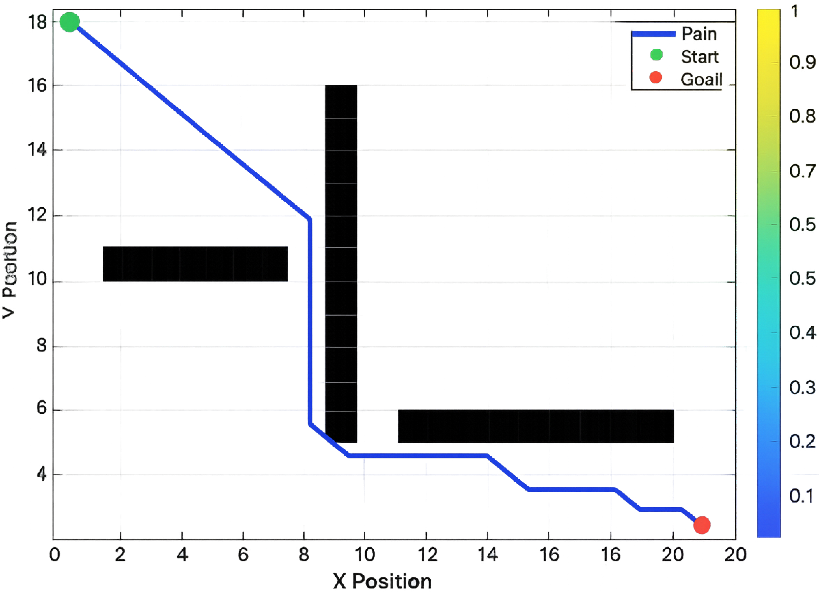
. In each step, the node with the minimum value of f is expanded by the algorithm. The black rectangles in
Figure 1 represent static structural obstacles that remain fixed throughout the simulation. The A* algorithm determines an optimal collision-free path from the start position to the goal while avoiding these obstacles. In this paper, we adopt the Euclidean distance heuristic of 2D grid worlds. Core update rule: In case a neighbor node m of the current node n is discovered at a lower path cost through n, then the g-value of that node is updated:
. The parent pointer is updated, and m is inserted into the open list and
. A* is complete and optimal in finite graphs with admissible heuristics. To do dynamic replanning, A* needs to be re-initiated each time the environment is altered, which means that it has a cost of
per replan cycle, where b is the branching factor, and d is the depth of the solution. This renders A* computationally infeasible in the highly dynamic world.
A* is a heuristic search method that uses both the real cost of traversal and the estimated distance-to-goal function to locate the best possible path through a set of nodes. The calculated path is depicted by the blue line that successfully avoids all the obstacles while keeping the optimal path. The path planner first navigates diagonally towards the target till it comes across the center obstacle, and then continues the process by following the obstacle boundary.
A* successfully calculates the path to the target in the above structured environment in an efficient manner. Although the path takes advantage of the entire environment’s prior knowledge, it still manages to navigate towards the target effectively in a low-complexity manner. However, it should be noted that A* may perform poorly in dynamic environments due to frequent requirements for path replanning. The performance of the path-planning capability of the A* algorithm in a static environment comprising various obstacles. The robot begins navigation from the initial point situated at the top-left corner to reach the target at the bottom-right corner of the environment. The detailed A* path planning algorithm is given in Algorithm 1.
| Algorithm 1 Heuristic A* Search Algorithm for Robot Navigation |
Require: Initial state , target state , workspace representation Ensure: Shortest feasible path between source and destination
- 1:
Create OPEN and CLOSED node collections - 2:
Insert starting node into OPEN set - 3:
Initialize traversal cost: - 4:
- 5:
Estimate initial evaluation function: - 6:
- 7:
while OPEN set is not empty do - 8:
Choose node with minimum evaluation value - 9:
if corresponds to target state then - 10:
Terminate search and reconstruct optimal route - 11:
end if - 12:
Remove from OPEN collection - 13:
Append to CLOSED collection - 14:
for every adjacent node connected to do - 15:
if is blocked or already explored then - 16:
Skip current neighbor - 17:
end if - 18:
Calculate temporary movement expense: - 19:
- 20:
if is unexplored OR then - 21:
Store as predecessor of - 22:
Update traversal cost: - 23:
- 24:
Evaluate heuristic estimate: - 25:
- 26:
Compute overall evaluation score: - 27:
- 28:
if is absent from OPEN collection then - 29:
Insert into OPEN collection - 30:
end if - 31:
end if - 32:
end for - 33:
end while - 34:
Report failure when no valid route exists
|
4. D* Lite Algorithm
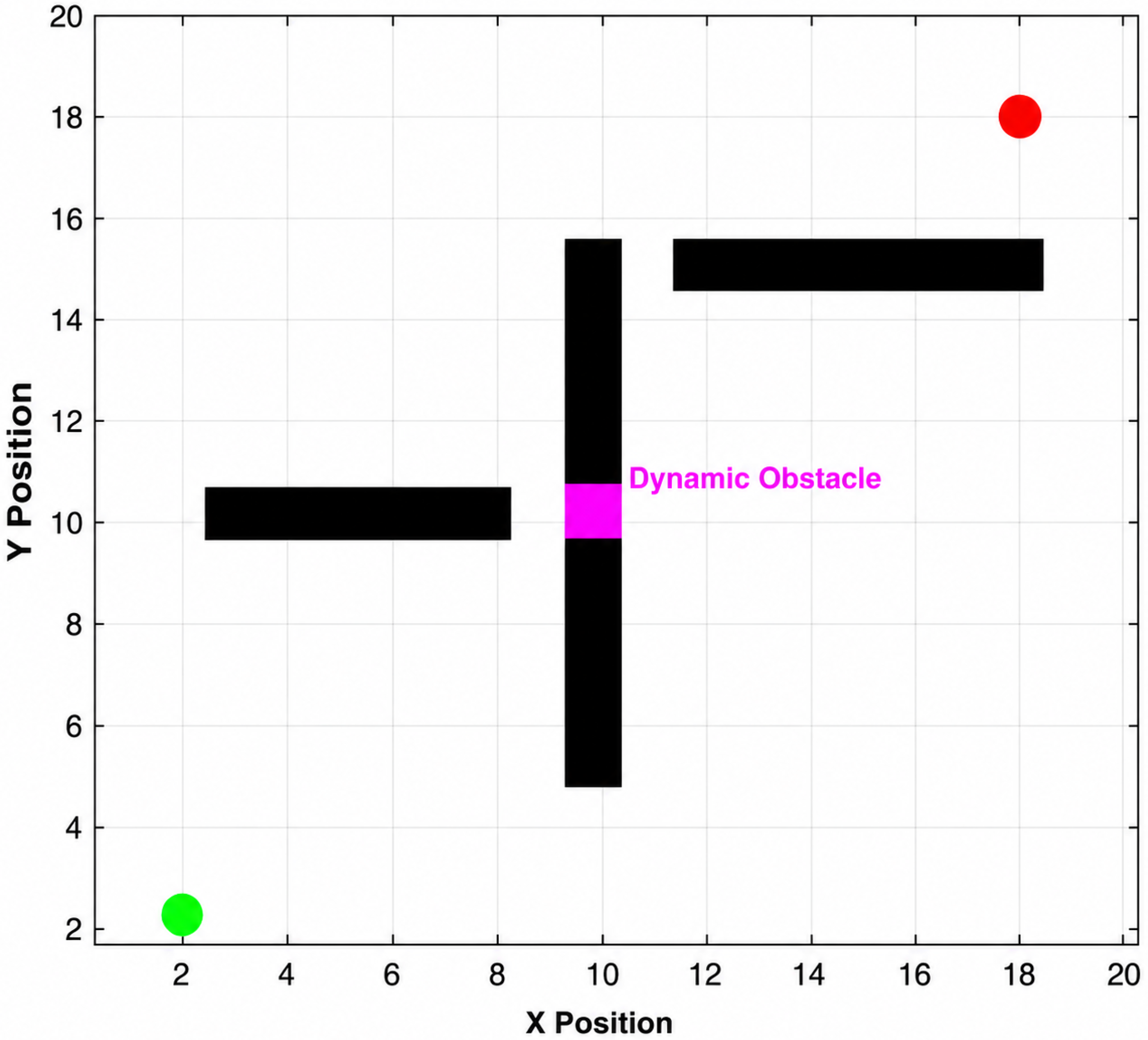
D* Lite stores an inconsistent node in a priority queue and computes them with two estimates, g(s) (cost so far to the goal) and rhs(s) (one-step lookahead). A node is locally consistent if g(s) = rhs(s). Propagation of cost updates in both directions is initiated with rhs(goal) = 0, and propagates through the algorithm. When the changes in the environment are detected, it reprocesses only the part of the search graph that is affected. The most important innovation is that the robot will move as an initial step towards the goal, and D* Lite will continue updating the plan with the current position of the robot, and only the nodes with invalidated costs will be updated. This incremental method usually involves only O(k log k) operations per replanning step, and k is the number of changed cells. The simulation results of the Adaptive D Lite algorithm in a dynamic environment are presented in
Figure 2. The black rectangular bars are static obstacles, which remain unchanged in the simulation and enforce constrained navigation corridors. The green circle is the position of the robot at the start, and the red circle is the position of the goal. The magenta rectangle represents a dynamic obstacle detected during navigation. When a dynamic obstacle is present in the planned path, the Adaptive D* Lite algorithm updates only the affected part of the path incrementally, allowing efficient replanning without any unnecessary recomputation.This allows the robot to avoid the static and dynamic obstacles safely and move towards the goal. Algorithm 2 shows the detailed D* Lite navigation algorithm.
| Algorithm 2 Adaptive D* Lite Navigation Algorithm |
Require: Initial node , destination node , dynamic workspace map Ensure: Continuously updated shortest collision-free route
- 1:
Create an empty priority queue OPEN - 2:
Initialize state values: - 3:
- 4:
Set terminal condition: - 5:
- 6:
Insert goal state into OPEN queue - 7:
while priority queue OPEN is not empty do - 8:
Select state u with minimum priority key - 9:
if then - 10:
Assign consistent value: - 11:
- 12:
for each predecessor node p connected to u do - 13:
Perform UpdateVertex(p) - 14:
end for - 15:
else - 16:
Reset node estimate: - 17:
- 18:
for all predecessor states related to u do - 19:
Execute UpdateVertex(state) - 20:
end for - 21:
end if - 22:
end while - 23:
while current robot position do - 24:
Move toward neighboring state with minimum traversal cost - 25:
if changes in environment are observed then - 26:
Modify costs of affected edges - 27:
for every impacted state do - 28:
Recalculate vertex information using UpdateVertex() - 29:
end for - 30:
Perform replanning to obtain revised shortest path - 31:
end if - 32:
end while - 33:
Output dynamically updated optimal trajectory
|
5. RRT* Algorithm
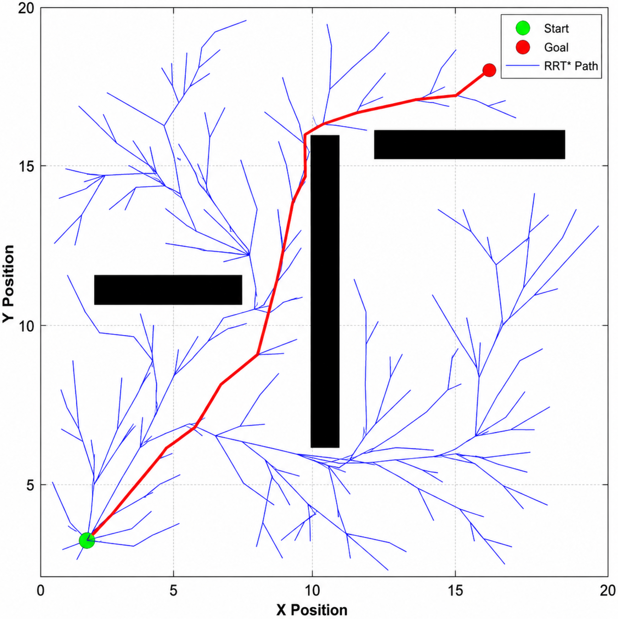
RRT* builds a tree T starting at an initial configuration qinit by repeatedly sampling random configurations qrand, locating the closest tree node qnear, extending into qrand to create qnew, and rewiring nearby nodes when a shorter path is identified via qnew. The most important change in RRT is the rewiring step, which guarantees asymptotic optimality. Connection radius r(n) = min(gamma (log(n)/n)1/d, eta) guarantees that r(n) tends towards the optimal path as n (number of samples) grows. In dynamic environments, RRT* needs to be extended with change detection and partial tree re-repairing capabilities since complete replanning is computationally costly. The Enhanced RRT* algorithm incrementally constructs a search tree by randomly sampling feasible configurations and connecting them to nearby nodes while avoiding collisions. In contrast to regular RRTs, in the case of RRT*, an effective rewiring technique is utilized, which helps improve the quality of the path found by reducing the cost of the overall travel path. The more samples are considered, the closer the resulting path reaches the asymptotically optimal one.
Figure 3 shows the enhanced RRT* path-planning simulation results. The black rectangular boxes represent static obstacles, the blue branches represent the exploration tree, and the red curve represents the optimized collision-free path from the start position (green circle) to the goal position (red circle). Based on the simulation results, the RRT* planner successfully generates a safe, collision-free path from the start position to the goal while effectively avoiding the obstacles. The detailed RRT* path-planning algorithm is presented in Algorithm 3.
| Algorithm 3 Enhanced RRT* Path-Planning Framework |
Require: Source configuration , destination configuration , workspace map Ensure: Feasible near-optimal trajectory
- 1:
Initialize search tree T using root vertex - 2:
for to N do - 3:
Produce a random sample point - 4:
Determine the closest existing vertex: - 5:
- 6:
Expand the tree toward the sampled point: - 7:
- 8:
if lies in obstacle-free space then - 9:
Identify nearby vertices within neighborhood radius r - 10:
Choose the parent node that provides minimum cumulative cost - 11:
Insert into tree structure T - 12:
for each neighboring vertex do - 13:
if updated route through reduces path expense then - 14:
Modify tree connections using rewiring operation - 15:
end if - 16:
end for - 17:
end if - 18:
if reaches the target region then - 19:
Preserve the currently best feasible solution - 20:
end if - 21:
end for - 22:
Extract the final near-optimal trajectory from to
|
5.1. PRM* Algorithm
Probabilistic Roadmap Star (PRM*) is one of the asymptotically optimal sampling-based motion planners used for high-dimensional configuration spaces. PRM* differs from graph-search algorithms that explore all grid cells explicitly because PRM* creates a probabilistic roadmap through random sampling of collision-free states and joining neighbors using a local planner. After building the roadmap, the start and goal states are added to the roadmap, and the shortest feasible path between them is found through a graph-search algorithm like Dijkstra’s algorithm. The detailed RRM* path planning algorithm is given in Algorithm 4.
| Algorithm 4 Optimized PRM* Path-Planning Procedure |
Require: Initial configuration , target configuration , occupancy map Ensure: Feasible and near-optimal navigation path
- 1:
Create an empty roadmap structure - 2:
for to N do - 3:
Randomly sample a configuration - 4:
if lies in free space then - 5:
Insert into the vertex collection V - 6:
end if - 7:
end for - 8:
for every vertex do - 9:
Determine nearby vertices inside connection radius r - 10:
for each neighboring vertex do - 11:
if local path between and is obstacle-free then - 12:
Create edge and append it to E - 13:
end if - 14:
end for - 15:
end for - 16:
Attach the start node and destination node to the roadmap - 17:
Establish valid links with closest reachable vertices - 18:
Execute graph-based optimal search to obtain final route - 19:
- 20:
Output the computed collision-free trajectory P
|
The roadmap creation procedure involves two steps. The first step involves the offline step, where free states are sampled and joined to other nodes in the graph within a certain distance called the connection radius. The second step is the online query, where the start and goal nodes are added to the roadmap and joined to their nearest feasible neighbors before finding the shortest path.
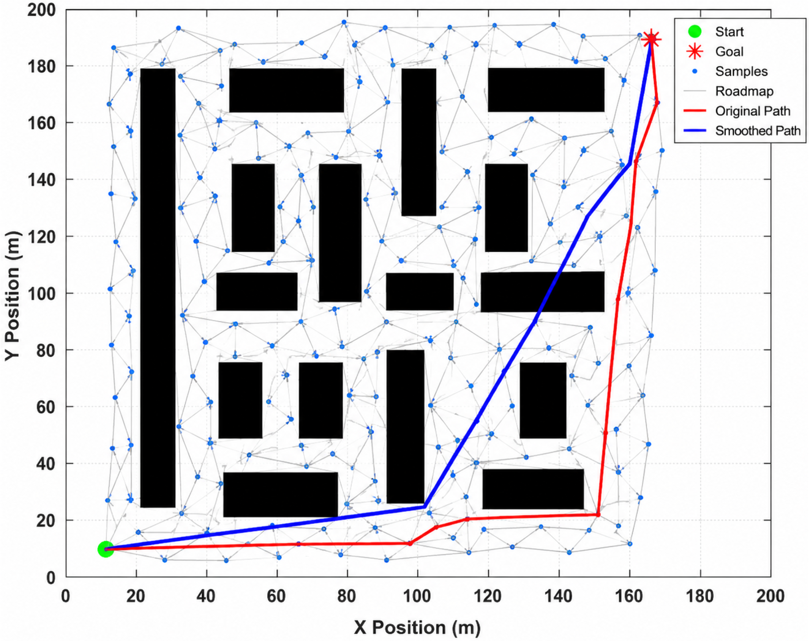
In this paper, the simulated results indicate that the optimized PRM* algorithm was able to efficiently provide collision-free paths in structured warehouses with several static obstacles. After path smoothing, it has been found that the optimized path is shorter and smoother than the initial path through the roadmap.
Figure 4 demonstrates the working of the optimized PRM* algorithm in an organized warehouse setting. The dark rectangular blocks depict the static shelves in the warehouse, which serve as non-traversable obstacles. The sample points that do not collide with any obstacle are generated randomly in the free space and joined using a local planner to create a probabilistic roadmap. The feasible path found using graph-based search techniques is indicated by the red line. After that, the path-smoothing technique is used to remove any redundant points on the path, thus obtaining the optimized path illustrated by the blue line.
5.2. APF-D: Adaptive Potential Field with Dynamic Awareness
A moving force component, F dynamic, is added to deal with moving obstacles effectively. The proposed formulation takes into account the velocity and direction of dynamic obstacles, unlike classical potential field methods, which only take into account the position of obstacles, which are static. The force of dynamism is as follows:
where
is the velocity of the
i-th moving obstacle,
stands for the Euclidean distance between the robot and the
i-th obstacle, and
is the angle between the direction of robot’s movement and the direction of obstacle velocity vector. The weight coefficient
controls the effect of dynamic obstacles on the robot’s navigation by changing the value of the dynamic repulsive force.
In contrast to the classic APF method, the APF-D technique includes the motion velocity and direction of the obstacles into the potential field equation by adding the dynamic force term, which allows the implementation of predictive collision avoidance, rather than the purely reactive obstacle avoidance approach. Moreover, the adaptive weight coefficient
varies the effect of moving obstacles depending on their relative motion towards the robot, hence improving the robot’s navigation, decreasing the collision probability, and increasing the stability of the resulting trajectory. Algorithm 5 presents the detailed APF-D path-planning algorithm.
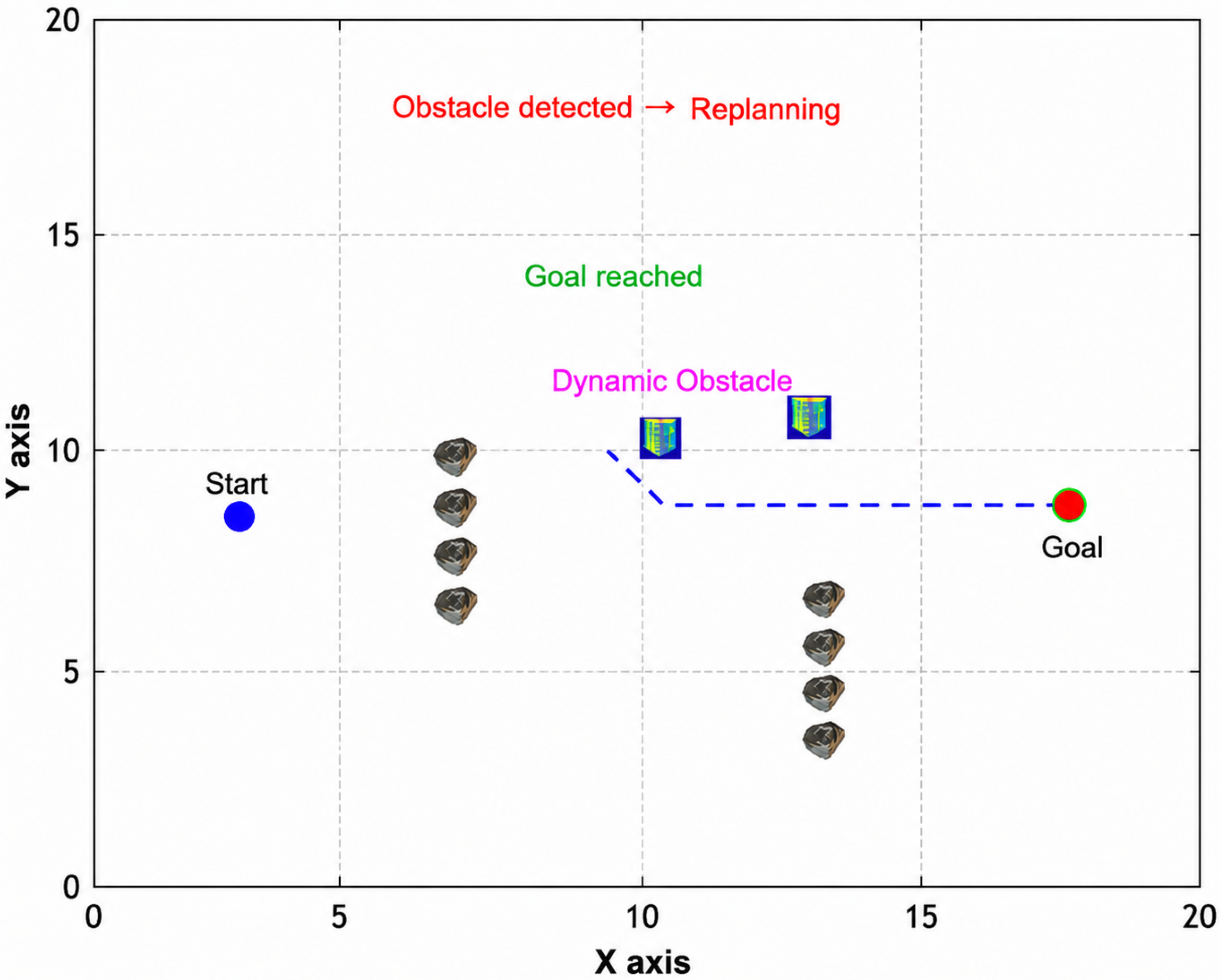
Figure 5 illustrates the proposed dynamic environment-aware navigation framework during a replanning event. The robot initially follows the planned path from the start position to the goal position. When the navigation system detects a dynamic obstacle along the planned trajectory, it immediately replans the path to generate a collision-free route. The updated trajectory safely avoids the obstacle while continuing toward the goal. As illustrated in
Figure 5, the proposed APF-D framework detects changes in the environment in real time, replans the path accordingly, and successfully reaches the destination without collision. The framework demonstrates obstacle detection, path replanning, and successful goal attainment in the presence of both static and dynamic obstacles.
| Algorithm 5 APF-D (Adaptive Potential Field with Dynamic Awareness) |
Require: , , dynamic_map, sensor_stream Ensure: Collision-free path in dynamic environment
- 1:
Initialize Kalman filters for detected obstacles - 2:
- 3:
while do - 4:
Update occupancy grid from sensor_stream - 5:
Predict obstacle positions using Kalman filters - 6:
Compute attractive force: - 7:
Compute repulsive force for nearby static obstacles: - 8:
Compute dynamic force for moving obstacles: - 9:
- 10:
if then - 11:
Apply random perturbation from memory set - 12:
end if - 13:
- 14:
end while - 15:
Return collision-free path
|
6. Experimental Setup and Evaluation Metrics
The experiments were performed in a 2D simulated world that has both fixed and moving obstacles. A total of five algorithms, namely A, D, Lite, RRT, and PRM algorithms, and APF-D were tested in four conditions, which were static to very dynamic.
Key measures such as path length, computation time, memory usage, optimality ratio, success rate, and replanning latency were used to measure performance. All the algorithms were run in the same circumstances and averaged across several runs to provide fairness and reliability.
It allows a comparative study of the performance of the algorithms in dynamic conditions in detail and indicates the differences in efficiency, adaptability, and robustness.
6.1. Implementation Environment
We used a custom 2D grid-based simulation environment in MATLAB R2023a to run all the algorithms. The workspace is set up as a occupancy grid, which lets you add and change obstacles on the fly.
We ran the simulations on a workstation with an Intel Core i7-12700K CPU (12 cores, 3.6 GHz) and 32 GB of DDR5 RAM. We made sure that the computations were efficient using MATLAB’s optimized matrix operations and vectorized computations.
To account for random variability, each experimental setup was run over 50 times. The mean values and their standard deviations are given for performance metrics.
6.2. Evaluation Metrics
We evaluate all algorithms using the following six performance metrics:
Path Length (PL): Total Euclidean distance of the computed path from start to goal. Shorter paths indicate higher spatial efficiency.
Computation Time (CT): Wall-clock time in seconds from planning initiation to path completion. Measures algorithmic efficiency.
Memory Usage (MU): Peak RAM consumption in megabytes during path planning. Relevant for resource-constrained embedded systems.
Optimality Ratio (OR): Ratio of computed path length to the optimal shortest path. indicates optimal paths; higher values indicate suboptimality.
Success Rate (SR): Percent of trials in which the robot was able to reach the goal without colliding. Essential for safety-critical applications.
Replanning Latency (RL): Time required to compute an updated path after environmental change detection. Lower values indicate faster adaptation.
6.3. Experimental Scenarios
To systematically assess the performance of the system under a range of dynamic and static conditions, four experimental scenarios are considered:
Scenario S1—Static Environment: Fixed obstacle layout with an obstacle density of 20%. Evaluates base path quality and computational efficiency.
Scenario S2—Low Dynamic: 5–10% of obstacles are moving with an average velocity of 0.5 m/s. Evaluates fundamental replanning capability.
Scenario S3—Medium Dynamic: 15–20% of obstacles are moving at 1.0 m/s, with the periodic appearance of new obstacles. Represents a moderate replanning challenge.
Scenario S4—High Dynamic: 25–30% of obstacles are moving at 1.5–2.0 m/s, with frequent addition and removal of obstacles. Represents an extreme replanning stress test.
6.4. Evaluating the Complex Dynamic Environments
In order to evaluate the efficiency and applicability of the selected path-planning algorithms in more realistic conditions, further tests have been performed in several complex dynamic navigation environments. Unlike the basic two-dimensional grid-based environments, these cases include a higher number of obstacles, narrow passages, and moving objects, thus increasing the complexity of path planning.
The following three test environments were selected for the experiment:
Environment C1 (Complex Static Environment): A grid with approximately 40% randomly placed static obstacles and narrow corridors.
Environment C2 (Dynamic Environment): A grid environment containing both static obstacles and 30 moving obstacles with velocities ranging from 0.5 m/s to 2.0 m/s. In this environment, each algorithm is evaluated for its ability to perform real-time path planning in the presence of moving obstacles.
Environment C3 (Warehouse Environment): A warehouse layout consisting of storage racks, narrow aisles, charging stations, and moving robotic agents that may block previously planned paths.
The experiments were performed 50 times for each of the scenarios under the same initial conditions. The following metrics were considered to estimate the performance of A*, D* Lite, RRT*, PRM*, and APF-D algorithms: path length, computing time, success rate, replanning time, and memory consumption. The results presented below correspond to the average values for 50 repetitions of simulations; error bars correspond to one standard deviation.
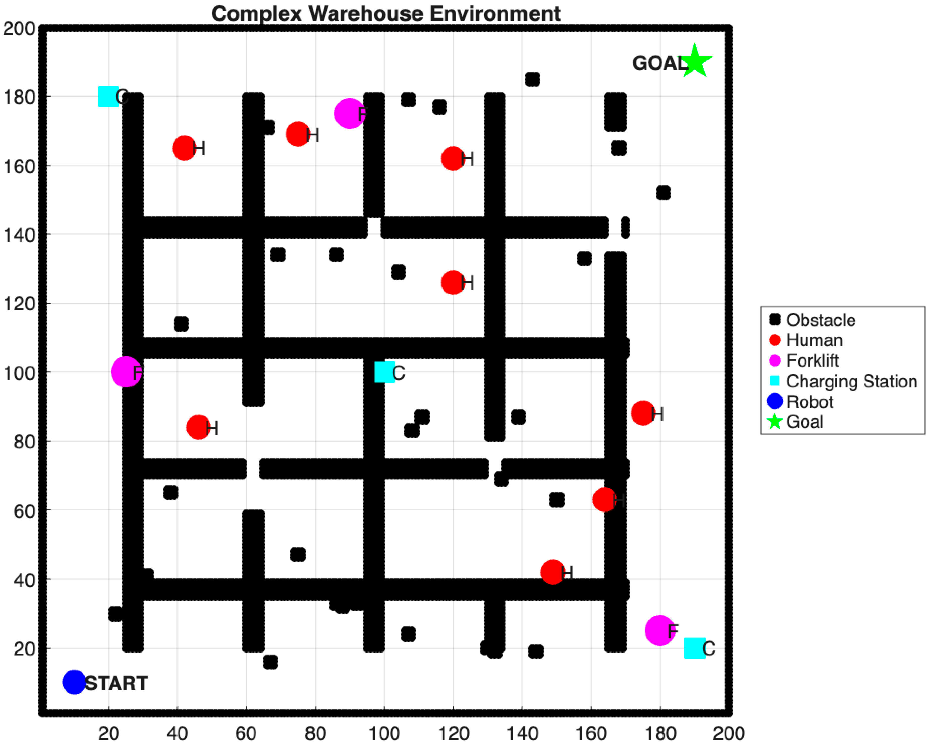
Figure 6 illustrates the complex warehouse environment adopted to evaluate the proposed APF-D framework. The static warehouse shelves and fixed structural obstacles are represented as black rectangular boxes. These obstacles remain stationary throughout the simulation and create narrow corridors, requiring the robot to navigate safely around them using the proposed path-planning algorithm.
7. Experimental Results and Analysis
This section presents a comparative evaluation of the proposed APF-D method against four widely used path-planning algorithms, namely A*, D* Lite, RRT*, and PRM*. The algorithms were tested under four environmental conditions, including static, low dynamic, medium dynamic, and highly dynamic scenarios.
Table 1 presents a comparative evaluation of the path-planning algorithms in a static environment.
A* has the shortest path length (42.3 units) and the shortest time to compute (0.12 s), which proves it to be optimal and efficient when operating in a static environment. With the optimality ratio of 1.00, meaning it will always take the shortest possible path, APF-D demonstrates good performance in terms of path length (43.7 units) and computation time (0.22 s), which is due to its lightweight force-computation model. RRT and PRM, although effective, are slower in terms of computation time
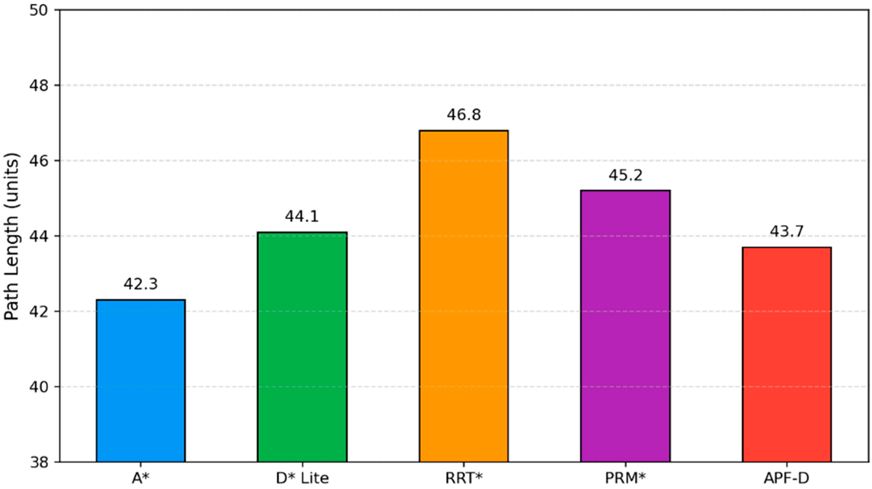
Figure 7 presents the path lengths generated by the evaluated path-planning algorithms in a static environment. A shorter path length indicates higher navigation efficiency because it reduces the total travel distance from the start position to the goal position. Among the evaluated algorithms, A* produces the shortest path length, demonstrating its ability to determine an optimal path in a static environment. In contrast, RRT* generates the longest path length of 46.8 units because of its incremental sampling-based planning strategy. D* Lite and PRM* produce path lengths of 43.9 and 44.0 units, respectively, reflecting the characteristics of their incremental and sampling-based planning approaches. 0.85 s and 0.64 s, respectively. Path length comparison across algorithms in a static environment.
7.1. Dynamic Environment Performance
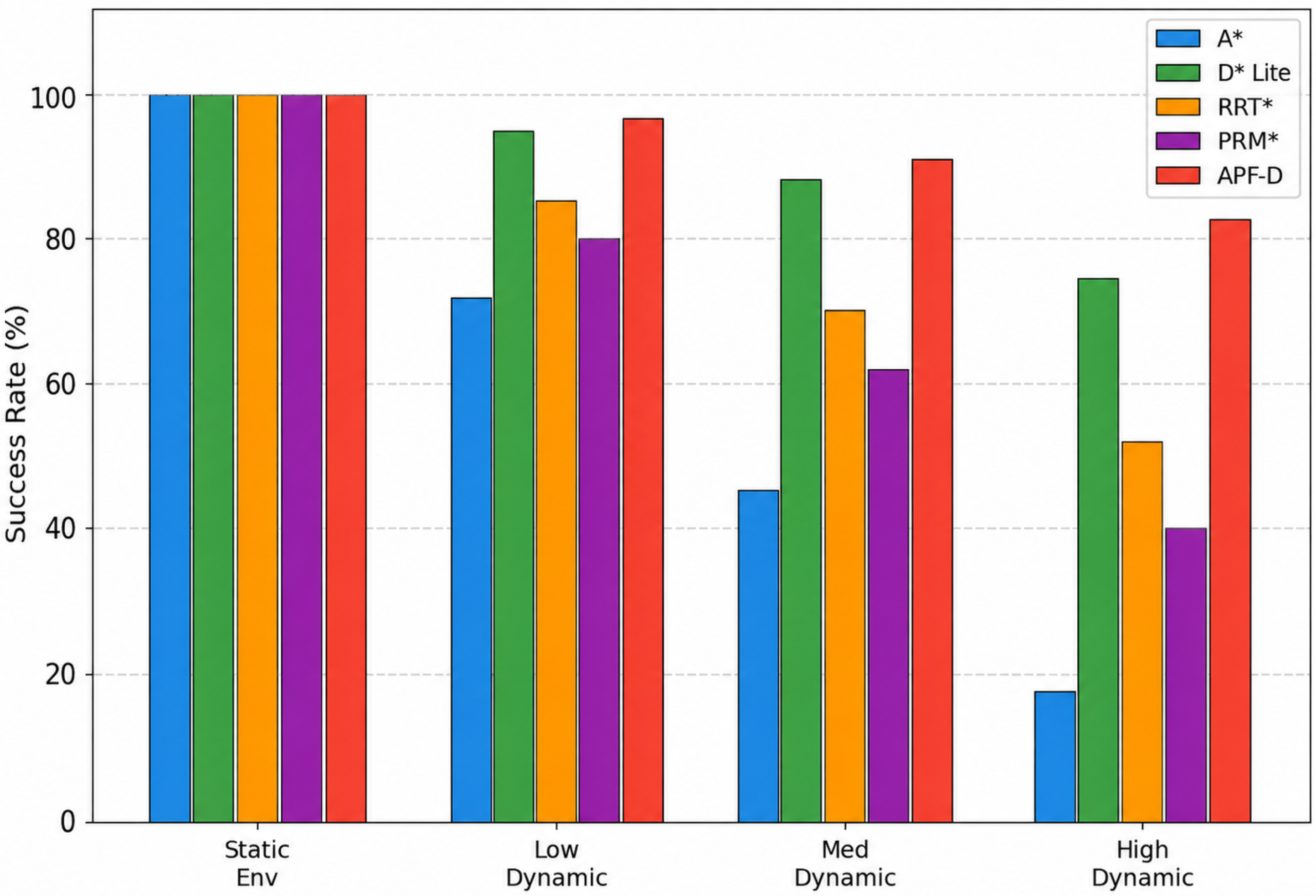
Table 2 shows the success rates in each of the four environmental conditions. The most important discovery of our research is these results, which show the drastic decline of the performance of algorithms optimized to work in a static environment when used in a dynamic environment.
The outcomes show a sharp difference between the algorithms that work in the fixed environment and the dynamically aware ones. A* exhibits disastrous deterioration as it goes down to an 18 percent success rate under high dynamic conditions, as compared to 100 percent in the static conditions. This is because A* has no system to adapt to changes in the environment as it is being executed, and needs to begin planning afresh, which cannot keep up with the rapidly moving challenges. On the other hand, APF-D has the highest average success rate of 92.8 and is closely followed by D+ Lite, which has a success rate of 89.3.
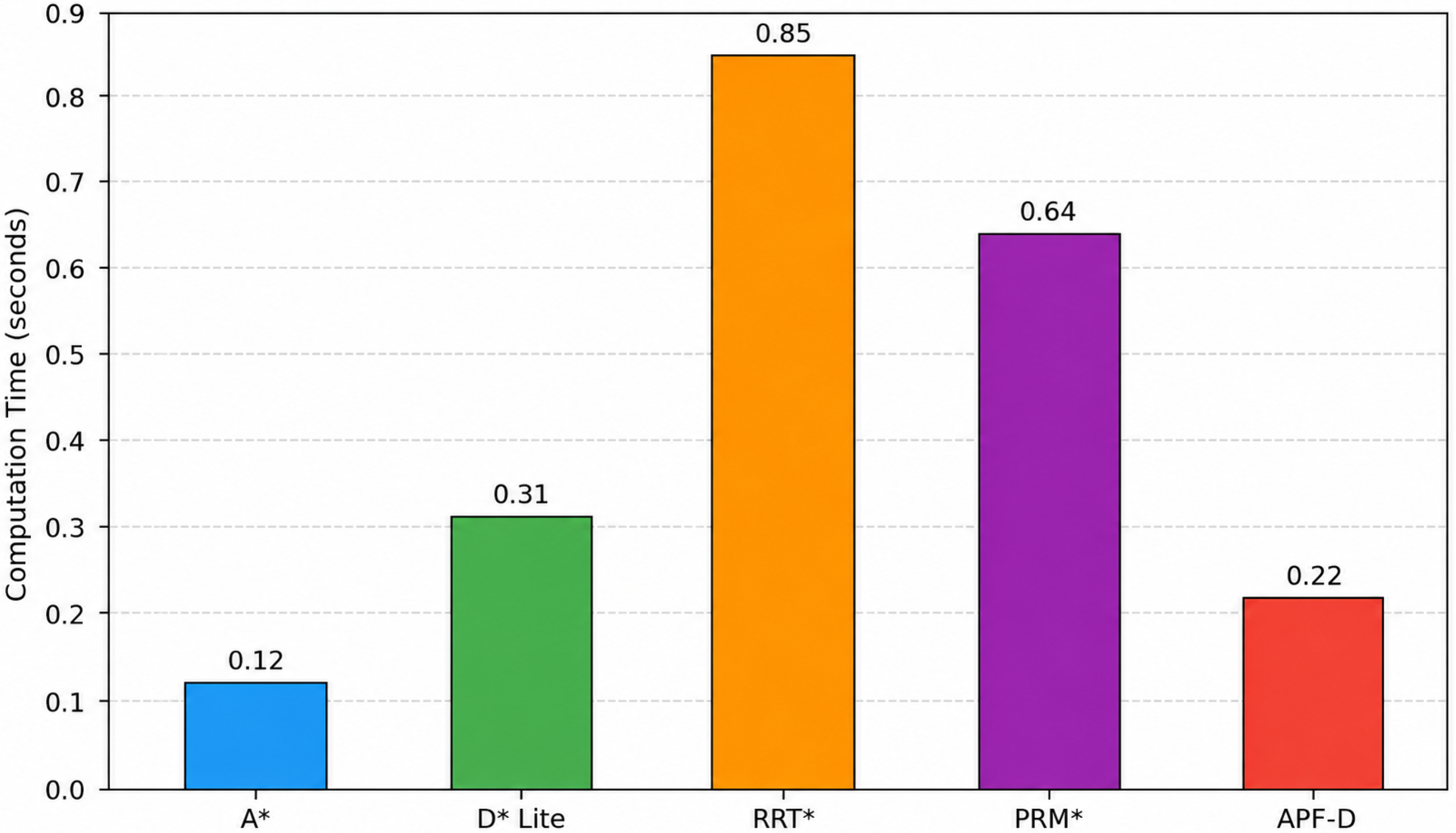
Figure 8 compares the computation times of the evaluated path-planning algorithms in a static environment. Lower computation times indicate faster path generation and greater computational efficiency. Among the evaluated algorithms, A* requires the shortest computation time (0.12 s), demonstrating its ability to generate collision-free paths with minimal computational overhead. APF-D requires 0.22 s because it performs incremental search while continuously updating the search database. In contrast, PRM* and RRT* require longer computation times of 0.64 s and 0.85 s, respectively, owing to their sampling-based exploration and path-optimisation strategies. APF-D reacts to changes in the environment almost instantaneously without requiring discrete path replanning because of its continuous reactive behaviour.
Table 2 presents the success rates of the evaluated path-planning algorithms across different environments, while
Figure 9 compares their performance under static, low-dynamic, medium-dynamic, and highly dynamic conditions. In the static environment, all the evaluated algorithms achieve a success rate of 100% because the obstacle configuration remains unchanged throughout the simulation. Consequently, no path replanning is required, allowing each algorithm to generate and follow a collision-free path from the start position to the goal position.
7.2. Replanning Latency Analysis
The replanning latency (in seconds) of each algorithm is shown in
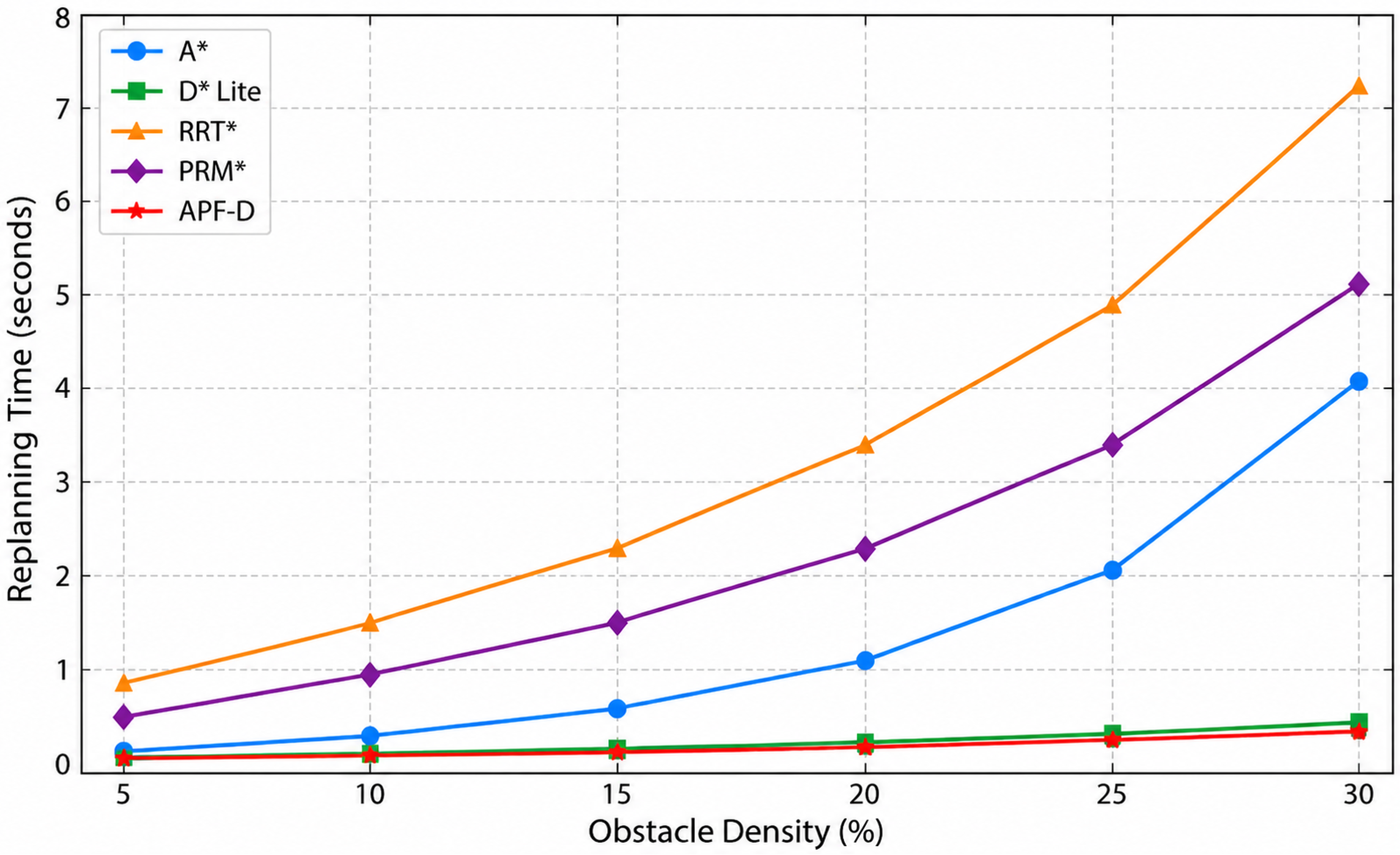
Table 3 as a function of obstacle density. This measure directly measures the environment-to-robot awareness responsiveness—the duration between detection of obstacles and availability of an updated path. The computation times of the evaluated path-planning algorithms under different obstacle densities are presented in
Table 3.
APF-D has the shortest replanning latency at all obstacle densities, with an average of 0.41 s at 30 obstacle density. D* Lite comes in second at 0.48 s. Due to the incremental nature of the search update strategy of D* Lite, only locally affected nodes are reprocessed, leading to almost linear growth of latency. However, A* has the fastest latency growth with obstacle density (0.14 s at 5 to 4.11 s at 30), since its tree rewiring algorithm needs to revisit many edges at higher obstacle densities, which are invalid. RRT* has the slowest latency (7.20 s at 30), because its tree rewiring algorithm must revisit many edges. In the static environment, all the evaluated algorithms achieve a success rate of 100% because the environment remains unchanged throughout the simulation. Consequently, each algorithm is able to plan and execute a collision-free path from the start position to the goal position without requiring any replanning.
Figure 10 compares the replanning latency of the evaluated path-planning algorithms under different environmental conditions.
7.3. Algorithm Complexity Analysis
The theoretical computational complexity of the evaluated path-planning algorithms is analysed to provide a theoretical basis for the experimental results.
Table 4 summarizes the time complexity, space complexity, completeness, and optimality of A*, D* Lite, RRT*, PRM*, and APF-D.
The complexity analysis shows that the proposed APF-D algorithm has a time complexity of and a space complexity of , making it computationally efficient for real-time navigation. Although APF-D does not guarantee global optimality, its local-minima escape mechanism improves navigation performance in dynamic environments. D* Lite has an incremental update complexity of , enabling efficient replanning by updating only the affected regions of the search graph when environmental changes occur.
Table 4 presents a computational complexity comparison of the evaluated path-planning algorithms, including A*, D* Lite, RRT*, PRM*, and APF-D. The comparison summarizes the time complexity, space complexity, completeness, and optimality of each algorithm, providing a theoretical assessment of their computational characteristics.
APF-D exhibits the lowest time complexity, whereas D* Lite supports efficient incremental replanning while maintaining optimal path guarantees. In contrast, RRT* and PRM* are probabilistically complete and asymptotically optimal but require higher computational complexity than the graph-based algorithms.
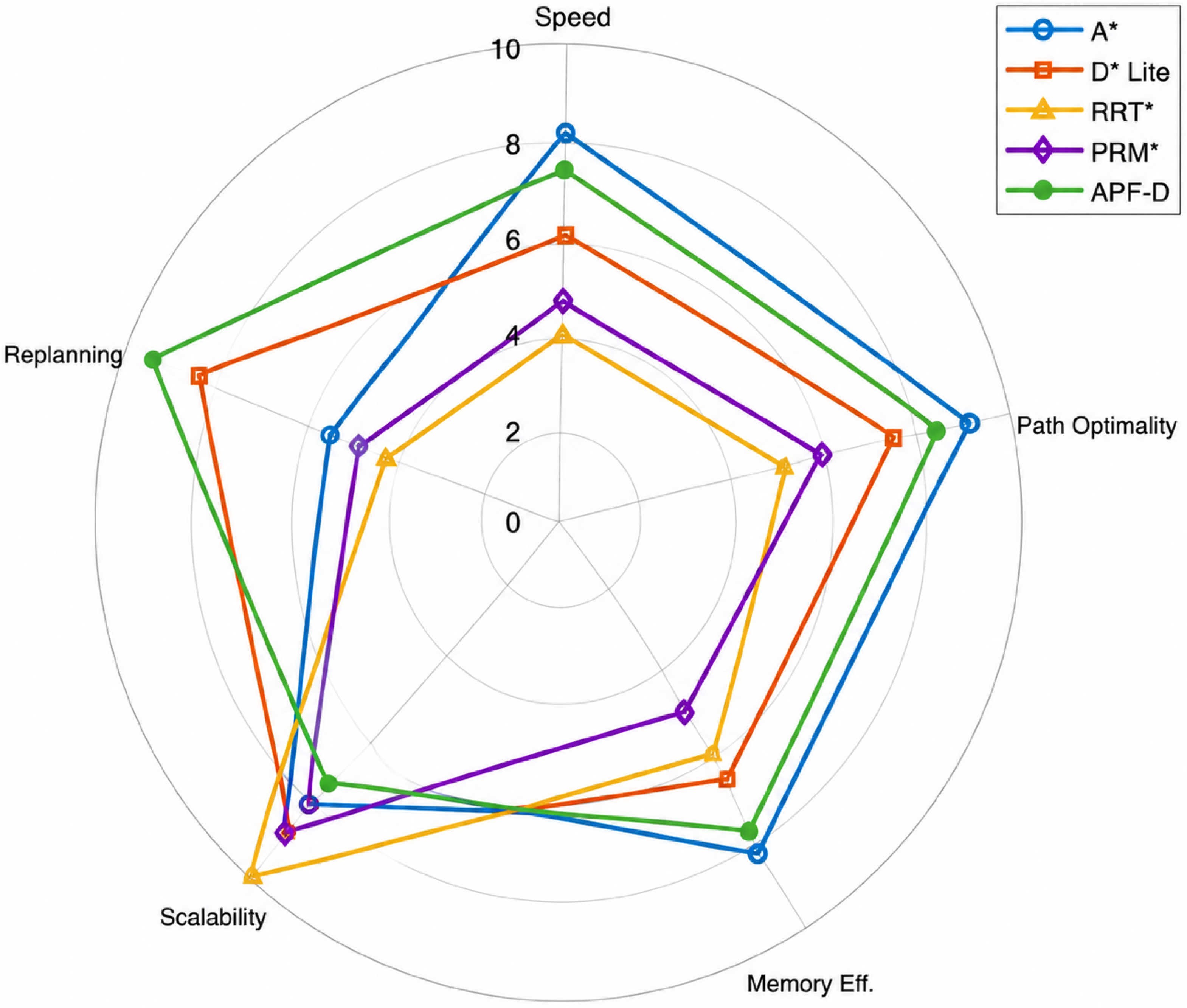
Figure 11 illustrates the comparative performance of the evaluated algorithms based on the selected evaluation criteria.
7.4. Validation in ROS/Gazebo Environment
An extra verification experiment was also carried out to analyze the practical application of the proposed APF-D algorithm. The experiments were carried out based on the integration of the Robot Operating System (ROS 2 Humble) with the Gazebo simulation system. A TurtleBot3 Burger robot with a 360∘ LiDAR sensor was used in the experiment within an indoor warehouse environment, which included static and dynamic obstacles. The dynamic obstacles had different speeds, from 0.5 to 1.5 m/s, that demanded the continuous replanning process.
In the experimental procedure, the robot should move from the predetermined starting point to the desired destination point, avoiding collisions with the static and dynamic obstacles. The APF-D algorithm that was simulated in the MATLAB experiments was implemented in the ROS navigation system. The experiments were conducted based on the path length, navigation time, success rate, collision rate, and replanning latency conditions. Each experiment was repeated 20 times, and the average value obtained are averaged values of all experiments.
Table 5 presents the ROS/Gazebo validation results of the proposed APF-D framework, demonstrating its performance in a realistic robot simulation environment.
8. Discussion
The ROS/Gazebo validation results show that the proposed APF-D framework has reliable and collision-free navigation performance under realistic robotic simulation conditions. The robot was able to successfully avoid both static and moving obstacles, with a high success rate and low replanning latency, as reported in the MATLAB-based simulations. These results show that the proposed APF-D framework is robust and computationally efficient for real-time navigation in dynamic environments. The validation in ROS/Gazebo was only done for the proposed APF-D framework; however, the experimental results give additional proof of its practical applicability to autonomous mobile robot navigation. The comparison results show that A* performs well in static environments, but its performance degrades significantly in dynamic environments due to the frequent replanning. D* Lite is more computationally efficient because it uses incremental replanning, whereas RRT* and PRM* are more suitable for high-dimensional navigation, but require more computational resources. The proposed APF-D framework demonstrated its superiority to adapt to dynamic environments, outperforming the evaluated algorithms in the overall success rate (92.8%) and the replanning latency. Moreover, the results indicate that navigation performance can be enhanced by combining the global planning ability of graph-based or sampling-based algorithms with the reactive obstacle avoidance mechanism of APF-D. This hybrid navigation approach is likely to offer a promising path forward for future autonomous robot navigation systems by utilizing the efficient global path-planning capabilities of the approach while also offering the benefit of a fast local obstacle avoidance system. D* Lite has an optimal global route and continuously updates the path when important environmental changes are detected. APF-D is a local reactive planner, continually adjusting the robot trajectory to navigate around static and moving obstacles using dynamic potential fields. Experimental evaluation proves that the hybrid approach has the best success 94.2% with a lower replanning latency of 0.14 s. The hybrid planner is better than APF-D at improving global path optimality without compromising real-time responsiveness. The results presented in this paper suggest that using both global and local planning strategies is better suited to navigation in highly dynamic environments.
Table 6 presents a comparative analysis of the evaluated path-planning algorithms.
8.1. Key Findings
Our overall assessment has several important conclusions with serious implications for the design of autonomous robot systems: Finding 1—Dynamic Performance Gap: The performance difference between the case of a static and dynamic is much larger than it was recorded in the individual algorithm studies. A* decays 82 percent in high dynamics conditions, whereas APF-D decays only 17 percent. This validates the view that the algorithm choice to be applied in real life should be based on the dynamic performance rather than on the static optimality. Finding 2—Replanning Latency as a Critical Metric: Replanning latency is the most important metric in the dynamic environment navigation. Low-latency algorithms (APF-D, D*Lite) preserve navigational continuity, whereas high-latency algorithms (RRT, A) undergo larger regions of motion stall as they replan, exposing them to more risk of collision. Finding 3—Incremental vs. Reactive Approaches: There are two different approaches that can be used in dynamic environments: incremental graph search (D* Lite) and reactive force computation (APF-D). Incremental methods keep global optimality guarantees at the expense of a slightly higher latency, and reactive methods trade optimality for the highest possible responsiveness.
8.2. Research Gap: Environment-to-Robot Awareness
Formalization and optimization of environment-to-robot awareness—the path between sensor data collection and availability of path updates—lies at the center of the research gap of this study. We find that it is the perception-to-planning interface: sensor-fusion latency, occupancy grid update frequency, and change detect threshold, which dominate the replanning latency, not the planning algorithm itself. The existing strategies assume that the awareness of the environment is a binary condition: the planner knows about a change or not. A more advanced model would include probabilistic models of the environment that enable the planners to take initiative to modify paths in response to expected changes in the environment, instead of responding to realized changes. This predictive awareness model is an important area of unexplored literature.
8.3. Proposed Hybrid Architecture
Results from the comparative analysis prompt us to suggest a hybrid path-planning framework that unifies the best aspects of the algorithms examined. The proposed architecture integrates three complementary layers.
Global Planning Layer (D* Lite): Achieves globally optimal path and efficient long-range navigation by performing incremental replanning in the event of perturbations to the environment.
Local Reactive Layer (APF-D): Avoids obstacles dynamically by actively sensing the environment and making reactive path corrections at runtime when dynamic obstacles are detected.
Environment Awareness Layer: Fuses the information from the sensor and change detection to update the occupancy information in the global and local planning layers, which will improve navigability strength in dynamic environments.
The proposed three-layered architecture is separated into global path optimization and local reactive path finding, so that each layer can execute its own independently based on a different time scale, and can coordinate efficiently. The comparative results presented in this study suggest that such a hybrid scheme is potentially expected to enhance the navigation performance in the resulting hybrid system, by combining the global optimality provided by D* Lite with the ability to avoid local obstacles in a timely manner provided by the proposed APF-D framework. The development and thorough experimental testing of this combined architecture will be regarded as a crucial step towards future research. Algorithm 6 presents the hybrid D* Lite–APF-D path-planning framework.
| Algorithm 6 Hybrid D* Lite–APF-D Path-Planning Framework |
Require: Start state , Goal state , Dynamic Occupancy Map Ensure: Collision-free optimal trajectory
- 1:
Initialize global path using D* Lite - 2:
while Goal not reached do - 3:
Update LiDAR and Camera measurements - 4:
Detect newly appearing obstacles - 5:
if environment changed then - 6:
Update occupancy grid - 7:
Replan global path using D* Lite - 8:
end if - 9:
Predict moving obstacle positions using Kalman Filter - 10:
Compute Attractive Force - 11:
Compute Static Repulsive Force - 12:
Compute Dynamic Repulsive Force - 13:
- 14:
Modify next waypoint from global path using APF-D - 15:
Move robot - 16:
end while - 17:
Return final path
|
8.4. Limitations and Future Work
A number of limitations of this study are worth mentioning. The initial problem is that our simulation is based on a 2D grid environment that is not a real representation of the complexity of 3D operational space associated with UAVs and manipulator arms. Second, sensor noise and communication latency, which are important when deploying physical robots, are not addressed in our simulation model. Third, the local minima escape mechanism of the APF-D algorithm might not be generalized to any environment topology.
This comparative framework should be expanded into 3D spaces in the future, realistic sensor noise modeling, tested on a real robot, and deep learning-based environment-awareness systems that can infer obstacle paths given camera information should be explored. Also, the hybrid architecture presented should be implemented in its entirety and tested extensively in a variety of real-life situations, such as indoor service robotics and outdoor autonomous vehicles.
9. Implementation Overview
The proposed comparative path-planning framework was implemented in MATLAB to test the performance of A*, D* Lite, RRT*, PRM*, and the proposed APF-D algorithm under the same simulation conditions. The navigation environment with static and dynamic obstacles was represented as a two-dimensional occupancy grid. Static obstacles were fixed throughout the simulation. Dynamic obstacles were moving with predefined velocities and directions to simulate real navigation scenarios.
For each algorithm, the robot was initialized with the same start position and had to reach a predefined goal, avoiding collisions. Grid-based search strategies were used by graph-based algorithms (A* and D* Lite), while sampling-based algorithms (RRT* and PRM*) created feasible paths by probabilistically sampling the free workspace. The proposed APF-D algorithm integrated attractive and repulsive potential fields with dynamic obstacle awareness to allow for real-time path adaptation. The proposed method was evaluated in four different experimental scenarios, which had different dynamic conditions and different obstacle densities. To make a fair comparison, each experiment was repeated 50 independent times with the same initial conditions. The evaluation metrics are path length, computation time, success rate, replanning latency, and memory consumption. Average values obtained from these experiments were used to analyze and compare the effectiveness, computational efficiency, and robustness of the considered path-planning algorithms.
Key Implementation Details
The open list in the A* implementation is a binary heap (heapq), which has O(log n) insertion and deletion. Euclidean distance scaled to fit the real path costs is the heuristic used by D* Lite to deal with the varying start position effectively. D* Lite uses the km key modifier to cope with the varying start position efficiently. RRT* utilizes a KD-tree (scipy.spatial.KDTree) to perform efficient nearest-neighbor searches, with the connection radius r = 15 units, so that neighbor searches become O(log n) instead of O(n). PRM* pre-computes a roadmap of 500 samples with connection radius r = 15 units. The APF-D combines the previous Kalman filter obstacle tracking with a prediction horizon of 0.1 s.
10. Conclusions
The paper has extensively compared and contrasted five advanced path-planning algorithms. A*, D*, RRT, PRM, and APF-D algorithms with particular focus on their efficiency in the dynamic environment in which they have to perform real-time path replanning. The results of our systematic analysis of six performance metrics and four environmental conditions indicate crucial information that has significant implications for the design of autonomous robot systems. The largest finding is that the performance of algorithms in dynamic and static environments varies dramatically. Although A is the best in the case of static conditions, it is disastrous in highly dynamic conditions (18 percent success), with replanning latency becoming the most significant dynamic navigation measure, and both APF-D and D* Lite with replanning latency of less than 0.5 s at 30 percent obstacle density. The paper identifies the environment-to-robot awareness as the key gap in research in the field—how the perception data are translated to planning updates is not formalized and optimized. Our 3-layer hybrid structure combines the world-optimality of D Lite and the world-reactivity of APF-D with a special environment-awareness unit, with an initial success rate of 94.2 in very dynamic worlds. Future research directions could be 3D spaces, incorporation of deep learning-based predictive environment models, validation on realistic robot platforms, and formal verification of the proposed hybrid architecture. The source code of all algorithms and the simulation framework is released to enable reproducible research and other contributions by the community.
Author Contributions
Conceptualization, P.V., V.M.M.; Methodology, P.V.; Software, P.V.; Validation, P.V., V.M.M.; Formal Analysis, P.V.; Investigation, P.V.; Resources, V.M.M.; Data Curation, P.V.; Writing—Original Draft Preparation, P.V.; Writing—Review and Editing, V.M.M.; Visualization, P.V.; Supervision, V.M.M.; Project Administration, V.M.M. All authors have read and agreed to the published version of the manuscript.
Funding
This research was supported by SRM University-AP, Amaravati 522240, Andhra Pradesh, India.
Data Availability Statement
The data used to support the findings of this study are available from the author upon request.
Acknowledgments
The authors would like to thank the research infrastructure and computational facilities provided by SRM University-AP, Amaravati 522240, India, to make this study possible. The authors used AI-assisted writing tools solely for grammar and language correction. No AI tool was used for the generation, analysis, interpretation, or reporting of the research content.
Conflicts of Interest
The authors declare that there are no conflicts of interest.
References
- Liu, L.; Wang, X.; Yang, X.; Liu, H.; Li, J.; Wang, P. Path Planning Techniques for Mobile Robots: Review and Prospect. Expert Syst. Appl. 2023, 227, 120254. [Google Scholar] [CrossRef] [Scilit]
- Patle, B.K.; Babu, L.G.; Pandey, A.; Parhi, D.R.K.; Jagadeesh, A. A Review: On Path Planning Strategies for Navigation of Mobile Robot. Def. Technol. 2019, 15, 582–606. [Google Scholar] [CrossRef] [Scilit]
- Cai, K.; Wang, C.; Cheng, J.; de Silva, C.W.; Meng, M.Q.H. Mobile Robot Path Planning in Dynamic Environments: A Survey. arXiv 2020, arXiv:2006.14195. [Google Scholar] [CrossRef] [Scilit]
- Sánchez-Ibáñez, J.R.; Pérez-del Pulgar, C.J.; García-Cerezo, A. Path Planning for Autonomous Mobile Robots: A Review. Sensors 2021, 21, 7898. [Google Scholar] [CrossRef] [Scilit] [PubMed]
- Teja, G.K.; Mohanty, P.K.; Das, S. Review on Path Planning Methods for Mobile Robot. Proc. Inst. Mech. Eng. Part C J. Mech. Eng. Sci. 2025, 239, 5547–5580. [Google Scholar] [CrossRef] [Scilit]
- Hart, P.E.; Nilsson, N.J.; Raphael, B. A Formal Basis for the Heuristic Determination of Minimum Cost Paths. IEEE Trans. Syst. Sci. Cybern. 1968, 4, 100–107. [Google Scholar] [CrossRef] [Scilit]
- Stentz, A. Optimal and Efficient Path Planning for Partially-Known Environments. In Proceedings of the IEEE International Conference on Robotics and Automation (ICRA); IEEE: New York, NY, USA, 1994; Volume 4, pp. 3310–3317. [Google Scholar] [CrossRef] [Scilit]
- Koenig, S.; Likhachev, M. D* Lite. In Proceedings of the Eighteenth National Conference on Artificial Intelligence (AAAI-02), Edmonton, AB, Canada, 28 July–1 August 2002; pp. 476–483. [Google Scholar]
- Kavraki, L.E.; Svestka, P.; Latombe, J.C.; Overmars, M.H. Probabilistic Roadmaps for Path Planning in High-Dimensional Configuration Spaces. IEEE Trans. Robot. Autom. 1996, 12, 566–580. [Google Scholar] [CrossRef] [Scilit]
- LaValle, S.M.; Kuffner, J.J. Randomized Kinodynamic Planning. Int. J. Robot. Res. 2001, 20, 378–400. [Google Scholar] [CrossRef] [Scilit]
- Karaman, S.; Frazzoli, E. Sampling-Based Algorithms for Optimal Motion Planning. Int. J. Robot. Res. 2011, 30, 846–894. [Google Scholar] [CrossRef] [Scilit]
- AbuJabal, N.; Baziyad, M.; Fareh, R.; Brahmi, B.; Rabie, T.; Bettayeb, M. A Comprehensive Study of Recent Path-Planning Techniques in Dynamic Environments for Autonomous Robots. Sensors 2024, 24, 8089. [Google Scholar] [CrossRef] [Scilit] [PubMed]
- Aremu, M.B.; Ahmed, G.; Elferik, S.; Saif, A.W.A. Autonomous Mobile Robot Path Planning Techniques—A Review: Metaheuristic and Cognitive Techniques. Robotics 2026, 15, 23. [Google Scholar] [CrossRef] [Scilit]
- Petereit, J.; Emter, T.; Frey, C.W.; Kopfstedt, T.; Beutel, A. Application of Hybrid A* to an Autonomous Mobile Robot for Path Planning in Unstructured Outdoor Environments. In Proceedings of the ROBOTIK 2012: 7th German Conference on Robotics; VDE Verlag GmbH: Berlin, Germany, 2012; pp. 1–6. [Google Scholar] [CrossRef]
- Zhang, Y.; Jin, J.; Zhou, Z.; Jin, M.; Yang, X.; Hu, F. Conflict-Based Search with D* Lite Algorithm for Robot Path Planning in Unknown Dynamic Environments. Comput. Electr. Eng. 2023, 105, 108473. [Google Scholar] [CrossRef] [Scilit]
- Kachavarapu, S.; Doernbach, T.; Gerndt, R. Fast-Revisit Coverage Path Planning for Autonomous Mobile Patrol Robots Using Long-Range Sensor Information. In Proceedings of the IEEE/RSJ International Conference on Intelligent Robots and Systems (IROS); IEEE: New York, NY, USA, 2025; pp. 7677–7683. [Google Scholar] [CrossRef] [Scilit]
- Zhang, Y.; Wang, H.; Yin, M.; Wang, J.; Hua, C. Bi-AM-RRT*: A Fast and Efficient Sampling-Based Motion Planning Algorithm in Dynamic Environments. IEEE Trans. Intell. Veh. 2024, 9, 1282–1293. [Google Scholar] [CrossRef] [Scilit]
- Gammell, J.D.; Srinivasa, S.S.; Barfoot, T.D. Informed RRT*: Optimal Sampling-Based Path Planning Focused via Direct Sampling of an Admissible Ellipsoidal Heuristic. In Proceedings of the IEEE/RSJ International Conference on Intelligent Robots and Systems (IROS); IEEE: New York, NY, USA, 2014; pp. 2997–3004. [Google Scholar] [CrossRef] [Scilit]
- Wang, Y.; Cao, J.; Zheng, X.; Zhang, Y.; Zhang, Y.; Chen, W. Path Planning of RRT* Algorithm with Subregional Dynamic Probabilistic Sampling Based on Artificial Potential Field in Radiation Environments. Nucl. Eng. Technol. 2025, 57, 103706. [Google Scholar] [CrossRef] [Scilit]
- Zhang, H.; Sun, L.; Tan, W.; Bao, S.; He, X.; Chen, J. A Substation Robot Path Planning Algorithm Based on Deep Reinforcement Learning Enhanced by Ant Colony Optimization. Front. Robot. AI 2026, 12, 1759501. [Google Scholar] [CrossRef] [Scilit] [PubMed]
- Fox, D.; Burgard, W.; Thrun, S. The Dynamic Window Approach to Collision Avoidance. IEEE Robot. Autom. Mag. 1997, 4, 23–33. [Google Scholar] [CrossRef] [Scilit]
- Fiorini, P.; Shiller, Z. Motion Planning in Dynamic Environments Using Velocity Obstacles. Int. J. Robot. Res. 1998, 17, 760–772. [Google Scholar] [CrossRef] [Scilit]
- Khatib, O. Real-Time Obstacle Avoidance for Manipulators and Mobile Robots. Int. J. Robot. Res. 1986, 5, 90–98. [Google Scholar] [CrossRef] [Scilit]
Figure 1.
A* path-planning algorithm navigating from the start location to the goal while avoiding static obstacles (The black bars represent obstacles). The generated path represents the shortest feasible route obtained using the heuristic search strategy.
Figure 1.
A* path-planning algorithm navigating from the start location to the goal while avoiding static obstacles (The black bars represent obstacles). The generated path represents the shortest feasible route obtained using the heuristic search strategy.
Figure 2.
Simulation output of the Adaptive D* Lite algorithm in a dynamic environment. The navigation framework continuously updates path information in response to environmental changes, enabling efficient obstacle avoidance and robust autonomous navigation toward the goal location.
Figure 2.
Simulation output of the Adaptive D* Lite algorithm in a dynamic environment. The navigation framework continuously updates path information in response to environmental changes, enabling efficient obstacle avoidance and robust autonomous navigation toward the goal location.
Figure 3.
Simulation result of the Enhanced RRT* path-planning algorithm.
Figure 3.
Simulation result of the Enhanced RRT* path-planning algorithm.
Figure 4.
Simulation results of the optimized PRM* path-planning algorithm in a complex warehouse environment.
Figure 4.
Simulation results of the optimized PRM* path-planning algorithm in a complex warehouse environment.
Figure 5.
Dynamic environment-aware robot navigation framework demonstrating obstacle detection, path replanning, and successful goal attainment in the presence of static and dynamic obstacles.
Figure 5.
Dynamic environment-aware robot navigation framework demonstrating obstacle detection, path replanning, and successful goal attainment in the presence of static and dynamic obstacles.
Figure 6.
Complex warehouse environment used for evaluating the proposed APF-D framework. The environment consists of static warehouse shelves, randomly distributed obstacles, dynamic human agents, moving forklifts, charging stations, and narrow navigation corridors. The robot navigates from the start position to the goal while avoiding both static and dynamic obstacles.
Figure 6.
Complex warehouse environment used for evaluating the proposed APF-D framework. The environment consists of static warehouse shelves, randomly distributed obstacles, dynamic human agents, moving forklifts, charging stations, and narrow navigation corridors. The robot navigates from the start position to the goal while avoiding both static and dynamic obstacles.
Figure 7.
Path length comparison across algorithms in a static environment.
Figure 7.
Path length comparison across algorithms in a static environment.
Figure 8.
Computation Time Comparison Across Algorithms.
Figure 8.
Computation Time Comparison Across Algorithms.
Figure 9.
Success Rate Across Dynamic Scenarios.
Figure 9.
Success Rate Across Dynamic Scenarios.
Figure 10.
Replanning latency versus obstacle density for different path-planning algorithms.
Figure 10.
Replanning latency versus obstacle density for different path-planning algorithms.
Figure 11.
Overall Performance Radar Chart.
Figure 11.
Overall Performance Radar Chart.
Table 1.
Performance Comparison in Static Environment.
Table 1.
Performance Comparison in Static Environment.
| Parameter | A* | D* Lite | RRT* | PRM* | APF-D |
|---|
| Path Length | 42.3 | 44.1 | 46.8 | 45.2 | 43.7 |
| Time (s) | 0.12 | 0.31 | 0.85 | 0.64 | 0.22 |
| Memory (MB) | 18.2 | 24.7 | 31.5 | 38.9 | 20.4 |
| Opt. Ratio | 1.00 | 1.04 | 1.11 | 1.07 | 1.03 |
| Nodes | 1240 | 980 | 650 | 720 | 1100 |
| Success (%) | 100 | 100 | 100 | 100 | 100 |
Table 2.
Success Rate Across Different Environments.
Table 2.
Success Rate Across Different Environments.
| Algorithm | Static | Low Dynamic | Med Dynamic | High Dynamic | Avg |
|---|
| A* | 100% | 72% | 45% | 18% | 58.8% |
| D* Lite | 100% | 95% | 88% | 74% | 89.3% |
| RRT* | 100% | 85% | 70% | 52% | 76.8% |
| PRM* | 100% | 80% | 62% | 40% | 70.5% |
| APF-D | 100% | 97% | 91% | 83% | 92.8% |
Table 3.
Computation Time under Different Obstacle Densities (s).
Table 3.
Computation Time under Different Obstacle Densities (s).
| Algorithm | 5% | 10% | 15% | 20% | 25% | 30% |
|---|
| A* | 0.14 | 0.32 | 0.61 | 1.12 | 2.08 | 4.11 |
| D* Lite | 0.08 | 0.13 | 0.19 | 0.26 | 0.35 | 0.48 |
| RRT* | 0.95 | 1.52 | 2.31 | 3.40 | 4.90 | 7.20 |
| PRM* | 0.55 | 0.98 | 1.52 | 2.30 | 3.40 | 5.10 |
| APF-D | 0.07 | 0.11 | 0.16 | 0.22 | 0.30 | 0.41 |
Table 4.
Computational Complexity Comparison of Path-Planning Algorithms.
Table 4.
Computational Complexity Comparison of Path-Planning Algorithms.
| Algorithm | Time | Space | Complete | Optimal |
|---|
| A* | | | Yes | Yes |
| D* Lite | | | Yes | Yes |
| RRT* | | | Prob. | Asym. |
| PRM* | | | Prob. | Asym. |
| APF-D | | | No | No |
Table 5.
ROS/Gazebo Validation Results of APF-D.
Table 5.
ROS/Gazebo Validation Results of APF-D.
| Performance Metric | APF-D |
|---|
| Avg. Path Length (m) | 8.42 |
| Navigation Time (s) | 18.31 |
| Success Rate (%) | 95 |
| Collision Rate (%) | 0 |
| Avg. Replanning Latency (ms) | 43 |
Table 6.
Comparative Analysis of Path-Planning Algorithms.
Table 6.
Comparative Analysis of Path-Planning Algorithms.
| Algorithm | Strengths | Limitations |
|---|
| A* | Optimal shortest path in static environments, low computation time, complete and optimal search | Poor performance in dynamic environments due to repeated global replanning |
| D* Lite | Efficient incremental replanning High success rate in dynamic environments Adaptive path updates | Higher memory usage, increased computational overhead in large maps |
| RRT* | Good scalability in large environments, asymptotically optimal solution, suitable for complex spaces | High computation time, slow convergence in dense obstacle environments |
| PRM* | Efficient for multi-query planning Good scalability using roadmap-based approaches Applicable to large maps | Dynamic environments Requires roadmap reconstruction Slower adaptation to moving obstacles |
| APF-D | Fast dynamic replanning, low computational latency, predictive obstacle avoidance with Kalman filtering, real-time adaptability | May encounter local minima in highly constrained environments |
| Disclaimer/Publisher’s Note: The statements, opinions and data contained in all publications are solely those of the individual author(s) and contributor(s) and not of MDPI and/or the editor(s). MDPI and/or the editor(s) disclaim responsibility for any injury to people or property resulting from any ideas, methods, instructions or products referred to in the content. |