Mobile Robot Localization and SLAM: A Critical Review of Sensors, Multi-Sensor Fusion, and Neural Representations

Abstract

Accurate and robust localization remains the fundamental bottleneck for truly autonomous robotic systems, despite decades of progress in probabilistic estimation and SLAM. This paper provides a critical and comprehensive review of mobile robot localization across sensing modalities, estimation paradigms, and deployment domains, covering ground, aerial, and underwater platforms. Beyond a descriptive survey, we explicitly analyze the limitations and trade-offs of existing approaches. We introduce an updated taxonomy that spans classical proprioceptive and exteroceptive sensors, emerging technologies such as 4D imaging radar and event cameras, and infrastructure-based positioning systems including GNSS and Ultra-Wideband. We revisit the evolution of localization algorithms, from Bayesian filtering techniques (EKF, UKF, and particle filters) to modern graph-based SLAM frameworks and tightly coupled multi-sensor fusion systems. Particular emphasis is placed on the recent paradigm shift toward learning-based and neural implicit approaches, including NeRF-SLAM and Gaussian Splatting, highlighting both their transformative potential and their current impracticality for real-time deployment. Unlike previous surveys, this work provides a unified cross-domain perspective while critically examining scalability, robustness, computational cost, and real-world deployability. We identify key unresolved challenges, including long-term consistency, operation in degraded environments, and the integration of semantic understanding into localization pipelines. Furthermore, we propose standardizing evaluation metrics with a formal Trajectory Completeness formulation to expose tracking brittleness. Finally, we outline future research directions toward resilient, certifiable, and truly autonomous localization systems, emphasizing the critical transition from passive estimation to Active SLAM in unstructured environments.

1. Introduction

The fundamental question in mobile robotics, “Where am I?”, remains one of the most intensely researched problems in the field despite decades of advancements [1]. Localization is not merely about computing a coordinate; it is about estimating a robot’s full pose (position and orientation) with quantified uncertainty within a well-defined reference frame. As mobile robots transition from controlled factory floors to complex, unstructured, and highly dynamic environments, from dense urban canyons for autonomous cars to GPS-denied indoor spaces for micro-UAVs and the deep ocean for AUVs, the requirements for localization systems have become increasingly stringent [2].

Historically, mobile robot localization evolved from simple dead-reckoning approaches based on wheel encoders [3] to sophisticated probabilistic frameworks. The seminal work of Smith, Self, and Cheeseman on the stochastic map [4] and its extension to the Simultaneous Localization and Mapping (SLAM) problem by Leonard and Durrant-Whyte [5] established the theoretical foundations that continue to underpin modern systems. The subsequent development of particle-filter-based Monte Carlo Localization (MCL) by Dellaert et al. [6] and Fox et al. [7] brought global localization within known maps to practical maturity. Concurrently, the emergence of visual odometry [8] and keyframe-based visual SLAM [9,10] shifted the community’s focus toward camera-based systems.

In recent years, the field has undergone a paradigm shift driven by three converging trends: (1) the maturation of tightly-coupled multi-sensor fusion frameworks that combine vision, LiDAR, IMU, and GNSS into unified optimization backends [11,12]; (2) the integration of deep learning for feature extraction, place recognition, and end-to-end pose estimation [13,14,15]; and (3) the emergence of neural scene representations, namely Neural Radiance Fields (NeRFs) [16] and 3D Gaussian Splatting (3DGS) [17], that are reshaping how maps are constructed and maintained within SLAM pipelines [18].

Despite this extraordinary progress, fundamental limitations persist: current SLAM systems still struggle with long-term autonomy and dynamic environments; learning-based approaches remain constrained by their dependence on large-scale training data and limited generalization to unseen conditions; and, to the best of our knowledge, a fully unified localization framework that is simultaneously accurate, robust, real-time, and deployable across domains has not yet been achieved. This review confronts these limitations directly, providing a critical and unified cross-domain perspective on the current state of the art. Section 2 describes the literature selection methodology. Section 3 compares this work with existing surveys. Section 4 presents a comprehensive taxonomy of sensor modalities. Section 5 surveys the benchmark datasets and evaluation metrics used throughout this review. Section 6 reviews classical probabilistic state estimation. Section 7 surveys modern SLAM frameworks across visual, LiDAR, radar, and multi-modal paradigms. Section 8 covers end-to-end neural mapping and SLAM pipelines, including NeRF and 3DGS approaches. Section 9 examines deep learning modules for relocalization and feature extraction. Section 10 discusses multi-robot collaborative localization. Section 11 examines deployment domains and real-world challenges across all platform types, including a dedicated analysis of on-board compute platforms (Section 11.7) that quantifies hardware–algorithm compatibility boundaries, consolidating domain-specific constraints with the gap between laboratory evaluation and production deployment. Section 12 discusses fundamental limitations of current approaches. Section 13 identifies open challenges and future research directions, and Section 14 draws conclusions.

1.1. Contributions of This Survey

This paper provides an updated and cross-domain review of localization and mapping for mobile robotics. In contrast to previous surveys that focus on individual paradigms or specific robot platforms, this work aims to unify recent developments across sensing, estimation, and learning-based approaches.

The main contributions of this survey are as follows:

• Unified cross-domain perspective. We review localization and SLAM across ground, aerial, marine, and legged robots, highlighting shared challenges and domain-specific constraints.
• Integration of classical and learning-based pipelines. We provide a structured comparison between probabilistic estimation, geometric SLAM, and emerging neural and foundation-model-based approaches.
• Comprehensive sensor taxonomy. We present an updated overview of sensing modalities, including event cameras, 4D radar, UWB, and multi-modal fusion strategies.
• Analysis of neural SLAM and implicit mapping. We review recent advances in neural radiance fields, differentiable rendering, and learned localization pipelines.
• Benchmark and dataset consolidation. We summarize widely used datasets and evaluation protocols across multiple robotic domains.
• Critical discussion and open research challenges. We identify limitations of current systems and outline future research directions toward robust, scalable, and certifiable localization.

1.2. Operational Definitions

To ensure consistent interpretation throughout this review, the following operational definitions are adopted:

• Real-time: A localization system is considered real-time if it produces a pose estimate at a rate sufficient to close the control loop of the robot without inducing instability. For most ground and aerial platforms, this implies a minimum update rate of 10 Hz; for high-speed UAVs it implies ≥ 50 Hz. Systems requiring offline post-processing, batch optimization, or GPU inference exceeding one frame latency are not classified as real-time.
• Robustness: The ability of a system to maintain bounded localization error across a defined range of environmental perturbations (illumination changes, dynamic objects, adverse weather, and sensor degradation) without manual intervention or re-initialization. Robustness is environment- and sensor-specific; a system may be robust indoors but fragile outdoors.
• Generalization: The capacity of a learned model to produce reliable outputs in environments, sensor configurations, or conditions not represented in the training distribution. Generalization is evaluated by testing on held-out scenes or cross-dataset protocols.
• Deployment-ready: A system is deployment-ready if it has been demonstrated on a physical robot platform under representative operational conditions (not only in controlled laboratory settings or on offline datasets), with reported performance metrics including failure rates.
• Long-term autonomy: Continuous, unsupervised operation over a timescale of days to months in environments that undergo structural or appearance change, without human-initiated map resets or relocalization interventions.

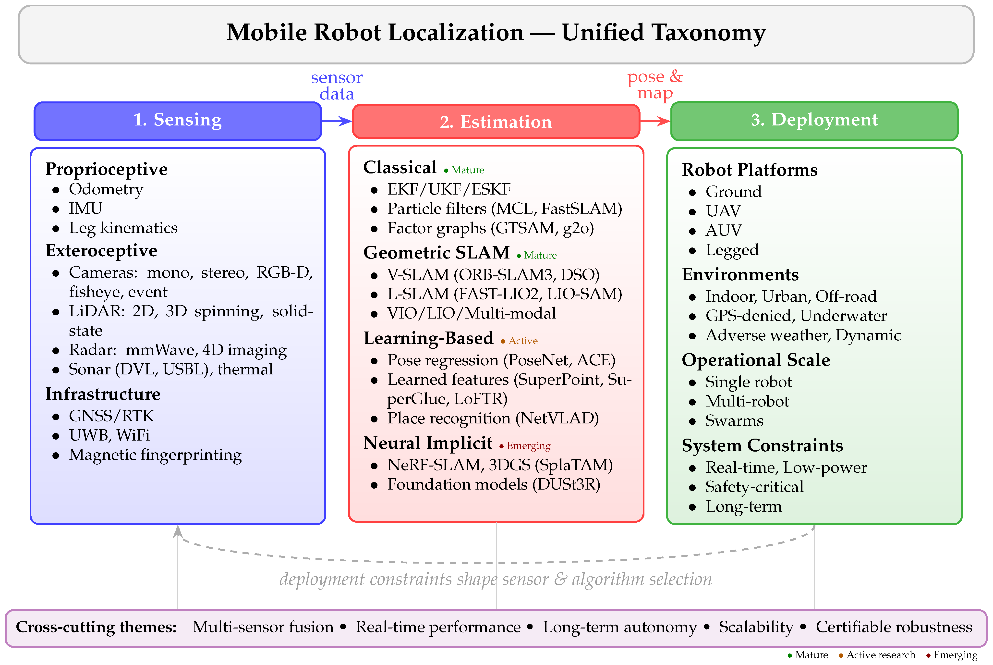
Figure 1 provides a unified visual taxonomy of the three interconnected pillars (sensing modalities, estimation paradigms, and deployment contexts) that structure this review, together with the forward data-flow pipeline and the feedback arc by which deployment constraints shape sensor and algorithm selection.

2. Methodology of the Review

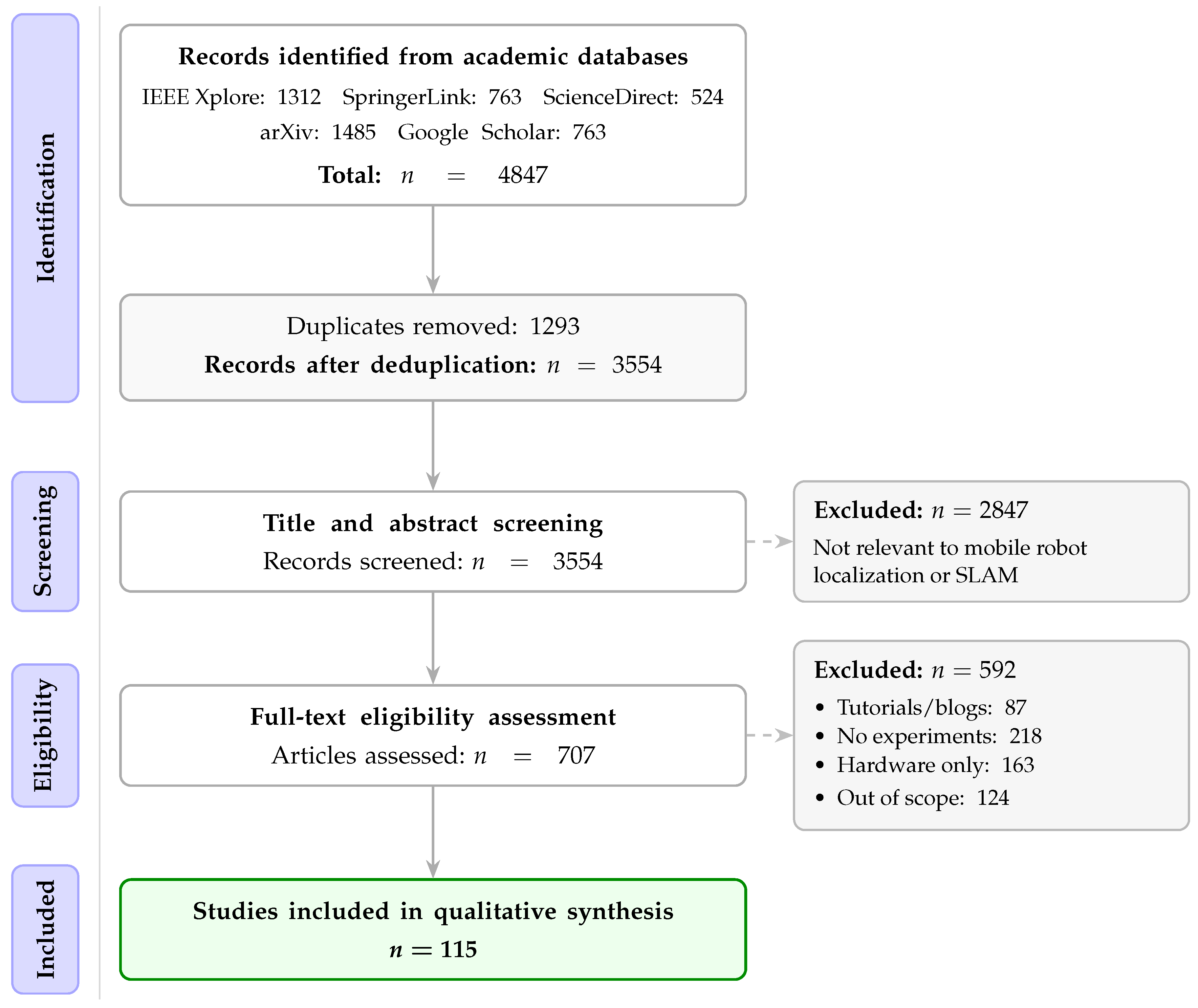
This survey provides a critical and up-to-date review of localization and SLAM technologies spanning classical probabilistic methods, geometric multi-sensor systems, and emerging learning-based paradigms. Rather than cataloging developments descriptively, our goal is to expose the state of the art honestly, identifying what works, where significant gaps remain, and why achieving a truly unified and deployable localization system is harder than the literature often suggests. To ensure reproducibility and transparency, this review followed a structured literature selection and classification methodology in strict accordance with the PRISMA 2020 reporting guidelines [19]. A completed PRISMA flow diagram is included in Section 2.5 (Figure 2), and the completed PRISMA 2020 checklist is provided in the Supplementary Materials.

Regarding the review protocol, this systematic review was not prospectively registered in a public registry such as PROSPERO or INPLASY, as it focuses on algorithmic and hardware evaluation in robotics rather than health or social care interventions.

2.1. Search Strategy

Publications were collected from five academic databases covering the period January 1990 to January 2026: IEEE Xplore, SpringerLink, ScienceDirect, arXiv, and Google Scholar. The core Boolean query applied to title, abstract, and keyword fields was as follows:

(“SLAM” OR “simultaneous localization and mapping” OR “mobile robot localization”) AND (“LiDAR” OR “visual odometry” OR “IMU fusion” OR “neural SLAM” OR “NeRF” OR “Gaussian splatting” OR “deep learning” OR “sensor fusion” OR “place recognition” OR “radar odometry”)

Database-specific syntax adaptations were applied as needed (e.g., field tags TI:, AB:, KW: on IEEE Xplore; title-abs-key() on ScienceDirect). These queries yielded 4847 records in total (IEEE Xplore: 1312; SpringerLink: 763; ScienceDirect: 524; arXiv: 1485; Google Scholar: 763), spanning publications from 1990 to January 2026. The complete per-database Boolean strings are provided in Supplementary Material S1.

Retrieval dates and language restriction. All database queries were executed between 7 and 23 January 2026, with the Google Scholar citation cross-checks completed last within this window, and the record counts reported above correspond to these retrieval dates. The search was restricted to publications written in English. No other language filters were applied. We acknowledge that this restriction may introduce a language bias by under-representing contributions published exclusively in other languages, although the overwhelming majority of archival robotics literature in the surveyed venues is published in English.

Screening harmonization. Title/abstract screening and full-text eligibility assessment were performed independently and in duplicate by two reviewers (J.M.G.H. and R.P.-R.). Before formal screening, both reviewers completed a calibration pilot on a random sample of 200 records, jointly refining the interpretation of each inclusion and exclusion criterion until the criteria could be applied consistently; the pilot records were then re-screened under the harmonized rules. During formal screening, conflicting decisions were first resolved by discussion between the two reviewers, and persistent disagreements were arbitrated by a third senior reviewer (F.M.R.). All screening decisions, together with the reason for each full-text exclusion, were recorded in a shared spreadsheet to preserve an auditable trail of the selection process.

Preprint policy. arXiv preprints were included in the initial retrieval to avoid systematic exclusion of recent contributions not yet formally published. However, a preprint was retained in the final corpus only if no peer-reviewed version was available and the work represented a substantive algorithmic or empirical contribution independently cited by ≥5 peer-reviewed papers. Preprints meeting this criterion are identified with the tag [preprint] in Supplementary Material S2.

2.2. Inclusion Criteria

The primary analytical unit of this review is a localization or SLAM contribution: a work was eligible for inclusion if it either (a) proposed a novel algorithm, representation, or sensor modality whose primary output is a robot pose or map, or (b) provided an evaluation dataset or metric directly used to assess such systems. To maintain a coherent synthesis, survey-only contributions (without an algorithmic or dataset contribution) and deployment reports (without a quantitative localization evaluation) were categorized separately and are cited as context rather than included in the risk-of-bias assessment (Section 2.4). Papers satisfying this primary criterion were further required to meet all of the following criteria:

• Reported at least one quantitative localization or mapping metric (ATE, RPE, RMSE, Recall@N, or equivalent);
• Evaluated on a platform that physically moved through an environment (ground vehicle, UAV, AUV, legged robot, or hand-held rig);
• Were peer-reviewed or, for preprints, met the citation threshold defined in Section 2.1.

Where multiple papers addressed the same contribution, preference was given to the most recent peer-reviewed version and to works published between 2015 and 2025. Papers outside this range were retained when they represented foundational contributions with ≥100 citations in Google Scholar (verified January 2026), ensuring reproducibility of the selection decision.

2.3. Exclusion Criteria

The following works were excluded:

• Non-peer-reviewed blog posts or tutorials;
• Papers without experimental validation;
• Works focused exclusively on hardware design without a localization or mapping contribution.

Note: arXiv preprints are not excluded by this criterion. They are governed separately by the preprint policy in Section 2.1 and retained only when the conditions stated there are met.

2.4. Quality Assessment and Risk of Bias

Following PRISMA 2020 item 12 [19] and adapting the QUADAS-2 quality appraisal structure [20] to the computational robotics domain, each of the 115 retained papers (those satisfying both the localization-contribution requirement and all three quantitative inclusion criteria) was assessed for risk of bias across five dimensions:

• Reproducibility (weight $w_1=0.25$): Source code or evaluation data openly released, or results independently replicated on a public benchmark by a third party.
• Dataset independence (weight $w_2=0.20$): Primary evaluation performed on at least one public benchmark not used for algorithm design or hyperparameter tuning.
• Ablation completeness (weight $w_3=0.20$): Key design choices individually ablated, or equivalent sensitivity analysis provided.
• Real-world validation (weight $w_4=0.20$): System tested on a physical robot platform under conditions beyond a controlled laboratory.
• Uncertainty reporting (weight $w_5=0.15$): Trajectory error or performance metrics accompanied by variance or confidence intervals across multiple runs or evaluation sequences.

Scoring and aggregation. Each dimension was scored as 0 (High risk), 0.5 (Moderate risk), or 1 (Low risk) by two independent reviewers (J.M.G.H. and R.P.-R.), with disagreements resolved by discussion. This quality appraisal is a separate stage from, and downstream of, the study-selection screening described in Section 2.1, and was applied only to the 115 papers already retained by that screening. The aggregate risk score for paper k is $S_k={\sum }_{i=1}^5{w}_i{s}_{ki}$, where $s_{ki}$ is the score on dimension i. Papers with $S_k<0.40$ are designated High overall risk and their quantitative claims are treated with higher skepticism in subsequent sections; those with $0.40\le S_k<0.70$ are Moderate; and those with $S_k\ge 0.70$ are Low. The dimension weights were chosen to prioritize reproducibility, as this is the primary barrier to independent verification in computational robotics; the rationale follows recommendations in Amrhein et al. [21].

Inter-rater agreement. Because a single pooled agreement statistic can mask materially different reviewer reliability across quality dimensions, Cohen’s $\kappa$ was computed separately for each of the five dimensions in addition to the pooled value. Agreement was highest for the two dimensions with the most objectively verifiable evidence, reproducibility ($\kappa =0.82$, near-perfect), and real-world validation ($\kappa =0.79$, substantial), followed by dataset independence ($\kappa =0.76$, substantial). Agreement was lower, though still substantial, for the two dimensions requiring more interpretative judgment: uncertainty reporting ($\kappa =0.68$) and ablation completeness ($\kappa =0.66$), where reviewers occasionally differed on whether partial ablations or single-sequence variance figures satisfied the criterion. The pooled agreement across all $115\times 5$ judgments was $\kappa =0.74$ (substantial agreement per Landis & Koch [22]). All disagreements, which were concentrated in the two lower-agreement dimensions, were resolved by discussion before aggregation, so the scores entering $S_k$ reflect consensus judgments.

The key finding from this assessment is that only 34% of the 115 retained papers (i.e., 39 papers, identified individually in Supplementary Material S2, Table S5) reported variance statistics across multiple evaluation runs. The corpus-wide risk-of-bias counts across all five quality dimensions are summarized in Supplementary Table S2, while

Table 1. Risk-of-bias summary (papers scored Moderate or High risk, i.e., $s_{ki}\le 0.5$) disaggregated by algorithmic paradigm, aggregated across the 115-paper corpus. Cells report the numerator count over the subgroup size, the corresponding percentage, and the 95% Wilson score confidence interval in brackets. The intervals for the NeRF-SLAM ($n=15$) and 3DGS-SLAM ($n=10$) subgroups are wide, reflecting their small sample sizes; percentage-point differences between these two subcategories should therefore not be over-interpreted, whereas their separation from the LiDAR and Visual SLAM subgroups exceeds the interval overlap on real-world validation. The full five-dimension breakdown is provided in Supplementary Material S2, Table S3.

Dimension	Visual SLAM	LiDAR SLAM	NeRF-SLAM	3DGS-SLAM	Multi-robot
(Moderate/High)	($\mathit{n}=\mathbf{41}$)	($\mathit{n}=\mathbf{32}$)	($\mathit{n}=\mathbf{15}$)	($\mathit{n}=\mathbf{10}$)	($\mathit{n}=\mathbf{17}$)
Reproducibility	14/41, 34% [22–49]	7/32, 22% [11–39]	8/15, 53% [30–75]	5/10, 50% [24–76]	7/17, 41% [22–64]
Real-world validation	16/41, 39% [26–54]	7/32, 22% [11–39]	14/15, 93% [70–99]	8/10, 80% [49–94]	10/17, 59% [36–78]
Uncertainty reporting	24/41, 59% [43–72]	17/32, 53% [36–69]	14/15, 93% [70–99]	9/10, 90% [60–98]	12/17, 71% [47–87]

disaggregates the two most decision-relevant dimensions by algorithmic paradigm, reporting for each cell the underlying numerator count and a 95% Wilson score confidence interval alongside the percentage; Supplementary Material S2 (Table S3) provides the full five-dimension breakdown by paradigm. The per-dimension inter-rater agreement statistics are reported in Supplementary Table S1, and the complete per-paper score sheet is available from the corresponding author on request.

NeRF-based and 3DGS-based SLAM carry substantially higher risk than classical LiDAR or visual SLAM on every dimension, most acutely on real-world validation and uncertainty reporting, while LiDAR SLAM carries the lowest overall risk, benefiting from mature open benchmarks and a strong culture of open-source release.

Sensitivity of the paradigm ranking to the dimension weights. Because the weights $w_1,\dots ,w_5$ were fixed a priori, we verified that the qualitative conclusions drawn from the risk assessment do not hinge on this particular choice. For each paradigm we computed a weighted risk index, defined as the weight-averaged share of papers that scored Moderate or High across the five dimensions, under five plausible weighting schemes: the baseline weights above; uniform weights ($w_i=0.20$ for all i); and three single-dimension-dominant schemes in which one dimension receives $w=0.40$ and the remaining four share the residual equally ($w=0.15$), successively emphasizing reproducibility, real-world validation, and uncertainty reporting.

Table 2. Sensitivity of the paradigm-level risk ordering to the dimension weights. Each cell is the weighted risk index (weight-averaged % of papers scored Moderate or High across the five dimensions of Supplementary Table S3) under the indicated weighting scheme. Lower is better. The rank order is identical in every row.

Weighting Scheme	LiDAR	Visual	Multi-Robot	3DGS	NeRF
Baseline ($0.25/0.20/0.20/0.20/0.15$)	31.6	39.7	59.7	66.0	72.6
Uniform ($w_i=0.20$)	33.1	41.0	61.2	68.0	74.6
Reproducibility-dominant ($w_1=0.40$)	30.3	39.2	56.2	63.5	69.2
Validation-dominant ($w_4=0.40$)	30.3	40.5	60.6	71.0	79.2
Uncertainty-dominant ($w_5=0.40$)	38.1	45.3	63.5	73.5	79.2

reports the resulting indices (reproduced in Supplementary Table S4). The ordering of the five paradigms, LiDAR SLAM < Visual SLAM < Multi-robot < 3DGS-SLAM < NeRF-SLAM (from lowest to highest risk), is identical under all five schemes, and the separation between the geometric paradigms (LiDAR; Visual) and the neural subcategories (NeRF; 3DGS) exceeds 20 percentage points in every scheme. The paradigm-level conclusions of this review are therefore robust to plausible alternative weightings; the weights affect the magnitude of the aggregate scores $S_k$ but not the relative ranking on which the interpretative claims rest. Only the adjacent pair Multi-robot vs. 3DGS-SLAM narrows appreciably (to within roughly 7 points) under the reproducibility-dominant scheme, and even there the ordering is preserved.

This motivates the closer scrutiny applied to neural SLAM claims throughout Section 8 and Section 12: claims from neural SLAM papers are treated as benchmark-only findings rather than validated deployment performance unless corroborated by independent reproduction or field results, and the FPS and convergence-time figures discussed below (Section 12) should be read with the 93%/80% real-world-validation risk of their source subcategories in mind.

2.5. Taxonomy Construction

The final taxonomy was designed to bridge classical probabilistic robotics and modern learning-based approaches. The literature was categorized along three axes:

• Sensor modality;
• Algorithmic paradigm;
• Deployment scale (single vs multi-robot).

After removing 1293 duplicates, 3554 records were screened by title and abstract. Of these, 707 full-text articles were assessed for eligibility. Applying the inclusion and exclusion criteria described above, a total of 115 publications were retained for qualitative synthesis. The complete selection process is illustrated in Figure 2.

The retained corpus informs each thematic axis of this review: sensor modalities and fusion are analyzed in Section 4, classical probabilistic estimation is analyzed in Section 6, modern SLAM frameworks are analyzed in Section 7 and Section 8, deep-learning-based localization is analyzed in Section 9, and multi-robot collaborative SLAM is analyzed in Section 10. Of the 115 retained papers, 54 (47%) are camera-based, 43 (37%) are LiDAR-based, and 31 (27%) are multi-modal; ground vehicles account for 45% of platforms, and 68% of systems are real-time capable. Sensor-modality counts are deliberately non-exclusive and therefore overlap: the coding rule assigns each paper to every sensor-modality category whose data it consumes for state estimation, and additionally to the multi-modal fusion category when two or more exteroceptive modalities are tightly or loosely coupled in a single estimator. For example, a LiDAR–visual-inertial system such as LVI-SAM is counted once under visual/camera-based, once under LiDAR-based, and once under multi-modal fusion. Consequently, the five modality subcategories (54 visual/camera-based, 43 LiDAR-based, 31 multi-modal fusion, 23 learning-based/neural, and 10 other-sensor (sonar, radar, and UWB)) sum to 161 assignments across the 115 papers (full breakdown in Supplementary Table S6), and the percentages (which are computed over the 115-paper corpus) sum to more than 100%. The robotic-platform categories, by contrast, are mutually exclusive and sum to the 115-paper corpus (Supplementary Table S6), whereas the operational-mode categories are, like the sensor modalities, non-exclusive and therefore do not sum to 115. Sensor modality, algorithmic paradigm, and robotic platform are independent classifications, so their per-category counts are not directly comparable across axes: the visual/camera-based modality count (54) exceeds the Visual SLAM paradigm count (41 in Table 1) because many LiDAR- and fusion-paradigm systems also consume camera data, and the neural paradigms (NeRF-SLAM and 3DGS-SLAM, 25 papers combined) need not equal the learning-based/neural modality tally (23), since a neural system running on RGB-D input is additionally counted under the visual modality. The full thematic distribution across sensor modality, robotic platform, and operational mode is provided in Supplementary Material S3.

3. Comparison with Existing Surveys

Prior surveys of SLAM and localization typically focus on a single paradigm. Cadena et al. [2] remains the primary reference for classical SLAM. Bresson et al. [23] focused on autonomous driving. Fuentes-Pacheco et al. [24] surveyed visual SLAM from direct to feature-based methods. Chen et al. [25] extended coverage to deep-learning localization (pose regression, scene coordinates, and learned features). Tosi et al. [18] most recently reviewed NeRF and 3D Gaussian Splatting within SLAM.

Table 3. Comparison with representative surveys in SLAM and localization.

Survey	Year	Sensors	Classical SLAM	Deep Learning	Multi-Robot	Cross-Domain
Fuentes-Pacheco et al. [24]	2015	Vision	Yes	No	No	No
Cadena et al. [2]	2016	Yes	Yes	No	Yes	No
Bresson et al. [23]	2017	Yes	Yes	No	No	No
Chen et al. [25]	2020	Yes	Yes	Yes	No	No
Tosi et al. [18]	2024	Vision	No	Yes	No	No
This survey	2026	Yes	Yes	Yes	Yes	Yes

summarizes their scope against this work.

Unlike any prior survey, this work bridges classical probabilistic estimation, geometric multi-sensor SLAM, neural and learning-based representations, multi-robot collaboration, and cross-domain deployment challenges within a single unified framework. The motivating insight is that no single paradigm addresses all facets of the problem: a complete understanding of mobile robot localization requires traversing the full stack from sensor physics to system deployment. The next section begins that journey by examining the sensory hardware that underpins every localization pipeline.

4. Sensor Suites Across Robotic Domains

The foundation of any localization system relies on its sensory input. The choice of sensors is highly dependent on the robot’s payload capacity, power constraints, computational budget, and operating environment. This section provides a comprehensive overview of the main sensor categories.

4.1. Proprioceptive Sensors

Proprioceptive sensors measure internal state without reference to the environment. Wheel encoders and leg kinematics provide high-frequency (>100 Hz), low-cost displacement estimates via kinematic models but accumulate unbounded drift from slippage and terrain effects [3,26]. IMUs (accelerometer + gyroscope, often with magnetometer) range from lightweight consumer-grade MEMS units with significant bias instability to costlier tactical/navigation-grade units with far lower drift [27]. IMU preintegration [28] is now the standard technique for incorporating IMU data into optimization-based SLAM backends.

4.2. Exteroceptive Sensors

Exteroceptive sensors measure the robot’s relationship to its external environment and are essential for bounding the drift inherent in proprioceptive sensing.

4.2.1. Vision Sensors (Cameras)

Monocular cameras are cheap and information-rich but cannot recover metric scale without auxiliary information [10,29]. Stereo pairs resolve scale via triangulation at the cost of a baseline-limited depth range [30]. RGB-D cameras give per-pixel depth but are limited to indoor use and short range (<10 m) [31]. Wide-field and fisheye lenses reduce tracking loss during fast rotation, benefiting UAVs and legged robots [32]. Event cameras (DVS) report asynchronous per-pixel brightness changes with microsecond latency, high dynamic range (>120 dB), and low power draw, suiting high-speed and low-light operation [33], as demonstrated by EVO [34] and Ultimate SLAM [35].

4.2.2. LiDAR (Light Detection and Ranging)

Two-dimensional LiDARs have long served indoor navigation via occupancy-grid mapping and MCL [1]. Three-dimensional spinning LiDARs provide dense point clouds at 10–20 Hz and remain the standard for autonomous driving, at the cost of weight (0.5–1.5 kg) and power (8–20 W) [36]. Solid-state LiDARs offer a lighter, cheaper, mechanically simpler alternative, though their non-repetitive scan patterns have required purpose-built algorithms such as FAST-LIO2 [12].

4.2.3. Radar

mmWave FMCW radar (77–79 GHz) is robust to rain, fog, dust, and snow where cameras and LiDAR degrade. Modern 4D imaging radars add dense point clouds with simultaneous Doppler velocity, enabling radar SLAM [37,38]. Scanning radar produces 360° range-azimuth images usable for place recognition even with zero optical visibility [39].

4.2.4. Acoustic and Sonar Sensors

Underwater, electromagnetic attenuation makes acoustic sensing dominant. DVLs measure seafloor-relative velocity for the dead-reckoning core of most AUV navigation stacks [40]. USBL/SBL/LBL acoustic positioning gives absolute fixes from centimeters (LBL) to a few meters (USBL) depending on configuration [41]. Side-scan and multibeam sonar support terrain-relative navigation and underwater SLAM [42].

4.2.5. Thermal Cameras

LWIR thermal cameras (8–14 µm) enable operation in darkness, smoke, and visually degraded scenes and have been explored for search-and-rescue and night-time driving [43], though low contrast and day/night “thermal crossover” complicate long-term place recognition.

4.3. Global and Infrastructure-Based Sensors

GNSS gives absolute position (2–5 m standalone; centimeter-level with RTK/PPP) but is unreliable indoors, underwater, in urban canyons, and under forest canopy [44]. UWB ranging achieves centimeter accuracy via time-of-flight but needs pre-deployed anchors and is sensitive to NLOS errors [45]. WiFi fingerprinting gives coarse (2–5 m) infrastructure-free indoor localization [46], while geomagnetic fingerprinting can reach 0.5–1.5 m via learned regression, at the cost of per-platform calibration and sensitivity to field changes of up to 30% within weeks [47].

4.4. Sensor Comparison Summary

Table 4. Comparison of principal sensor modalities for mobile robot localization. Each row cites the primary reference used to document the reported specifications; cost ranges are indicative market prices from manufacturer datasheets (accessed January 2026) and vary by vendor and configuration.

Sensor	Range	Precision	Rate	Weight	Env.	Cost (USD)
Wheel Encoder [3]	–	mm	>100 Hz	Low	Ground	$10–200
IMU (MEMS) [27]	–	Variable	200–1000 Hz	Low	All	$20–200
Monocular Cam. [10,29]	∞	px-level	30–120 Hz	Very Low	Lit	$50–500
Stereo Camera [30]	0.5–20 m	cm	30–90 Hz	Low	Lit	$200–800
RGB-D Camera [31]	0.3–10 m	mm–cm	30 Hz	Low	Indoor	$100–500
Event Camera [33]	∞	px-level	µs	Very Low	All	$3k–15k
2D LiDAR [1]	0.1–30 m	cm	10–40 Hz	Low	All	$100–2k
3D LiDAR [36]	0.3–200 m	cm	10–20 Hz	Medium	All	$5k–80k
Solid-State LiDAR [12]	0.3–450 m	cm	10 Hz	Low	All	$1k–10k
4D Imaging Radar [37,38]	0.2–300 m	dm	10–20 Hz	Low	All	$2k–20k
DVL [40]	0.5–200 m	mm/s	1–10 Hz	Medium	Underwater	$5k–30k
USBL [41]	100–10,000 m	0.1–1% R	0.1–1 Hz	Medium	Underwater	$5k–60k
Thermal Camera [43]	∞	px-level	30–60 Hz	Low	All	$1k–10k
GNSS (RTK) [44]	Global	cm	1–20 Hz	Low	Outdoor	$500–5k
UWB [45]	0–100 m	cm–dm	10–100 Hz	Very Low	Indoor	$30–200

provides a comprehensive comparison of the principal sensor modalities used for mobile robot localization, covering accuracy, range, update rate, weight, operational environment, and cost.

The complementary strengths and weaknesses of sensing hardware make the choice of estimation algorithm equally critical. Before examining these algorithms in detail, however, it is important to understand how their performance is measured in practice. The following section surveys the standard benchmark datasets and evaluation metrics used throughout this review.

5. Benchmark Datasets and Evaluation

Standardized benchmarks are essential for fair comparison of localization algorithms.

Table 5. Principal benchmark datasets for mobile robot localization and SLAM evaluation. The last two columns characterize the evaluation contract of each dataset: the ground-truth modality with its indicative accuracy, and the trajectory metric with its canonical alignment protocol (Umeyama SE(3)/Sim(3) alignment for ATE-based protocols; segment-wise relative errors without global alignment for KITTI-style protocols). Because these contracts differ, error figures are not directly comparable across datasets (see discussion below).

Dataset	Sensors	Environment	Ground Truth (Accuracy)	Metric/Alignment	Ref.
KITTI Odometry	Stereo, LiDAR, GPS/IMU	Outdoor driving	RTK-GNSS/INS (∼10 cm)	RTE/RRE, per-segment, no align.	[48]
EuRoC MAV	Stereo, IMU	Indoor MAV	Laser tracker/Vicon (mm)	ATE, SE(3) Umeyama	[49]
TUM RGB-D	RGB-D	Indoor handheld	Motion capture (mm)	ATE/RPE, SE(3)/Sim(3)	[31]
TUM VI	Stereo, IMU	Indoor/outdoor	Mocap (partial coverage)	ATE on mocap segments	[50]
nuScenes	Camera, LiDAR, Radar	Urban driving	Map-based loc. + GNSS/INS (dm)	Task-specific (detection-centric)	[51]
Hilti Challenge	LiDAR, Camera, IMU	Construction sites	Total station/TLS prisms (mm–cm)	ATE at control points, SE(3)	[52]
M2DGR	Multi-modal	Ground robot	RTK-GNSS/mocap/tracker (cm)	ATE, SE(3) Umeyama	[53]
Oxford RobotCar	Camera, LiDAR, GPS	Urban long-term	GPS/INS (m-level, drifting)	RTE/place-recognition recall	[54]
Newer College	LiDAR, Camera, IMU	Outdoor handheld	ICP vs. TLS prior map (cm)	ATE, SE(3) Umeyama	[55]
SubT-MRS	Multi-modal	Subterranean	Total station + FARO scans (cm)	ATE, SE(3); failures logged	[56]

summarizes the most widely used datasets.

Evaluation metrics typically include Absolute Trajectory Error (ATE) and Relative Pose Error (RPE), as formalized by Sturm et al. [31]. The EVO evaluation toolbox [57] has become the standard tool for computing these metrics.

The benchmark inventory in Table 5 distinguishes four properties that are frequently conflated when results are compared across datasets. First, the ground-truth modality bounds the smallest error that can meaningfully be reported: sub-centimeter ATE claims are interpretable against millimeter-accurate motion capture (EuRoC; TUM RGB-D) but not against meter-level GPS/INS references (Oxford RobotCar), and datasets with partial ground-truth coverage (TUM VI) evaluate only the covered segments. Second, the trajectory alignment protocol changes what an error number means: EuRoC- and TUM-style ATE is computed after a global SE(3) (or, for monocular systems, Sim(3)) Umeyama alignment, which absorbs any global offset and, in the Sim(3) case, scale drift, whereas the KITTI protocol reports segment-wise relative translation and rotation errors over 100–800 m sub-paths without any global alignment, penalizing local drift but not loop-closure consistency. Third, failure handling differs silently across benchmarks: most leaderboards report errors only over the frames for which the system produced a pose, so sequences with tracking loss either disappear from the statistics or are excluded altogether, a practice that motivates the Trajectory Completeness metric proposed in Section 13. Fourth, sequence difficulty is heterogeneous both across and within datasets: EuRoC spans deliberately stratified easy-to-difficult sequences (MH_01 vs. V2_03), the Hilti Challenge and SubT-MRS are constructed to induce degraded perception, and driving datasets differ in dynamic-object density and route length. For all four reasons, ATE and RPE figures are directly comparable only within a single dataset under a declared alignment protocol and failure-handling rule. Cross-dataset comparisons in this review are therefore stated as qualitative rankings rather than pooled numeric averages, and every quantitative figure cited in later sections is tied to its source benchmark.

A comprehensive comparison of representative SLAM systems across sensor modalities, including their backend, real-time capability, loop closure support, and open-source availability, is provided in

Table 6. Representative SLAM systems comparison.

System	Sensor	Real-Time	Loop Closure	GPU	Open-Source	Environment
ORB-SLAM3	Mono/Stereo/VIO	Yes	Yes	No	Yes	Indoor/Outdoor
Cartographer	LiDAR	Yes	Yes	No	Yes	Indoor/Outdoor
LOAM	LiDAR	Yes	Limited	No	Yes	Outdoor
VINS-Fusion	VIO	Yes	Yes	No	Yes	Indoor/Outdoor
LIO-SAM	LiDAR+IMU	Yes	Yes	No	Yes	Outdoor
Kimera	VIO	Yes	Yes	Optional	Yes	Indoor

.

With this evaluation framework established, the following section traces the evolution of probabilistic estimation, the mathematical bedrock on which all modern localization systems are constructed.

6. Classical Probabilistic State Estimation

Before the widespread adoption of SLAM, localization was conceived as a pure probabilistic state estimation problem, and the elegant mathematical framework that emerged from this era still underpins every competitive modern system. Understanding these foundations is not merely historical: Bayesian filtering, particle methods, and factor graph optimization remain the computational backbone of the best-performing SLAM pipelines available today, including those that incorporate deep learning components. The core formalism is the Recursive Bayes Filter, which estimates the belief of the robot’s state $x_t$ given the history of controls $u_{1:t}$ and observations

$z_{1:t}$ [1]:

$$bel\left(x_t\right)=\eta p(z_t\mid x_t)\int p(x_t\mid u_t,x_{t-1})bel\left(x_{t-1}\right)d{x}_{t-1},$$

(1)

where

• $bel\left(x_t\right)=p(x_t\mid z_{1:t},u_{1:t})$ is the belief—the posterior probability distribution over robot state $x_t$ given all past observations and controls;
• $\eta$ is a scalar normalization constant ensuring the posterior integrates to unity;
• $p(z_t\mid x_t)$ is the observation likelihood (sensor or measurement model), giving the probability of receiving measurement $z_t$ if the true state is $x_t$;
• $p(x_t\mid u_t,x_{t-1})$ is the motion model (state-transition density), encoding the probability of transitioning from $x_{t-1}$ to $x_t$ under control input $u_t$.

Practical implementations of this formulation differ primarily in how they represent the belief distribution $bel\left(x_t\right)$.

6.1. Gaussian Filters

When belief is well-approximated by a unimodal Gaussian, parametric filters are computationally efficient. The EKF linearizes nonlinear motion/observation models via first-order Taylor expansion; it remains widely used for pose tracking and loosely coupled sensor fusion, though linearization can cause inconsistency in highly nonlinear systems [58]. The UKF instead propagates mean and covariance via deterministic sigma-point sampling, achieving second-order accuracy without explicit Jacobians and outperforming the EKF under strong nonlinearity [58]. The ESKF estimates the error between the predicted and true state rather than the full state, avoiding quaternion singularities and improving numerical stability; it is the standard for IMU-centric navigation [59]. The IEKF, used in systems such as FAST-LIO2 [12], iteratively re-linearizes the observation model within each update, improving accuracy in strongly nonlinear cases such as point-to-plane LiDAR registration.

6.2. Particle Filters (Monte Carlo Localization)

Multi-modal or highly non-Gaussian beliefs, as in global localization or kidnapped-robot recovery, require non-parametric representations. Standard MCL represents belief as weighted particles updated via sequential importance sampling and resampling [6], refined into Adaptive MCL with KLD-sampling that adjusts particle count to posterior complexity [7]. Rao-Blackwellized particle filters exploit the SLAM posterior’s factorization into a particle filter over trajectories and independent Gaussian filters over landmarks: FastSLAM [60] introduced this, achieving far better scalability than monolithic EKF-SLAM, and GMapping [61] extended it to grid maps, substantially reducing the computational cost of particle-filter SLAM indoors.

6.3. Graph-Based Optimization (Factor Graphs)

Filter-based methods cannot revisit past estimates after loop closure, motivating smoothing-based methods that formulate SLAM as nonlinear least-squares over all past poses and landmarks [62,63]. iSAM/iSAM2 uses a Bayes-tree structure for incremental, just-in-time relinearization, enabling real-time full SLAM without re-solving from scratch [63]. GTSAM is the de facto standard factor-graph library underlying numerous SLAM systems [64]. Ceres Solver [65] and g2o [66] are complementary optimization backends offering efficient Levenberg-Marquardt and Gauss-Newton implementations widely used in visual and LiDAR SLAM.

6.4. Key Insights: Classical Estimation

• Classical probabilistic methods provide the principled uncertainty quantification that learning-based systems largely lack, with serious consequences for safety-critical deployment.
• No purely classical method has demonstrated reliable long-term autonomy in environments that change over time. This limitation motivates the multi-sensor and learning-augmented SLAM systems reviewed in the following section.

The limitations of classical filtering and graph-based SLAM become most apparent when a robot must build and maintain a map in real time across diverse sensor modalities and continuously changing environmental conditions. The following section examines how the SLAM community has addressed these demands through specialized frameworks organized by sensing paradigm.

7. Modern Simultaneous Localization and Mapping (SLAM)

Simultaneous localization and mapping (SLAM) represents the culmination of classical probabilistic theory applied to the joint pose-and-environment estimation problem. Over the past decade, algorithmic progress has been remarkable: open-source systems such as ORB-SLAM3, FAST-LIO2, and VINS-Fusion now achieve centimeter-level accuracy on standard benchmarks with commodity hardware. Yet this apparent maturity is deceiving. Despite remarkable progress, current SLAM systems still struggle with long-term autonomy and dynamic environments, two requirements that are non-negotiable for real-world deployment but conspicuously absent from most benchmark evaluations. This section reviews the major SLAM paradigms organized by sensing modality, explicitly highlighting where each approach excels and where it breaks down.

Table 6 summarizes widely used SLAM systems across sensor modalities and deployment scenarios.

7.1. Visual SLAM (V-SLAM)

Visual SLAM systems use cameras as their primary sensor and can be broadly categorized into feature-based (indirect) and direct methods.

Feature-based methods extract sparse keypoints, match them across frames, and minimize reprojection error. MonoSLAM [67] was the first real-time monocular SLAM system (EKF-based). PTAM [9] introduced parallel tracking/mapping threads and keyframe bundle adjustment, patterns that persist today. The ORB-SLAM family [10,30,32] is the most complete and widely used open-source visual SLAM library; ORB-SLAM3 supports mono/stereo/RGB-D/fisheye/visual-inertial configurations, with DBoW2-based place recognition [68], an Atlas multi-map system, and a tightly coupled visual-inertial MAP backend.

Direct methods minimize photometric error over raw pixels rather than sparse keypoints, exploiting edges and gradients in weakly textured regions. LSD-SLAM [69] pioneered semi-dense direct monocular SLAM. DSO [29] combines sparse selection of high-gradient points with joint optimization of depth, pose, and photometric parameters; its stereo extension [70] recovers metric scale. SVO [71] hybridizes direct frame-to-frame tracking with a feature-based backend, originally for MAVs.

7.2. Visual-Inertial Odometry and SLAM (VIO/VI-SLAM)

Camera-IMU fusion is the dominant paradigm for UAV and mobile-device localization: IMUs supply metric scale and bridge visual tracking failures, while cameras bound IMU drift. MSCKF [72] is an efficient filter-based VIO marginalizing tracked features as multi-state constraints (successors include OpenVINS [73]). OKVIS [74] was among the first tightly coupled keyframe-based optimization VIO systems with IMU preintegration factors. VINS-Mono/VINS-Fusion [75,76] is a widely benchmarked tightly coupled monocular VIO system with robust initialization, online extrinsic calibration, 4-DoF pose-graph loop closure, and (in VINS-Fusion) GNSS fusion. Kimera [77] extends metric-semantic SLAM to real-time 3D mesh and semantic mapping. BASALT [78] achieves state-of-the-art EuRoC accuracy via non-linear factor recovery while remaining real-time.

7.3. LiDAR SLAM and LiDAR-Inertial Odometry (LIO)

LiDAR SLAM exploits precise geometric range measurements. LOAM [36] is the foundational algorithm, separating high-frequency/low-fidelity odometry from low-frequency/high-fidelity mapping via edge/planar feature registration; its KITTI performance set the standard for later work. Cartographer [79] (Google) supports 2D/3D LiDAR with optional IMU, using scan-to-submap matching and pose-graph loop closure, and is a common ROS baseline in service/warehouse robotics. LeGO-LOAM [80] is a lightweight, ground-optimized variant for embedded ground vehicles. LIO-SAM [11] is a factor-graph (GTSAM) system fusing IMU, LiDAR odometry, GPS, and loop-closure factors and is among the most widely adopted LiDAR SLAM systems. FAST-LIO/FAST-LIO2 [12,81] use an Iterated EKF with an incremental k-d tree (ikd-Tree) for real-time map maintenance, achieving state-of-the-art accuracy while running on embedded ARM processors, making it suitable for payload-constrained UAVs. Point-LIO [82] extends this paradigm to per-point (rather than per-scan) state estimation for robustness under aggressive motion. KISS-ICP [83] is a minimalist point-to-point ICP odometry system that is competitive across diverse platforms without an IMU or extensive tuning, showing that well-engineered classical methods remain viable.

7.4. Radar SLAM

Radar’s weather robustness has driven growing interest in radar-based localization. Scanning-radar odometry (Navtech-based) demonstrates place recognition and metric localization in fog and heavy rain where camera/LiDAR fail entirely, with ring-key descriptors enabling robust loop closure [39]. Four-dimensional imaging radar, providing dense point clouds with per-point radial velocity, enables systems such as 4DRadarSLAM [38] and EKF-based radar-inertial odometry [37] approaching LiDAR-level accuracy in some scenarios.

7.5. Multi-Modal SLAM

State-of-the-art systems increasingly fuse multiple exteroceptive sensors. LVI-SAM [84] tightly couples LiDAR, vision, and inertial data, with VIO seeding LiDAR scan matching and LiDAR depth initializing visual features, degrading gracefully if either subsystem fails. R3LIVE [85] combines an IEKF-based LiDAR-inertial subsystem with a photometric visual-inertial subsystem, yielding both accurate odometry and colored 3D reconstruction. FAST-LIVO [86] extends FAST-LIO2 with direct visual odometry in a single IEKF, improving robustness where visual or geometric features are scarce.

7.6. Key Insights: SLAM Paradigms

• Tightly coupled multi-sensor fusion (LiDAR+camera+IMU) represents the current state of the art in robustness, but introduces calibration complexity and single points of failure at the fusion interface.
• Despite decades of research, no existing SLAM system has demonstrated sustained reliable operation over weeks or months in environments that undergo structural change.

Geometric SLAM systems, however well optimized, are fundamentally constrained by explicit feature representations and hand-crafted data association strategies. The emergence of neural implicit representations and deep learning offers a radically different perspective on mapping and localization, examined in the following section.

8. End-to-End Neural Mapping and SLAM Pipelines

The emergence of neural scene representations marks the most profound conceptual shift in SLAM since the introduction of graph-based optimization. Whereas classical systems encode the world as collections of geometric primitives such as keypoints, planes, and voxels, neural implicit methods learn continuous, differentiable scene functions that capture both geometry and photometric appearance. This enables reconstruction quality and environmental understanding that conventional methods cannot approach. However, the promise comes at a steep cost: current neural SLAM systems are computationally demanding, memory-intensive, and in most configurations incapable of running in real time on the embedded hardware that autonomous robots actually carry. The gap between the state of the art in laboratory demonstrations and what is deployable in the field is presently wider for neural SLAM than for any other subfield reviewed in this paper [18].

8.1. NeRF-Based SLAM

Neural Radiance Fields (NeRFs) [16] represent a scene as a continuous volumetric function mapping 3D coordinates and viewing directions to density and color, rendered via differentiable volume rendering. iMAP [87] was the first system to embed a NeRF-like implicit representation in a real-time SLAM pipeline, jointly optimizing pose and geometry with a single MLP via photometric loss. NICE-SLAM [88] introduced a hierarchical multi-level feature-grid representation, improving scalability and geometric accuracy over iMAP for room-scale reconstruction. Co-SLAM [89] combines coordinate encoding with sparse hash grids for fast convergence and real-time performance, filling unobserved regions via learned priors. ESLAM [90] uses axis-aligned feature planes instead of voxel grids to reduce memory while preserving multi-resolution reconstruction quality.

8.2. 3D Gaussian Splatting SLAM

Three-dimensional Gaussian Splatting (3DGS) [17] represents scenes as anisotropic 3D Gaussians with learnable position, covariance, opacity, and spherical-harmonic color, rendered via differentiable rasterization; relative to NeRF it offers an explicit representation, faster rendering, and easier integration with classical SLAM backends. SplaTAM [91] was among the first Gaussian-splatting SLAM systems, using silhouette-guided dense optimization for tracking and Gaussian densification for mapping from RGB-D input. MonoGS [92] extends this to monocular/stereo input without depth sensors via joint pose-Gaussian optimization with geometric regularization. GS-SLAM [93] adds adaptive 3DGS expansion and coarse-to-fine tracking for robust real-time novel-view synthesis. Photo-SLAM [94] integrates Gaussian splatting with ORB-SLAM3’s front-end, combining robust feature-based tracking with photorealistic 3DGS mapping.

8.3. Foundation Models for Geometry and SLAM

Recent work leverages large pre-trained vision models as geometric priors for SLAM. DUSt3R [95] is a transformer model that directly predicts dense 3D point maps from uncalibrated image pairs, without explicit feature matching, intrinsics, or pose estimation, and shows promise for zero-shot SLAM initialization and recovery. MASt3R [96] extends DUSt3R to additionally produce dense local feature descriptors, enabling reconstruction and matching in a single forward pass.

8.4. Key Insights and Subcategory Comparison

It is important not to treat neural SLAM as a monolithic category. NeRF-based and Gaussian-splatting-based systems differ substantially in their representation, computational profile, and failure modes:

• NeRF-based SLAM (iMAP [87], NICE-SLAM [88], Co-SLAM [89], ESLAM [90]): Uses a continuous volumetric function (MLP or hash grid) optimized via differentiable volume rendering. Strengths include smooth geometry completion and hallucination of unobserved regions through learned priors. Weaknesses include the following: (1) convergence time of minutes to hours per scene; (2) loop closure requires partial MLP retraining, introducing 2–10 s latency spikes; (3) per-pixel ray-marching is memory-bandwidth-bound and infeasible on embedded hardware. These systems exclusively target small-scale (≤50 m²) indoor reconstruction from RGB-D input.
• 3DGS-based SLAM (SplaTAM [91], MonoGS [92], GS-SLAM [93], Photo-SLAM [94]): Represents scenes as collections of anisotropic 3D Gaussians rendered via differentiable rasterization. Advantages over NeRF include explicit scene representation (editable primitives), faster rendering (>100 FPS for novel-view synthesis on desktop GPU), and easier geometric pruning. Remaining weaknesses: (1) Gaussian count grows unboundedly, leading to memory saturation in large scenes; (2) tracking quality is degraded by rapid viewpoint changes; (3) loop closure with Gaussian pruning is an open problem. Current systems achieve 1–3 FPS end-to-end joint tracking+mapping on an RTX 3090 (350 W) at 640 × 480 RGB-D input streamed at 30 Hz, excluding loop-closure latency, compared to <0.3 FPS for NeRF-SLAM under the same input, hardware, and measurement conditions (see the runtime reporting frame in Section 9).
• Foundation model integration (DUSt3R [95], MASt3R [96]): These systems perform geometry estimation from uncalibrated image pairs but produce no persistent map and operate at 1–2 FPS, making them unsuitable as drop-in SLAM front-ends without further engineering. Their primary value is in providing zero-shot initialization for classical backends.

This subcategorization motivates the separate rows for NeRF-SLAM and 3DGS SLAM in

Table 7. Cross-paradigm comparison of localization and SLAM approaches, structured by primary localization task, mapping requirement, and operational mode. Train. = supervised training data required before deployment. Expl. = explainability of system behavior. The compute cost is the wall-clock time per frame on the CPU unless marked ^† (GPU, NVIDIA RTX 3090). Accuracy is a deliberate four-tier qualitative synthesis (Low/Medium/High/Very High), not a numeric average: it reflects the relative ranking of representative systems from each row on their respective standard benchmarks (e.g., KITTI, EuRoC, and TUM RGB-D) and is not intended to substitute for the exact, non-comparable per-benchmark error figures reported for individual systems elsewhere in this review (e.g., Section 12). Important caveat: timing figures are derived from representative systems on their respective evaluation hardware and benchmarks, which differ in sensor configuration, scene complexity, and software versions; they are indicative ranges, not universally comparable benchmarks. Timing entries follow the runtime reporting frame defined in the accompanying text (input rate/resolution, hardware and power, memory budget, tracking-only vs. joint tracking+mapping); entries for which the source papers do not disclose all frame elements are upper bounds on deployable performance. All values are sourced from original system papers cited in the corresponding sections.

Approach	Task	Mapping	Online	Sensor	Accuracy	Compute	Real-Time	Train.	Expl.
Classical Filters (EKF/UKF) [58]	Pose tracking	No	Yes	Any	Medium	<1 ms	Yes	No	High
Particle Filters (MCL) [7]	Global loc.	Grid	Yes	LiDAR/cam.	Medium	10–500 ms	Limited	No	High
Graph-based SLAM [62,63]	Pose + map	Landmark	Yes	Any	High	10–100 ms	Yes	No	High
Visual SLAM (ORB-SLAM3) [32]	Pose + map	Sparse	Yes	Camera	High	20–100 ms	Yes	No	Medium
LiDAR SLAM (LIO-SAM) [11]	Pose + map	Point cl.	Yes	LiDAR + IMU	Very High	50–200 ms	Yes	No	High
Visual-Inertial (VIO) [75,78]	Pose tracking	Sparse	Yes	Cam. + IMU	High	10–50 ms	Yes	No	Medium
Multi-modal SLAM [84,86]	Pose + map	Dense	Yes	LiDAR + Cam + IMU	Very High	100–500 ms	Yes	No	Medium
Deep Learning (APR) [15,97]	Relocalization	No	Yes	Camera	Low	5–50 ms †	Yes	Yes	Low
Scene Coord. Regress. [98]	Relocalization	Implicit	Limited	Camera	High	0.1–1 s †	Limited	Yes	Low
NeRF-SLAM [87,88]	Pose + dense map	Neural	No	RGB-D	Very High	>30 s †	No	No	Low
3DGS SLAM [91,92]	Pose + dense map	Gaussian	Partial	RGB-D/Stereo	Very High	>1 s †	No	No	Low

^† GPU inference. CPU times are typically 5–50× longer. “Neural” mapping = continuous implicit function; “Gaussian” = anisotropic 3D Gaussians.

and the distinct failure-mode discussions in Section 12.

Deep learning has also transformed localization in settings where maps are expensive to maintain, by enabling direct image-to-pose regression and learning-based place recognition. The following section examines these approaches alongside their substantial and often under-reported limitations.

9. Deep Learning Modules for Relocalization and Feature Extraction

Beyond its integration into SLAM pipelines, deep learning has produced standalone localization methods that operate outside the traditional geometric estimation paradigm.

9.1. Absolute Pose Regression (APR)

APR methods directly regress the 6-DoF camera pose from a single image using a CNN. PoseNet [15], the pioneering work, used GoogLeNet to regress position and orientation from a single RGB image; extensions such as MapNet [99] and AtLoc [100] later incorporated odometry constraints and attention mechanisms to improve accuracy. Despite these improvements, APR methods still lag behind structure-based approaches by a significant margin, as demonstrated by exhaustive benchmarks on the Cambridge Landmarks and 7-Scenes datasets [97]. Their fundamental limitation is structural: a regression network learns a mapping from images to poses for a fixed set of training viewpoints, rather than acquiring transferable knowledge of 3D scene geometry. A key limitation of learning-based localization approaches is precisely this dependence on large-scale training data and limited generalization: networks trained on one environment routinely fail in another, often without providing any indication of that failure.

9.2. Scene Coordinate Regression (SCR)

SCR methods predict dense 2D-to-3D correspondences and use PnP+RANSAC for pose estimation, combining learning with geometric verification. DSAC++ [101] introduced a differentiable RANSAC pipeline enabling end-to-end training; ACE (Accelerated Coordinate Encoding) [98] further advances the paradigm by training a compact scene-specific head on a pre-trained backbone in as little as 5 min, achieving accuracy competitive with structure-based methods.

9.3. Learned Feature Extraction and Matching

Deep learning has increasingly replaced hand-crafted features (SIFT, SURF, and ORB) with learned descriptors offering superior robustness under drastic appearance and viewpoint change. Among detectors/descriptors: SuperPoint [13] is a self-supervised joint detector–descriptor trained via homographic adaptation and remains the most widely deployed learned feature; R2D2 [102] jointly predicts repeatability and reliability to down-weight ambiguous repetitive-texture keypoints; DISK [103] learns detection and description via a reinforcement-learning formulation, competitive with SuperPoint on multi-view benchmarks. Among matchers, SuperGlue [14] is a graph neural network solving feature matching as optimal transport, substantially improving accuracy under extreme viewpoint/illumination change; LightGlue [104] is a more efficient successor with adaptive early stopping for real-time use; LoFTR [105] is a detector-free transformer matcher giving dense sub-pixel correspondences, excelling in weakly-textured scenes.

9.4. Hierarchical Visual Localization

The hloc toolbox [106] established the standard two-stage pipeline: global-descriptor image retrieval to identify candidates, followed by local feature matching against them for 6-DoF PnP pose estimation, with modular retrieval/detection/matching components.

9.5. Visual Place Recognition

Place recognition, identifying previously visited locations, underlies loop closure and coarse large-scale localization. NetVLAD [107] introduced differentiable VLAD pooling of CNN features into a compact global descriptor and remains a widely used baseline. Patch-NetVLAD [108] adds patch-level matching for robustness to viewpoint/condition change. MixVPR [109] mixes features across spatial dimensions via MLPs for state-of-the-art accuracy. AnyLoc [110] aggregates DINOv2 foundation-model features via VLAD, achieving strong zero-shot place recognition across indoor, outdoor, aerial, and underwater domains without task-specific training.

9.6. Semantic Localization

Semantic understanding lets robots anchor localization to persistent, meaningful entities while filtering dynamic elements. Panoptic segmentation (e.g., Mask2Former [111]) or promptable foundation models (e.g., SAM 2 [112]) mask dynamic objects from the localization pipeline, improving long-term consistency [113]. Object-level map systems such as Kimera [77] and QuadricSLAM [114] represent the environment as semantically labeled objects (quadrics; bounding boxes), enabling interpretable maps and task-level reasoning. Despite impressive progress across feature learning, matching, and place recognition, deep learning for localization still faces limitations that are more fundamental than the literature sometimes acknowledges. Training distributions are finite; environments are not. When a learned descriptor, matcher, or pose regressor encounters conditions outside its training domain, whether a new building, a different season, or a night-time scenario, performance degrades without warning and without a principled mechanism for detecting that degradation. Real-time deployment on embedded hardware and long-term robustness in changing environments remain open challenges for which scaling alone provides no clear path to resolution.

9.7. Classical vs. Learning-Based SLAM

Classical SLAM methods operate without training data and offer high explainability and long-term consistency, whereas neural SLAM approaches trade interpretability for powerful implicit representations and require GPU resources. Table 7 quantifies these trade-offs across all localization families.

Runtime reporting frame. Runtime figures for localization systems are only interpretable relative to the conditions under which they were measured, yet the geometric and neural SLAM literatures report timing under incompatible conventions. To make the runtime claims in this review comparable, every timing or frame-rate figure quoted here and in Section 8 and Section 12 is stated, where the source paper permits, within a common six-element frame: (i) the sensor input rate and (ii) input resolution or point-cloud density driving the pipeline; (iii) the hardware platform with its thermal design power; (iv) the memory budget occupied by the map representation; (v) whether the figure measures tracking only or joint tracking-plus-mapping throughput; and (vi) whether loop-closure or global-optimization latency is included or amortized. Under this frame, the neural SLAM figures used throughout this review read as follows: SplaTAM-class 3DGS systems achieve 1–3 FPS joint tracking + mapping on 640 × 480 RGB-D input streamed at 30 Hz, on an RTX 3090 (350 W TDP, 24 GB VRAM, and map footprints of several GB), excluding loop closure; NeRF-based systems remain below 0.3 FPS under the same conditions; geometric systems (ORB-SLAM3; FAST-LIO2) achieve full-rate tracking (30 Hz camera; 10–20 Hz LiDAR) with decimeter-scale memory footprints on sub-30 W CPUs, with loop closure handled asynchronously. Where a source paper does not disclose one of the six elements (most commonly memory budget or the tracking-only vs. joint distinction), the corresponding figure is reported here with the elements that are disclosed and should be read as an upper bound on deployable performance rather than a like-for-like comparison.

10. Multi-Robot and Collaborative Localization

Multi-robot systems extend the fundamental SLAM problem along an additional dimension of complexity: not only must each robot localize itself and build a map, but the team must also discover geometric relationships between individual maps, detect inter-robot loop closures across potentially large spatial and temporal separations, and do so under severe communication constraints. The resulting collaborative localization problem is substantially harder than its single-robot counterpart, and robust solutions have only recently begun to emerge, though often at the cost of centralization assumptions or engineered communication protocols that do not hold in the field.

• Centralized Approaches: A central server collects data from all robots and performs joint optimization. Kimera-Multi [115] extends Kimera to multi-robot metric-semantic SLAM with a centralized server performing distributed place recognition and robust inter-robot loop closure via pairwise consistency maximization.
• Decentralized Approaches: Robots communicate peer-to-peer without a central coordinator. DOOR-SLAM [116] uses pairwise consistency maximization (PCM) to reject outlier inter-robot loop closures in a fully decentralized architecture, ensuring robustness to perceptual aliasing. More broadly, centralized star topologies maximize consistency but create a single point of failure, decentralized peer-to-peer meshes scale more gracefully at the cost of distributed outlier-rejection overhead, and hierarchical cluster-based designs represent an intermediate point between the two.
• Communication-Efficient Methods: Bandwidth constraints in real-world multi-robot systems have motivated compact map representations for sharing. Approaches include exchanging compressed visual descriptors, lightweight 3D descriptors (e.g., Scan Context [117]), or differentially encoded submaps. Swarm-SLAM [118] demonstrates communication-efficient multi-robot SLAM by prioritizing inter-robot loop closures, an effective bandwidth-reduction strategy.
• Relative Localization: In swarm robotics, UWB ranging combined with visual detection enables robots to estimate their relative poses without requiring a shared global map, supporting coordination tasks such as formation flying and cooperative manipulation [45].
• Cybersecurity and Adversarial Robustness: As multi-robot SLAM reaches open deployments, adversarial robustness becomes a first-class concern: compromised agents, spoofed sensors, and denial-of-service attacks can silently corrupt the collective map. While TEASER [119] provides single-robot certifiable guarantees under outlier contamination, analogous distributed guarantees remain absent. Security-by-design principles (Byzantine-fault-tolerant consensus and cryptographic observation authentication) are gaining research attention but are not yet integrated into mainstream collaborative SLAM frameworks.

Key Insights: Multi-Robot Localization

• Multi-robot SLAM provides coverage and resilience inaccessible to single-robot systems, but incorrect inter-robot data association can corrupt the entire shared map.
• Adversarial robustness is an underexplored dimension: safety-critical deployments require Byzantine-fault-tolerant estimation and cryptographically authenticated inter-robot observations, capabilities absent from mainstream systems.

The algorithmic challenges surveyed across Section 6, Section 7, Section 8 and Section 9 are compounded when systems must operate on specific robotic platforms subject to payload, power, and environmental constraints not reflected in standard benchmarks. The following section examines these domain-specific realities.

11. Deployment Domains and Real-World Challenges

The algorithms reviewed in previous sections are typically evaluated on curated benchmark datasets under conditions that favor their design assumptions. Real robotic deployments are less forgiving: each application domain imposes a distinct combination of sensor constraints, computational budgets, environmental challenges, and safety requirements that profoundly shapes which algorithms are viable and which are not. This section examines these domain-specific challenges together with the broader gaps between laboratory evaluation and production-grade deployment, consolidating both technical requirements and operational realities within each platform category.

Evidence levels for deployment claims. Deployment evidence in the SLAM literature spans qualitatively different levels of external validity, and conflating them systematically overstates readiness. Throughout this section and the Conclusions, deployment claims are therefore graded on a three-tier hierarchy: E1: peer-reviewed field trials, in which a system operated on a physical robot in an uncontrolled, mission-representative environment and the trial itself is documented in a peer-reviewed publication with quantitative results; E2: laboratory or controlled robot demonstrations, in which a physical robot was used but the environment, trajectory, or operating conditions were curated by the experimenters; and E3: offline benchmark evaluations, in which algorithms process pre-recorded datasets with no closed perception-action loop. E1 evidence supports conclusions about deployability; E2 supports feasibility on real hardware but not robustness to uncurated conditions; E3 supports algorithmic comparison only. This hierarchy is aligned with, but distinct from, the real-world-validation dimension of the risk-of-bias assessment (Section 2.4): the risk assessment scores individual papers, whereas the tiers grade the aggregate claims this review derives from them. Where a claim in the following subsections rests on E2 or E3 evidence only, this is stated explicitly.

11.1. Autonomous Driving

Autonomous vehicles demand centimeter-level localization at highway speeds with safety-critical reliability. Current approaches combine GNSS/RTK for open-road driving with LiDAR/camera-based localization against pre-built High-Definition (HD) maps in urban environments [23]. HD maps encode lane markings, traffic signs, and 3D structure as prior information. Map-relative localization (“map matching”) using point cloud registration (e.g., NDT [120]) or visual feature matching provides robust, drift-free positioning. Vehicle-to-Everything (V2X) communication and cooperative perception are emerging as complementary modalities for handling occluded regions and extending the perceptual range beyond onboard sensors.

However, HD map maintenance at scale, covering thousands of kilometers with centimeter-level precision, imposes enormous operational cost and requires continuous update pipelines. The Oxford RobotCar dataset [54] has been instrumental in exposing the magnitude of appearance change over seasonal and diurnal cycles, motivating research into appearance-invariant place recognition. Emerging approaches to mapless localization exploiting real-time semantic scene understanding and V2X cooperative perception are being actively explored to reduce the hard dependency on HD maps.

11.2. Unmanned Aerial Vehicles (UAVs)

UAVs face stringent payload (<500 g for micro-UAVs), power, and computational constraints. Visual-inertial odometry (VINS-Mono, MSCKF, and BASALT) is the dominant paradigm for small UAVs due to the lightweight sensor package. Aggressive maneuvers with angular velocities exceeding 1000°/s challenge traditional visual tracking; event cameras [33] and tightly coupled IMU integration [28] are key enablers. For outdoor operations, GNSS/RTK fusion provides absolute positioning, while terrain-relative navigation enables GPS-denied flight. VIO drift on EuRoC is typically 0.5–2% of distance under nominal conditions but escalates to 5–15% under abrupt illumination transitions or high-dynamics sequences [50] (E3, offline benchmark evidence).

11.3. Autonomous Underwater Vehicles (AUVs)

Underwater localization is fundamentally constrained by the absence of GNSS and the rapid attenuation of electromagnetic radiation. The standard navigation stack combines DVL-aided inertial navigation for dead-reckoning with periodic acoustic position fixes (USBL/LBL) from a surface vessel or deployed transponder network [40]. DVL-aided INS accumulates 0.1–0.3% position error per distance in benign conditions, rising to 0.5–1.0% in coastal waters with current variability [40] (E1, drawn from the peer-reviewed field-trial literature). Terrain-relative visual SLAM in turbid conditions (<2 m visibility) suffers convergence failures in 30–40% of dive sequences, underscoring the need for sonar-visual fusion [42].

11.4. Legged and Humanoid Robots

Legged robots introduce three overlapping challenges: (1) high-frequency vibrations and impacts during locomotion that corrupt IMU data; (2) complex kinematic chains requiring contact-state estimation; and (3) highly unstructured terrain on which traditional odometry models fail. State-of-the-art systems fuse leg odometry (from joint encoders and contact detection), IMU, and either LiDAR or visual-inertial measurements, as demonstrated by Bloesch et al. [26] and modern systems deployed on Boston Dynamics Spot and ANYmal. Despite impressive platform-level progress, robust traversal of previously unseen, geometrically complex terrain while maintaining consistent global localization remains an unsolved problem.

11.5. Consumer and Service Robotics

Visual-inertial SLAM has matured into the dominant localization paradigm for consumer platforms, including AR/VR headsets, domestic service robots, and micro-UAVs. These systems operate under severe resource constraints: payloads below 100 g, power budgets under 5 W, and real-time requirements on ARM-class SoCs. Tightly coupled VIO systems such as MSCKF [72] and VINS-Mono [75], combined with hardware-optimized pipelines, have enabled robust indoor navigation on commodity hardware. Nevertheless, long-term operation in dynamically changing environments remains insufficiently robust; dynamic object segmentation [113] mitigates but does not fully solve this challenge. Localization failure rates in domestic service robots over multi-month deployments have been reported at 3–8% per mission [121] (E1, field-deployment evidence), predominantly attributable to scene changes rather than algorithm failure on static scenes.

11.6. Agricultural and Orchard Robotics

Agricultural field robotics is a deployment domain that combines several of the hardest conditions surveyed above: GNSS is intermittently degraded under dense canopy, the environment is unstructured and seasonally changing, and the perceptual scene is dominated by repetitive, deformable vegetation that undermines both feature-based matching and rigid-world map assumptions. Applied work in this domain illustrates how the estimation paradigms reviewed in Section 7 and Section 9 are being adapted to these constraints. Chen et al. [122] demonstrated 3D global mapping of a large-scale unstructured orchard by integrating eye-in-hand stereo vision with SLAM, showing that arm-mounted stereo perception coupled to a SLAM backend can produce globally consistent canopy-scale reconstructions suitable for downstream agronomic tasks. This is an E2-level validation on physical hardware in a real orchard that also exemplifies the tight coupling between manipulation viewpoints and mapping quality. In subsequent work in the same operational setting, Chen et al. [123] developed dynamic visual servo control methods enabling continuous operation of a fruit-harvesting robot working throughout an orchard, in which localization is not an end in itself but a real-time input to closed-loop manipulation. This is a concrete instance of the perception–action coupling that motivates the Active SLAM paradigm discussed in Section 13. These works underline two lessons that generalize beyond agriculture: first, that deployment-grade systems in unstructured outdoor environments rely on multi-sensor redundancy and task-aware viewpoint control rather than on any single estimation paradigm. Second, that the completeness and availability of the pose estimate under canopy occlusion and appearance change, rather than benchmark-condition accuracy, is the binding constraint on continuous autonomous operation, which is the property that the Trajectory Completeness metric of Section 13 is designed to expose.

11.7. Computational Platforms for On-Robot SLAM

Algorithm choice cannot be decoupled from the hardware on which it must run.

Table 8. Hardware specifications and energy efficiency of representative compute platforms for on-robot SLAM. Methodological note: INT8 TOPS and memory bandwidth (Mem BW) are manufacturer-specified peak figures; actual throughput on SLAM-specific workloads is typically 30–70% of peak due to memory-access irregularity and branch divergence. TOPS/W is derived at typical (not peak) TDP. DRAM capacity determines the maximum map size that can reside in memory.

Platform	Architecture	INT8 TOPS (Peak)	Mem BW (GB/s, Peak)	TDP (W)	TOPS/W	DRAM
STM32H7 b	ARM Cortex-M7, 480 MHz	—	3.2	<0.5	—	1 MB SRAM
Raspberry Pi 4 [12]	ARM Cortex-A72, 1.8 GHz	—	25.6	5–7	—	8 GB LPDDR4
Jetson Orin Nano b	Ampere iGPU + A78AE	40	68	5–15	4.0	8 GB LPDDR5
Jetson Orin NX 16 GB b	Ampere iGPU + A78AE	70	102	10–25	4.0	16 GB LPDDR5
Jetson AGX Orin 64GB [12,82]	Ampere iGPU + A78AE	275	204	15–60	7.3	64 GB LPDDR5
Xilinx ZU9EG b	FPGA + ARM A53	∼8 (DSP)	34	10–20	∼0.5	4 GB DDR4
Intel Loihi 2 [124]	Neuromorphic, 128 cores	∼15 †	1.8	<1	∼30 †	128 MB SRAM
NVIDIA RTX 3090 [91,92]	Ampere GA102	568	936	350	1.6	24 GB GDDR6X

^† Effective sparse-inference throughput on event-camera workloads; not directly comparable to GPU INT8 TOPS. ^b Hardware specifications from manufacturer datasheet (accessed January 2026); no published SLAM benchmark available for this specific module.

provides a quantitative comparison of the principal embedded and desktop compute platforms used in robotics deployments, covering the three axes that jointly determine algorithm feasibility: integer inference throughput (INT8 TOPS), memory bandwidth (GB/s), and thermal design power (TDP).

The key insight from Table 8 is that neural SLAM is fundamentally memory-bandwidth-bound, not compute-bound. The AGX Orin’s 204 GB/s bandwidth is insufficient to sustain 30 FPS of hash-grid lookups required by NeRF-SLAM or 3DGS-SLAM, while the RTX 3090’s 936 GB/s provides the necessary headroom. Furthermore, sensor power must be factored in: a spinning LiDAR (Ouster OS1-128) consumes 10–14 W, leaving as little as 10–15 W for compute on a micro-UAV with a 30–50 W payload budget. Algorithm–hardware compatibility, including the maximum achievable SLAM update rate on each platform, is summarized in

Table 9. Compatibility of representative SLAM paradigms with on-board compute platforms. Power figures are typical TDP values; throughput refers to the maximum SLAM update rate achievable for the given workload.

Platform	Class	Power	Filter SLAM	VIO/LIO	Neural SLAM
ARM Cortex-M7 (STM32H7)	MCU	<1 W	Dead-reckoning only	No	No
Raspberry Pi 4 (Cortex-A72)	ARM SoC	5 W	Yes	Yes (10–30 Hz)	No
Jetson Orin Nano (40 TOPS)	Emb. GPU	5–15 W	Yes	Yes (>100 Hz)	No
Jetson AGX Orin (60 TOPS)	Emb. GPU	15–60 W	Yes	Yes (>100 Hz)	Partial ★
Xilinx ZU+ FPGA	FPGA	5–15 W	Yes	Front-end only	No
Intel Loihi 2	Neuromorphic	<1 W	Event-cam odometry	No	No
NVIDIA RTX 3090 (desktop)	Desktop GPU	350 W	Yes	Yes	Yes

^★ Small-scene NeRF at <1 FPS; not suitable for real-time SLAM.

. The timing figures reported there are derived from published SLAM benchmarks, not from the hardware specifications above.

Embedded GPU, ARM, FPGA, and Neuromorphic Platforms

The Jetson AGX Orin (275 TOPS, 15–60 W) runs ORB-SLAM3 and FAST-LIO2 in real time but falls 4.6× short in memory bandwidth for neural SLAM. The Raspberry Pi 4 (ARM Cortex-A72, ≈5 W) supports FAST-LIO2 at 10 Hz and VINS-Mono at 20–30 FPS [12]. ARM Cortex-M7 MCUs are limited to IMU pre-processing and dead-reckoning only. FPGAs (Xilinx ZU+ series) enable sub-millisecond, sub-watt feature extraction for VIO front-ends. Neuromorphic processors (Intel Loihi 2 [124]) achieve sub-1 W power envelopes for event-camera-based ego-motion estimation, offering substantial energy-efficiency gains over ARM-class implementations.

11.8. Cross-Domain Deployment Challenges

Three fundamental gaps separate academic SLAM research from production-grade deployment. First, long-term map maintenance: standard academic benchmarks rarely exceed tens of minutes of operation, whereas industrial systems must maintain consistent and up-to-date maps over months or years of continuous operation [54]. Second, certifiability and functional safety: safety-critical applications in autonomous driving, surgical robotics, and industrial automation require probabilistic performance guarantees and formal robustness certificates. Certifiable estimation methods such as TEASER [119] represent important initial steps, but a complete framework for certified SLAM is still absent. Third, computational efficiency: the most accurate academic systems frequently depend on desktop-class GPU acceleration, while real deployments demand comparable accuracy at a fraction of the power, cost, and footprint, a gap that algorithm–hardware co-design and model compression are only beginning to close.

Cross-domain transferability. The most consequential mistake a reader of this review could make is assuming that a result obtained on one platform transfers directly to another. What changes between domains is not merely the sensor suite, but the underlying observability of the system: the physical structure of the problem that determines what an algorithm can and cannot infer from its measurements. Ground vehicles and warehouse robots mostly move within a comparatively benign 2D manifold, benefit from reliable wheel odometry, and can carry a multi-kilogram LiDAR thanks to a generous power and payload budget; their open problems lie elsewhere, such as maintaining consistent maps across an entire city. Take the same assumptions into a micro-UAV and none of them hold: the platform now operates in full 6-DoF with no ground contact to aid distance estimation, and a strict payload ceiling rules out heavy sensors, pushing the field toward vision-based VIO, which in turn degrades sharply under motion blur during aggressive maneuvers. AUVs present a still more hostile case: GNSS, Wi-Fi, and optical sensing are all unavailable underwater, and in turbid water even cameras fail, leaving acoustic ranging (DVL) as essentially the only reliable observation source; techniques that work well on land are simply inapplicable here. Legged platforms introduce yet another failure mode, as the impact of each footstep injects vibration into the IMU that can corrupt the motion model if the same filtering assumptions used for wheeled vehicles are applied unchanged.

The consequence is that this review contains no universal truths. A statement such as “LiDAR SLAM is the most accurate approach” should be read as conditional on the ground-vehicle domain in which that comparison was made, not as a claim that extends to underwater robotics; likewise, “visual SLAM is the most computationally efficient” does not hold for a robot navigating a mine with no ambient light. Benchmark results in this review should not be extrapolated across domains without re-examining the observability assumptions on which they depend.

Across all domains, the deployment experience consistently reveals a set of fundamental limitations that no single algorithmic advance has yet resolved. The following section examines these constraints explicitly.

12. Limitations of Current Approaches

The preceding sections have surveyed an impressive body of work spanning sensing, estimation, learning, and system integration. Yet, breadth of coverage should not be confused with maturity of solutions. Despite decades of progress, current localization and SLAM systems remain fundamentally constrained by several unresolved limitations that collectively prevent their confident deployment across the full range of environments where autonomous robots are needed. The following analysis identifies these limitations at the level of specific algorithmic mechanisms and empirically documented failure modes, rather than at the generic level of open-ended research directions.

12.1. Dynamic Objects Corrupt Photometric and Geometric Consistency

Dynamic environments expose a structural assumption shared by virtually all SLAM systems: that the world is static between keyframes. In classical feature-based SLAM (ORB-SLAM3 [32]), a moving person introduces spurious inliers in the epipolar constraint, measurably biasing the essential-matrix estimate even when moving points constitute a small minority of tracked features [113]. Neural representations suffer a qualitatively different failure: in NeRF-SLAM and MonoGS [92], each pixel contributes equally to the photometric loss, so a moving object occupying even a modest fraction of the image can disproportionately inflate the per-step rendering loss (a consequence of the uniform per-pixel loss weighting used by these systems, rather than a figure reported in the cited works), driving the optimizer toward a compromise between the static background and the object’s most recent position. DynaSLAM [113] and DG-SLAM [125] mitigate this by masking semantic categories (person; vehicle), but this masking fails for non-categorical dynamic elements: retroreflective clothing, animated advertising screens, and hydraulic actuators do not belong to any COCO class yet dominate LiDAR intensity or camera brightness. The result is a class of dynamic scenes for which no current system provides a principled solution.

12.2. Sensor-Specific Failure Modes Lack Systematic Characterization

The field acknowledges sensor limitations qualitatively, but rigorous, quantitative characterization of failure boundaries is largely absent from the literature. For cameras, HDR transitions (e.g., entering a tunnel from direct sunlight) can saturate a large fraction of pixels in consumer CMOS sensors within a single frame, rendering feature detectors unreliable for several consecutive frames—enough to lose track in fast-motion scenarios. For solid-state LiDARs (e.g., Livox Mid-360), heavy rain generates false returns from droplet backscatter that measurably inflate point-cloud density, corrupting the nearest-neighbor correspondences used by ICP variants [120]. For rotating LiDARs (Ouster OS1-128), specular surfaces (glass facades; wet tarmac) produce mirror-like multi-path returns that appear as phantom walls behind the true surface. For DVL-aided AUV navigation, multi-path acoustic interference in shallow water compounds with roll–pitch coupling during aggressive maneuvers to degrade bottom-track velocity estimates and accumulate additional trajectory drift beyond the nominal rates reported in Section 11. These failure modes are consistently reported qualitatively in sensor manufacturer documentation and domain-specific papers, but a unified, quantitatively benchmarked failure-mode analysis across modalities does not yet exist in the SLAM literature—a gap this review highlights rather than resolves.

12.3. Neural SLAM Is Orders of Magnitude Too Slow for Embedded Deployment

The computational gap between neural SLAM benchmarks and deployment-grade requirements is wider than the literature’s optimistic framing implies. iMAP [87] requires 4–8 h to converge a single-room reconstruction. MonoGS [92] averages 20–30 min for an 80 m² apartment at 640 × 480 resolution. Even with hash-grid encoding (Instant-NGP), reconstruction throughput does not approach real-time sensor rates. Stated within the runtime reporting frame of Section 9 (30 Hz, 640 × 480 RGB-D input; joint tracking+mapping; loop closure excluded), 3DGS-based systems such as SplaTAM run at 1–3 FPS on an RTX 3090 (350 W; 24 GB VRAM), while NeRF-based SLAM remains below 0.3 FPS on the same desktop GPU; both paradigms fall further still on the embedded AGX Orin (60 W), a power-efficiency penalty with no path to bridge it at current algorithmic efficiency. A further structural obstacle is loop closure: integrating a geometric correction into a trained MLP or pruning inconsistent Gaussians from a 3DGS map requires partial retraining or selective primitive deletion, introducing multi-second latency spikes that are incompatible with continuous real-time operation. Until these barriers are resolved, neural SLAM papers that report results exclusively on offline workstations are not evaluating deployable systems. This is consistent with the risk-of-bias profile in Table 1, where 93% of NeRF-SLAM and 80% of 3DGS-SLAM papers lack real-world validation, the figures above should be read as benchmark-only findings rather than evidence of deployment readiness.

12.4. Generalization of Learning-Based Methods Degrades Precipitously out of Distribution

Place recognition networks exhibit severe distribution shift between training and deployment. NetVLAD [107] trained on Pittsburgh-250k achieves Recall@1 ≈85% on held-out Pittsburgh queries, but cross-dataset generalization to unseen cities, sensor configurations, and viewpoint distributions without fine-tuning remains substantially and consistently weaker, a limitation extensively documented by follow-on place-recognition benchmarks [108]. Seasonal change compounds this: on Oxford RobotCar, recall under a summer→winter domain shift falls by ≈23 percentage points for appearance-based methods [126]. Feature extractors trained on indoor data (ScanNet) fail to produce stable keypoints in outdoor scenes with repeated texture (vegetation; asphalt), precisely the scenario where geometric SLAM is already challenged by low-parallax structure. The community’s response has been to curate ever-larger training sets rather than to improve distributional robustness, which is an architectural rather than data problem.

12.5. Inconsistent Evaluation Metrics Conceal True Performance Variability

The absence of a standardized evaluation contract enables SLAM papers to selectively report metrics. KITTI odometry uses RMSE of relative translation and rotation error (RTE/RRE), while EuRoC reports Absolute Trajectory Error (ATE) after SE(3) alignment. These are not comparable: a system that accumulates smooth drift produces low RTE but high ATE. A system with occasional loop-closure jumps produces low ATE but high RTE. ORB-SLAM3 [32] achieves sub-centimeter ATE on EuRoC MH_01 (slow; well-textured) but degrades to >50 cm on V2_03 (high-speed; motion blur)—a 50× performance ratio concealed when only mean ATE is reported. No benchmark currently mandates reporting of trajectory completeness (fraction of the sequence for which the system produces a bounded-error estimate), a statistic that would expose tracking failure rates that are often simply omitted from tables.

12.6. Semantic–Geometric Coupling Remains Superficial

Current semantically aware SLAM systems (SemanticFusion [127], Kimera [77]) attach semantic labels to voxels or mesh faces as discrete attributes, but the geometry and semantics are decoupled at the representation level. A chair re-labeled after six months of office rearrangement requires an explicit map update; there is no mechanism to infer that a region previously labeled “chair” and now labeled “open floor” implies a navigable path change. More critically, no system handles deformable objects (curtains, clothing, and plant foliage) whose geometry and appearance change continuously, since both NeRF- and mesh-based representations assume a rigid world.

12.7. Safety Certification Is Structurally Unaddressed

For safety-critical robotics (surgical, automotive, and infrastructure inspection), a localization system must provide verified pose uncertainty bounds, not empirical confidence scores. Conformal prediction provides distribution-free coverage guarantees for uncertainty sets, but its validity requires exchangeability of the calibration and deployment distributions, an assumption violated whenever the robot encounters a novel environment. No SLAM system reviewed in this survey has been evaluated against a formal safety specification, nor has any provided a worst-case pose error bound under defined environmental assumptions. This is not a limitation that incremental improvements to neural architectures will resolve; it requires a structural rethinking of how localization pipelines interface with safety-critical decision layers.

13. Open Challenges and Future Directions

The limitations identified in the previous section are not incidental engineering deficiencies; they reflect deep structural gaps in current methodology. This section articulates the specific research challenges that must be addressed, grounded in the concrete failure modes identified above rather than generic desiderata.

13.1. Dynamic-Object-Aware SLAM Without Semantic Priors

The most immediate deployment blocker is robust operation in spaces populated by people and moving machinery. The open challenge is a dynamism prior that is appearance-agnostic: distinguishing static background from any motion-consistent foreground using purely geometric motion parallax, independent of object identity. Differentiable rigid-body clustering in a joint optimization with pose estimation is a candidate framework, but no demonstrated system yet achieves this without a semantic backbone. Bridging the latency gap for foundation models on edge hardware remains an active research problem, with three complementary approaches under investigation: post-training quantization (INT8/INT4), knowledge distillation into compact models (e.g., MobileSAM), and cloud-edge hybrid architectures that decouple odometry (100 Hz on-board) from semantic inference (1–4 Hz on a server).

13.2. All-Weather Multi-Modal Fusion with Calibrated Uncertainty

Millimeter-wave FMCW radar (76–81 GHz) provides range and Doppler velocity through rain, fog, and dust, but current radar SLAM algorithms (CFEAR [128], RaLo) achieve 3–8× worse position error than LiDAR counterparts on the same route due to sparse azimuthal resolution (∼1°) and multi-path clutter. The two specific open problems are as follows: (1) differentiable radar intensity models that account for specular reflection and multi-path at training time, enabling supervision without ground-truth radar scans; and (2) cross-modal uncertainty calibration so that the EKF/iSAM2 back-end can correctly down-weight a LiDAR measurement degraded by rain while up-weighting the radar measurement, with calibrated covariances rather than hand-tuned thresholds.

13.3. Sub-10-Watt Real-Time Neural Mapping

Bridging the order-of-magnitude power gap between neural SLAM benchmarks (RTX 3090; 350 W) and Jetson Orin Nano (5–15 W) requires three concurrent advances: (1) replacing full MLP scene representations with spatially bounded hash-grid encodings that fit in 16 MB of on-chip L3 cache, maintaining per-primitive update latency below 1 ms; (2) limiting active Gaussian count in 3DGS-based SLAM to ≤100k primitives (vs. >1 M in offline reconstruction) using principled pruning criteria tied to localization uncertainty; and (3) decoupling tracking and mapping threads with a bounded-staleness guarantee—currently MonoGS allows unbounded map staleness during loop closure, causing tracking divergence. The algorithmic target is 10 FPS end-to-end neural SLAM on AGX Orin hardware, which would represent a 10× efficiency improvement over the current state of the art.

13.4. Foundation Models as Zero-Shot SLAM Front-Ends

DUSt3R [95] and MASt3R [96] demonstrate zero-shot dense pose estimation from uncalibrated image pairs, suggesting a path toward SLAM front-ends that require neither calibration nor scene-specific fine-tuning. The open problems for integration into a full SLAM pipeline are as follows: (1) inference speed: both models run at 1–2 FPS, insufficient for a 30 Hz camera front-end; (2) uncertainty output: the models produce point-map predictions without confidence scores compatible with factor graph covariance parameterization; and (3) incremental update: the current architecture processes image pairs, with no mechanism for maintaining a persistent, incrementally updated map graph. Solving these three problems could eliminate the calibration and environment-specific training requirements that currently prevent learning-based localization from being deployed as a drop-in replacement for geometric front-ends.

13.5. Reproducible Benchmarking with Mandatory Completeness Metrics

The structural fix for evaluation inconsistency (Section 12) requires community consensus on three additions to existing benchmark protocols: (1) trajectory completeness: the fraction of the sequence for which the method produces a bounded-error estimate, with the error bound set to a declared domain-specific safety threshold $\tau$ as formalized below, making tracking failures visible rather than implicitly excluded; (2) both ATE and RTE reported simultaneously, so that loop-closure performance and odometry consistency are independently assessable; and (3) energy-per-frame: total system power (compute + sensing) divided by frame count, enabling fair comparison across embedded and desktop implementations. Datasets such as Hilti SLAM Challenge [52] and SubT-MRS [56] are beginning to enforce stricter protocols; the challenge is adoption across the broader community.

To address the systematic masking of tracking failures, we propose standardizing Trajectory Completeness ($C_{\tau }$) as a mandatory reporting metric alongside Absolute Trajectory Error (ATE). We define completeness as the fraction of the operational timeline during which the localization system maintains an error bounded by a domain-specific safety threshold $\tau$. Formally, let the sequence comprise N ground-truth evaluation frames, and let $\mathcal{V}\subseteq \{1,\dots ,N\}$ denote the set of frames for which the system outputs a pose estimate; frames in $\{1,\dots ,N\}\setminus \mathcal{V}$ (tracking loss, no output, or unrecoverable divergence) have no estimate and cannot participate in any alignment. The per-frame errors $e_i$ are then computed under the following operational alignment rule:

• Segmentation. Partition $\mathcal{V}$ into maximal continuous tracking segments ${\mathcal{V}}_1,\dots ,{\mathcal{V}}_M$, where a new segment begins whenever the system re-initializes after a tracking loss (each re-initialization generally establishes a new, unrelated estimator frame).
• Per-segment alignment. For each segment ${\mathcal{V}}_m$ containing at least $N_{min}$ frames (we recommend $N_{min}=30$, i.e., one second at 30 Hz), compute an SE(3) Umeyama alignment [31] between the estimated and ground-truth poses of that segment only, and evaluate $e_i$ for $i\in {\mathcal{V}}_m$ under that segment’s alignment. Estimated frames are thus never mixed with failed frames in the alignment, and no single global alignment can be biased by post-failure re-initializations. For monocular systems without metric scale, Sim(3) alignment may be substituted, and this must be declared.
• Failed-frame assignment. Every frame $i\notin \mathcal{V}$, and every frame belonging to a segment shorter than $N_{min}$ (too short for a well-conditioned alignment), is assigned $e_i=\infty$ and therefore scores 0 in the completeness sum below.

The completeness metric is then defined over all N ground-truth frames as:

$$C_{\tau }={\displaystyle \frac{1}{N}}{\displaystyle \sum _{i=1}^N}\mathbb{I}(e_i\le \tau ),$$

(2)

where $\mathbb{I}(·)$ is the indicator function, yielding 1 when the tracking error remains within the safety threshold, and 0 otherwise. Critically, any frame where the system loses track, fails to output a pose, or triggers an unrecoverable divergence is assigned $e_i=\infty$ and thus scored as 0. This prevents the common practice of excluding failed segments from error statistics. Note that the per-segment alignment rule is generous to the system under evaluation: each surviving segment is aligned optimally in isolation, so $C_{\tau }$ penalizes unavailability and within-segment inaccuracy, but does not additionally penalize the inter-segment inconsistency introduced by re-initialization. Authors requiring a stricter variant may report $C_{\tau }$ under a single alignment computed from the first segment only; the alignment rule used must in all cases be declared.

Threshold justification. A single generic threshold is not meaningful across deployment domains: a half-meter error is well within tolerance for open-water navigation, whereas the same error in a confined indoor space already implies a collision. The threshold $\tau$ must therefore be anchored to the physical constraints of the platform and environment, not chosen arbitrarily. For outdoor autonomous driving, we use $\tau =1.0$ m, since a one-meter deviation is enough to leave the lane, consistent with the constraint documented in [23]. For indoor service robotics (logistics or domestic settings), the margin is tighter: a 0.3 m drift is already enough to graze a wall or collide with an obstacle in a corridor, a margin consistent with typical service-robot clearance requirements [121]. For indoor micro-UAVs, the margin shrinks further still: without keeping the error within roughly 0.1 m, obstacle avoidance in cluttered environments becomes unreliable, reflecting the platform’s own physical dimensions and typical minimum safe clearance in confined indoor flight. For AUVs in open water, acoustic positioning is inherently coarser; demanding centimeter-level accuracy from underwater sensing is unrealistic, so we set $\tau =5.0$ m in line with the noise characteristics of acoustic positioning systems [40].

Threshold sensitivity. Because any single reference value of $\tau$ encodes an implicit task model, a completeness figure reported at one threshold does not establish that the induced ranking of systems is stable. The error distributions of competing systems can cross: a smooth-drift odometry pipeline may dominate at a permissive threshold (e.g., $2{\tau }^{\ast }$) while a loop-closing system with occasional correction jumps dominates at a strict one (e.g., $0.5{\tau }^{\ast }$), so rankings established at a single operating point can invert under a modest change of the safety requirement. We therefore require that $C_{\tau }$ be reported not as a scalar but as a completeness–threshold curve$C\left(\tau \right)$ evaluated over at least the interval $[0.5{\tau }^{\ast },2{\tau }^{\ast }]$ around the declared domain reference value ${\tau }^{\ast }$ (for the reference values above: 0.5–2.0 m for driving, 0.15–0.6 m for indoor service robots, 0.05–0.2 m for micro-UAVs, and 2.5–10 m for AUVs), with the values at $0.5{\tau }^{\ast }$, ${\tau }^{\ast }$, and $2{\tau }^{\ast }$ tabulated explicitly. Two systems whose curves do not cross within this interval can be ranked robustly for that domain; where the curves do cross, the crossing point itself is the decision-relevant quantity and must be reported, since it identifies the safety requirement at which the preferred system changes. This mirrors the weighting-scheme sensitivity analysis applied to our own risk-of-bias aggregation (Section 2.4): a summary statistic is only as trustworthy as the demonstrated stability of the conclusions drawn from it.

Limitations of the metric. We are explicit about a shortcoming of this metric: a binary pass/fail evaluation of $C_{\tau }$ conflates two very different failure types. Consider a threshold of 1 m: a system whose tracking collapses entirely and stops producing a pose scores 0 on that frame, but so does a system that is functioning correctly yet drifts to 1.01 m. $C_{\tau }$ alone cannot distinguish a catastrophic failure from a marginal overshoot. To avoid concealing this distinction, we require that $C_{\tau }$ never be reported in isolation: it must be accompanied by the overall failure rate, together with the ATE computed exclusively over the frames in which the system was tracking successfully. Reporting both separates genuine tracking accuracy from outright system failure.

Reporting $C_{\tau }$ alongside mean ATE prevents the statistical distortion caused by brittle algorithms that achieve sub-centimeter accuracy on benign segments but frequently fail under challenging conditions.

13.6. Lifelong Mapping Under Continual Distributional Shift

Long-term operation requires map representations that can absorb environmental change without catastrophic forgetting of stable structure. Gradient episodic memory (GEM) and elastic weight consolidation (EWC) have been explored for map update networks but remain untested at the scale of the persistent, ever-growing map states a lifelong SLAM deployment would require. Long-duration, repeated-traversal datasets such as Oxford RobotCar [54] expose a concrete failure mode: appearance-based localization recall degrades substantially over months as visual appearance drifts with season and weather. The required capability is a change-aware map update policy that distinguishes persistent structural change (road works; new buildings) from transient variation (weather; lighting), applying different update rules to each category, a distinction that current monolithic SLAM maps cannot represent.

13.7. Certifiable Pose Bounds for Safety-Critical Systems

Autonomous surgical, automotive, and infrastructure inspection applications require a formal guarantee: “with probability $\ge 1-\delta$, the true pose lies within $ϵ$ of the reported estimate.” Conformal prediction provides such guarantees but requires calibration data drawn from the same distribution as deployment, a requirement violated in any novel environment. Scenario optimization [129] and interval arithmetic propagation offer distribution-free alternatives but have not been applied to full SLAM pipelines. The challenge is integrating a certifiable uncertainty layer into the existing factor graph architecture without compromising throughput, as certification is currently decoupled from, rather than embedded in, the state estimation loop.

13.8. Active SLAM: Closing the Loop Between Estimation and Control

Throughout this review, localization has largely been treated as a passive estimation pipeline decoupled from the robot’s physical actions. However, achieving resilient long-term autonomy requires transitioning toward the paradigm of Active SLAM. In this framework, the robot actively leverages the uncertainty bounds provided by the estimation backend to inform its motion planning. Rather than passively processing whatever sensor data the environment happens to yield, an Active SLAM system proactively seeks feature-rich areas, deliberately re-visits known locations to force loop closures, and avoids textureless or geometrically degenerate zones that could compromise the state estimate. The fundamental open challenge lies in formulating a computationally tractable objective function that balances task-oriented path planning (exploitation) with uncertainty-reduction maneuvers (exploration) in real time. Bridging the architectural gap between the probabilistic SLAM backend (which currently only reports covariance) and the predictive control layer remains a critical missing link for deploying fully autonomous agents in unstructured domains.

14. Conclusions

This survey has presented a comprehensive and unified review of mobile robot localization, spanning sensor modalities, algorithmic paradigms, robotic platforms, and deployment domains. From classical Bayesian estimation and particle-filter-based Monte Carlo Localization [1,7] to modern factor-graph SLAM frameworks [11,32,63] and the emerging generation of neural implicit representations [16,17,18], the field has undergone a profound transformation over three decades. The integration of deep learning into every stage of the localization pipeline, from feature extraction and matching [13,14,105] to place recognition [107,110] and end-to-end pose regression [15,98], has substantially improved robustness under challenging conditions, while simultaneously opening new avenues for semantically rich map representations and language-grounded spatial reasoning, enabled in part by vision–language foundation models [130].

This review reveals several trends, which we grade by the evidence-level hierarchy introduced in Section 11 (E1: peer-reviewed field trials; E2: laboratory robot demonstrations; E3: offline benchmark evaluations), as the external validity of these three evidence classes differs fundamentally. At the E3 level (offline benchmarks): the boundary between geometric SLAM and neural scene representation is blurring: systems such as Photo-SLAM [94] demonstrate that integration of classical geometric backends with Gaussian splatting yields novel-view synthesis quality that either paradigm alone cannot approach. Tightly coupled LiDAR–visual-inertial fusion [84,85,86] consistently achieves the lowest trajectory errors on public leaderboards, and foundation models (DUSt3R [95], AnyLoc [110]) exhibit zero-shot generalization across heterogeneous datasets. At the E1 level (peer-reviewed field trials), the picture is markedly more conservative: multi-sensor fusion systems based on LIO-SAM [11] and FAST-LIO2 [12] have been deployed on ground vehicles and UAVs in uncontrolled outdoor environments, and multi-robot collaborative SLAM [115,118] has been field-validated on teams of up to eight robots in GPS-denied indoor and subterranean environments. Neural SLAM approaches (NeRF; 3DGS) currently rest on E3 evidence only, with isolated E2 demonstrations on hand-held or lab-robot rigs; they have not been demonstrated in real time on physical robots in uncontrolled environments, and foundation models remain at inference speeds (1–2 FPS) incompatible with autonomous operation. Deployment-readiness conclusions in this review are therefore drawn from E1 evidence, feasibility statements from E2, and algorithmic comparisons from E3; these distinctions are additionally encoded, at the level of individual papers, in the risk-of-bias assessment (Section 2.4).

Despite this progress, the path from laboratory benchmark to robust deployment remains steep, and steeper than the field’s publication record might suggest. To the best of our knowledge, a fully unified localization framework that is simultaneously accurate, robust across sensing modalities and environments, real-time capable, and deployable on resource-constrained hardware has not yet been achieved. Long-term operation in dynamically changing environments, certifiable performance guarantees for safety-critical systems [119], scalability of neural representations to large-scale scenes, and real-time execution under tight power and memory constraints on embedded hardware are the defining open challenges for the next generation of localization systems. Advances in energy-efficient neural architectures, uncertainty-aware estimation, lifelong map maintenance, and open-world generalization will collectively determine how quickly the research community can close the gap between academic benchmarks and industrial reliability. Crucially, overcoming these barriers requires the community to adopt stricter, standardized evaluation protocols, such as Trajectory Completeness (Section 13), and to transition from passive estimation pipelines to Active SLAM paradigms that tightly couple perception with uncertainty-aware control. As autonomous systems take on increasingly critical real-world roles, from self-driving cars to deep-sea exploration vehicles, the development of localization methods that are simultaneously accurate, robust, efficient, and certifiable constitutes one of the most important research frontiers in modern robotics.

References

1. Thrun, S.; Burgard, W.; Fox, D. Probabilistic Robotics; MIT Press: Cambridge, MA, USA, 2005. [Google Scholar]
2. Cadena, C.; Carlone, L.; Carrillo, H.; Latif, Y.; Scaramuzza, D.; Neira, J.; Reid, I.; Leonard, J.J. Past, present, and future of simultaneous localization and mapping: Toward the robust-perception age. IEEE Trans. Robot. 2016, 32, 1309–1332. [Google Scholar]
3. Borenstein, J.; Everett, H.R.; Feng, L. Where Am I? Sensors and Methods for Mobile Robot Positioning; University of Michigan Technical Report; University of Michigan: Ann Arbor, MI, USA, 1996. [Google Scholar]
4. Smith, R.; Self, M.; Cheeseman, P. Estimating uncertain spatial relationships in robotics. In Autonomous Robot Vehicles; Springer: New York, NY, USA, 1990; pp. 167–193. [Google Scholar]
5. Leonard, J.J.; Durrant-Whyte, H.F. Simultaneous map building and localization for an autonomous mobile robot. In Proceedings of the IEEE/RSJ International Workshop on Intelligent Robots and Systems (IROS ’91), Osaka, Japan, 3–5 November 1991; pp. 1442–1447. [Google Scholar]
6. Dellaert, F.; Fox, D.; Burgard, W.; Thrun, S. Monte Carlo localization for mobile robots. In Proceedings of the Proceedings 1999 IEEE International Conference on Robotics and Automation (Cat. No.99CH36288C), Detroit, MI, USA, 10–15 May 1999; pp. 1322–1328. [Google Scholar]
7. Fox, D. Adapting the sample size in particle filters through KLD-sampling. Int. J. Robot. Res. 2003, 22, 985–1003. [Google Scholar] [CrossRef] [Scilit]
8. Nistér, D.; Naroditsky, O.; Bergen, J. Visual odometry. In Proceedings of the 2004 IEEE Computer Society Conference on Computer Vision and Pattern Recognition, 2004, CVPR 2004, Washington, DC, USA, 27 June–2 July 2004; Volume 1, pp. 1–652. [Google Scholar]
9. Klein, G.; Murray, D. Parallel tracking and mapping for small AR workspaces. In Proceedings of the 2007 6th IEEE and ACM International Symposium on Mixed and Augmented Reality, Nara, Japan, 13–16 November 2007; pp. 225–234. [Google Scholar]
10. Mur-Artal, R.; Montiel, J.M.M.; Tardós, J.D. ORB-SLAM: A versatile and accurate monocular SLAM system. IEEE Trans. Robot. 2015, 31, 1147–1163. [Google Scholar] [CrossRef] [Scilit]
11. Shan, T.; Englot, B.; Meyers, D.; Wang, W.; Ratti, C.; Rus, D. LIO-SAM: Tightly-coupled lidar inertial odometry via smoothing and mapping. In Proceedings of the 2020 IEEE/RSJ International Conference on Intelligent Robots and Systems (IROS), Las Vegas, NV, USA, 24 October 2020–24 January 2021; pp. 5135–5142. [Google Scholar]
12. Xu, W.; Cai, Y.; He, D.; Lin, J.; Zhang, F. FAST-LIO2: Fast direct LiDAR-inertial odometry. IEEE Trans. Robot. 2022, 38, 2053–2073. [Google Scholar] [CrossRef] [Scilit]
13. DeTone, D.; Malisiewicz, T.; Rabinovich, A. SuperPoint: Self-supervised interest point detection and description. In Proceedings of the 2018 IEEE/CVF Conference on Computer Vision and Pattern Recognition Workshops (CVPRW), Salt Lake City, UT, USA, 18–22 June 2018; pp. 224–236. [Google Scholar]
14. Sarlin, P.E.; DeTone, D.; Malisiewicz, T.; Rabinovich, A. SuperGlue: Learning feature matching with graph neural networks. In Proceedings of the 2020 IEEE/CVF Conference on Computer Vision and Pattern Recognition (CVPR), Seattle, WA, USA, 13–19 June 2020; pp. 4938–4947. [Google Scholar]
15. Kendall, A.; Grimes, M.; Cipolla, R. PoseNet: A convolutional network for real-time 6-DOF camera relocalization. In Proceedings of the 2015 IEEE International Conference on Computer Vision (ICCV), Santiago, Chile, 7–13 December 2015; pp. 2938–2946. [Google Scholar]
16. Mildenhall, B.; Srinivasan, P.P.; Tancik, M.; Barron, J.T.; Ramamoorthi, R.; Ng, R. NeRF: Representing scenes as neural radiance fields for view synthesis. In Computer Vision—ECCV 2020 Lecture Notes in Computer Science; Springer: Cham, Switzerland, 2020; Volumn 12346. [Google Scholar]
17. Kerbl, B.; Kopanas, G.; Leimkühler, T.; Drettakis, G. 3D Gaussian splatting for real-time radiance field rendering. ACM Trans. Graph. 2023, 42, 139. [Google Scholar] [CrossRef] [Scilit]
18. Tosi, F.; Zhang, Y.; Gong, Z.; Sandström, E.; Mattoccia, S.; Oswald, M.R.; Poggi, M. How NeRFs and 3D Gaussian splatting are reshaping SLAM: A survey. IEEE Trans. Robot. 2026, 42, 1405–1427. [Google Scholar] [CrossRef] [Scilit]
19. Page, M.J.; McKenzie, J.E.; Bossuyt, P.M.; Boutron, I.; Hoffmann, T.C.; Mulrow, C.D.; Shamseer, L.; Tetzlaff, J.M.; Akl, E.A.; Brennan, S.E.; et al. The PRISMA 2020 statement: An updated guideline for reporting systematic reviews. BMJ 2021, 372, n71. [Google Scholar] [CrossRef] [Scilit] [PubMed]
20. Whiting, P.; Rutjes, A.W.; Westwood, M.E.; Mallett, S.; Deeks, J.J.; Reitsma, J.B.; Leeflang, M.M.; Sterne, J.A.; Bossuyt, P.M. QUADAS-2: A revised tool for the quality assessment of diagnostic accuracy studies. Ann. Intern. Med. 2011, 155, 529–536. [Google Scholar] [CrossRef] [Scilit] [PubMed]
21. Amrhein, V.; Greenland, S.; McShane, B. Scientists rise up against statistical significance. Nature 2019, 567, 305–307. [Google Scholar] [CrossRef] [Scilit] [PubMed]
22. Landis, J.R.; Koch, G.G. The measurement of observer agreement for categorical data. Biometrics 1977, 33, 159–174. [Google Scholar] [CrossRef] [Scilit]
23. Bresson, G.; Alsayed, Z.; Yu, L.; Glaser, S. Simultaneous localization and mapping: A survey of current trends in autonomous driving. IEEE Trans. Intell. Veh. 2017, 2, 194–220. [Google Scholar] [CrossRef] [Scilit]
24. Fuentes-Pacheco, J.; Ruiz-Ascencio, J.; Rendón-Mancha, J.M. Visual simultaneous localization and mapping: A survey. Artif. Intell. Rev. 2015, 43, 55–81. [Google Scholar]
25. Chen, C.; Wang, B.; Lu, C.X.; Trigoni, N.; Markham, A. A survey on deep learning for localization and mapping: Towards the age of spatial machine intelligence. arXiv 2020, arXiv:2006.12567. [Google Scholar]
26. Bloesch, M.; Hutter, M.; Hoepflinger, M.A.; Leutenegger, S.; Gehring, C.; Remy, C.D.; Siegwart, R. State estimation for legged robots—Consistent fusion of leg kinematics and IMU. Robot. Sci. Syst. Conf. 2013, 17, 17–24. [Google Scholar] [CrossRef] [Scilit]
27. Woodman, O.J. An Introduction to Inertial Navigation; Technical Report UCAM-CL-TR-696; University of Cambridge, Computer Laboratory: Cambridge, UK, 2007. [Google Scholar]
28. Forster, C.; Carlone, L.; Dellaert, F.; Scaramuzza, D. On-manifold preintegration for real-time visual-inertial odometry. IEEE Trans. Robot. 2017, 33, 1–21. [Google Scholar] [CrossRef] [Scilit]
29. Engel, J.; Koltun, V.; Cremers, D. Direct sparse odometry. IEEE Trans. Pattern Anal. Mach. Intell. 2018, 40, 611–625. [Google Scholar] [CrossRef] [Scilit] [PubMed]
30. Mur-Artal, R.; Tardós, J.D. ORB-SLAM2: An open-source SLAM system for monocular, stereo, and RGB-D cameras. IEEE Trans. Robot. 2017, 33, 1255–1262. [Google Scholar] [CrossRef] [Scilit]
31. Sturm, J.; Engelhard, N.; Endres, F.; Burgard, W.; Cremers, D. A benchmark for the evaluation of RGB-D SLAM systems. In Proceedings of the 2012 IEEE/RSJ International Conference on Intelligent Robots and Systems, Vilamoura-Algarve, Portugal, 7–12 October 2012; pp. 573–580. [Google Scholar]
32. Campos, C.; Elvira, R.; Rodríguez, J.J.G.; Montiel, J.M.M.; Tardós, J.D. ORB-SLAM3: An accurate open-source library for visual, visual-inertial, and multimap SLAM. IEEE Trans. Robot. 2021, 37, 1874–1890. [Google Scholar] [CrossRef] [Scilit]
33. Gallego, G.; Delbrück, T.; Orchard, G.; Bartolozzi, C.; Taba, B.; Censi, A.; Leutenegger, S.; Davison, A.J.; Conradt, J.; Daniilidis, K.; et al. Event-based vision: A survey. IEEE Trans. Pattern Anal. Mach. Intell. 2020, 44, 154–180. [Google Scholar]
34. Rebecq, H.; Horstschäfer, T.; Scaramuzza, D. Real-time visual-inertial odometry for event cameras using keyframe-based nonlinear optimization. In Proceedings of the British Machine Vision Conference (BMVC), London, UK, 4–7 September 2017. [Google Scholar]
35. Vidal, A.R.; Rebecq, H.; Horstschäfer, T.; Scaramuzza, D. Ultimate SLAM? Combining events, images, and IMU for robust visual SLAM in HDR and high-speed scenarios. IEEE Robot. Autom. Lett. 2018, 3, 994–1001. [Google Scholar] [CrossRef] [Scilit]
36. Zhang, J.; Singh, S. LOAM: Lidar odometry and mapping in real-time. In Proceedings of the Robotics: Science and Systems (RSS), Berkeley, CA, USA, 12–16 July 2014. [Google Scholar]
37. Harlow, K.; Jang, H.; Barfoot, T.D.; Kim, A.; Heckman, C. A new wave in robotics: Survey on recent mmWave radar applications in robotics. IEEE Trans. Robot. 2024, 40, 4544–4560. [Google Scholar] [CrossRef] [Scilit]
38. Zhuang, J.; Wang, C.; Wang, L. 4DRadarSLAM: A 4D imaging radar SLAM system for large-scale environments. In Proceedings of the 2023 IEEE International Conference on Robotics and Automation (ICRA), London, UK, 29 May–2 June 2023; pp. 8221–8227. [Google Scholar]
39. Gadd, M.; De Martini, D.; Newman, P. Contrastive learning for robust radar place recognition. IEEE Robot. Autom. Lett. 2024, 9, 1447–1454. [Google Scholar]
40. Paull, L.; Saeedi, S.; Seto, M.; Li, H. AUV navigation and localization: A review. IEEE J. Ocean. Eng. 2014, 39, 131–149. [Google Scholar] [CrossRef] [Scilit]
41. Kinsey, J.C.; Eustice, R.M.; Whitcomb, L.L. A survey of underwater vehicle navigation: Recent advances and new challenges. In Proceedings of the IFAC Conference on Manoeuvring and Control of Marine Craft, Lisbon, Portugal, 20–22 September 2006; Volume 39, pp. 1–12. [Google Scholar]
42. Hover, F.S.; Eustice, R.M.; Kim, A.; Englot, B.; Johannsson, H.; Kaess, M.; Leonard, J.J. Advanced perception, navigation and planning for autonomous in-water ship hull inspection. Int. J. Robot. Res. 2012, 31, 1445–1464. [Google Scholar] [CrossRef] [Scilit]
43. Shin, Y.S.; Kim, A. Sparse depth enhanced direct thermal-infrared SLAM beyond the visible spectrum. RA-L 2019, 4, 2918–2925. [Google Scholar] [CrossRef] [Scilit]
44. Groves, P.D. Principles of GNSS, Inertial, and Multisensor Integrated Navigation Systems, 2nd ed.; Artech House: Norwood, MA, USA, 2013. [Google Scholar]
45. Nguyen, T.H.; Nguyen, T.M.; Xie, L. Tightly-coupled ultra-wideband-aided monocular visual SLAM with degenerate anchor configurations. Auton. Robot. 2020, 44, 1519–1534. [Google Scholar] [CrossRef] [Scilit]
46. Yassin, A.; Nasser, Y.; Awad, M.; Al-Dubai, A.; Liu, R.; Yuen, C.; Raulefs, R.; Aboutanios, E. Recent advances in indoor localization: A survey on theoretical approaches and applications. IEEE Commun. Surv. Tutor. 2017, 19, 1327–1346. [Google Scholar] [CrossRef] [Scilit]
47. Xia, H.; Wang, Z.; Jiang, Z.; Zhang, Q. Indoor localization via magnetic fingerprinting using LSTM networks. IEEE Sens. J. 2022, 22, 9176–9185. [Google Scholar]
48. Geiger, A.; Lenz, P.; Urtasun, R. Are we ready for autonomous driving? The KITTI vision benchmark suite. In Proceedings of the 2012 IEEE Conference on Computer Vision and Pattern Recognition, Providence, RI, USA, 16–21 June 2012; pp. 3354–3361. [Google Scholar]
49. Burri, M.; Nikolic, J.; Gohl, P.; Schneider, T.; Rehder, J.; Omari, S.; Achtelik, M.W.; Siegwart, R. The EuRoC micro aerial vehicle datasets. Int. J. Robot. Res. 2016, 35, 1157–1163. [Google Scholar] [CrossRef] [Scilit]
50. Schubert, D.; Goll, T.; Demmel, M.; Usenko, V.; Stückler, J.; Cremers, D. The TUM VI benchmark for evaluating visual-inertial odometry. In Proceedings of the 2018 IEEE/RSJ International Conference on Intelligent Robots and Systems (IROS), Madrid, Spain, 1–5 October 2018; pp. 1680–1687. [Google Scholar]
51. Caesar, H.; Bankiti, V.; Lang, A.H.; Vora, S.; Liong, V.E.; Xu, Q.; Krishnan, A.; Pan, Y.; Baldan, G.; Beijbom, O. nuScenes: A multimodal dataset for autonomous driving. In Proceedings of the IEEE/CVF Conference on Computer Vision and Pattern Recognition (CVPR), Seattle, WA, USA, 13–19 June 2020; pp. 11618–11628. [Google Scholar]
52. Helmberger, M.; Morin, K.; Berner, B.; Kumar, N.; Cioffi, G.; Scaramuzza, D. The Hilti SLAM challenge: Mapping an indoor construction site. IEEE Robot. Autom. Lett. 2022, 7, 7518–7525. [Google Scholar] [CrossRef] [Scilit]
53. Yin, J.; Li, A.; Li, T.; Yu, W.; Zou, D. M2DGR: A multi-sensor and multi-scenario SLAM dataset for ground robots. IEEE Robot. Autom. Lett. 2022, 7, 2266–2273. [Google Scholar] [CrossRef] [Scilit]
54. Maddern, W.; Pascoe, G.; Linegar, C.; Newman, P. 1 year, 1000 km: The Oxford RobotCar dataset. Int. J. Robot. Res. 2017, 36, 3–15. [Google Scholar] [CrossRef] [Scilit]
55. Ramezani, M.; Wang, Y.; Camurri, M.; Wisth, D.; Mattamala, M.; Fallon, M. The Newer College dataset: Handheld LiDAR, inertial and vision with ground truth. In Proceedings of the IEEE/RSJ International Conference on Intelligent Robots and Systems (IROS), Las Vegas, NV, USA, 25–29 October 2020; pp. 4353–4360. [Google Scholar]
56. Zhao, S.; Gao, Y.; Wu, T.; Singh, D.; Jiang, R.; Sun, H.; Sarawata, M.; Qiu, Y.; Whittaker, W.; Higgins, I.; et al. SubT-MRS: Pushing SLAM towards all-weather environments. In Proceedings of the IEEE/CVF Conference on Computer Vision and Pattern Recognition (CVPR), Seattle, WA, USA, 16–22 June 2024; pp. 22647–22657. [Google Scholar]
57. Grupp, M. evo: Python Package for the Evaluation of Odometry and SLAM. 2017. Available online: https://github.com/MichaelGrupp/evo (accessed on 23 May 2026).
58. Julier, S.J.; Uhlmann, J.K. Unscented filtering and nonlinear estimation. Proc. IEEE 2004, 92, 401–422. [Google Scholar] [CrossRef] [Scilit]
59. Solà, J. Quaternion kinematics for the error-state Kalman filter. arXiv 2017, arXiv:1711.02508. [Google Scholar]
60. Montemerlo, M.; Thrun, S.; Koller, D.; Wegbreit, B. FastSLAM: A factored solution to the simultaneous localization and mapping problem. In Proceedings of the Eighteenth national conference on Artificial intelligence, Edmonton, AB, Canada, 28 July–1 August 2002; pp. 593–598. [Google Scholar]
61. Grisetti, G.; Stachniss, C.; Burgard, W. Improved techniques for grid mapping with Rao-Blackwellized particle filters. IEEE Trans. Robot. 2007, 23, 34–46. [Google Scholar] [CrossRef] [Scilit]
62. Grisetti, G.; Kümmerle, R.; Stachniss, C.; Burgard, W. A tutorial on graph-based SLAM. IEEE Intell. Transp. Syst. Mag. 2010, 2, 31–43. [Google Scholar] [CrossRef] [Scilit]
63. Kaess, M.; Johannsson, H.; Roberts, R.; Ila, V.; Leonard, J.J.; Dellaert, F. iSAM2: Incremental smoothing and mapping using the Bayes tree. Int. J. Robot. Res. 2012, 31, 216–235. [Google Scholar] [CrossRef] [Scilit]
64. Dellaert, F. Factor Graphs and GTSAM: A Hands-on Introduction; Technical Report GT-RIM-CP&R-2012-002; Georgia Institute of Technology: Atlanta, Georgia, 2012. [Google Scholar]
65. Agarwal, S.; Mierle, K. Ceres Solver (Software). 2012. Available online: http://ceres-solver.org (accessed on 23 May 2026).
66. Kümmerle, R.; Grisetti, G.; Strasdat, H.; Konolige, K.; Burgard, W. G2o: A general framework for graph optimization. In Proceedings of the 2011 IEEE International Conference on Robotics and Automation, Shanghai, China, 9–13 May 2011; pp. 3607–3613. [Google Scholar]
67. Davison, A.J.; Reid, I.D.; Molton, N.D.; Stasse, O. MonoSLAM: Real-time single camera SLAM. IEEE Trans. Pattern Anal. Mach. Intell. 2007, 29, 1052–1067. [Google Scholar] [CrossRef] [Scilit] [PubMed]
68. Gálvez-López, D.; Tardós, J.D. Bags of binary words for fast place recognition in image sequences. IEEE Trans. Robot. 2012, 28, 1188–1197. [Google Scholar] [CrossRef] [Scilit]
69. Engel, J.; Schöps, T.; Cremers, D. LSD-SLAM: Large-scale direct monocular SLAM. In Computer Vision–ECCV 2014; Springer: Cham, Switzerland, 2014; pp. 834–849. [Google Scholar]
70. Wang, R.; Schwörer, M.; Cremers, D. Stereo DSO: Large-scale direct sparse visual odometry with stereo cameras. In Proceedings of the 2017 IEEE International Conference on Computer Vision (ICCV), Venice, Italy, 22–29 October 2017; pp. 3903–3911. [Google Scholar]
71. Forster, C.; Zhang, Z.; Gassner, M.; Werlberger, M.; Scaramuzza, D. SVO: Semidirect visual odometry for monocular and multicamera systems. IEEE Trans. Robot. 2017, 33, 249–265. [Google Scholar] [CrossRef] [Scilit]
72. Mourikis, A.I.; Roumeliotis, S.I. A multi-state constraint Kalman filter for vision-aided inertial navigation. In Proceedings of the Proceedings 2007 IEEE International Conference on Robotics and Automation, Rome, Italy, 10–14 April 2007; pp. 3565–3572. [Google Scholar]
73. Geneva, P.; Eckenhoff, K.; Lee, W.; Yang, Y.; Huang, G. OpenVINS: A research platform for visual-inertial state estimation. In Proceedings of the 2020 IEEE International Conference on Robotics and Automation (ICRA), Paris, France, 31 May–31 August 2020; pp. 4666–4672. [Google Scholar]
74. Leutenegger, S.; Lynen, S.; Bosse, M.; Siegwart, R.; Furgale, P. Keyframe-based visual-inertial odometry using nonlinear optimization. Int. J. Robot. Res. 2015, 34, 314–334. [Google Scholar] [CrossRef] [Scilit]
75. Qin, T.; Li, P.; Shen, S. VINS-Mono: A robust and versatile monocular visual-inertial state estimator. IEEE Trans. Robot. 2018, 34, 1004–1020. [Google Scholar] [CrossRef] [Scilit]
76. Qin, T.; Cao, S.; Shen, S. A general optimization-based framework for global pose estimation with multiple sensors. IET Cyber Syst. Robot. 2025, 7, e70023. [Google Scholar] [CrossRef] [Scilit]
77. Rosinol, A.; Abate, M.; Chang, Y.; Carlone, L. Kimera: An open-source library for real-time metric-semantic localization and mapping. In Proceedings of the IEEE International Conference on Robotics and Automation (ICRA), Paris, France, 31 May–31 August 2020; pp. 1689–1696. [Google Scholar]
78. Usenko, V.; Demmel, N.; Schubert, D.; Stückler, J.; Cremers, D. Visual-inertial mapping with non-linear factor recovery. IEEE Robot. Autom. Lett. 2020, 5, 422–429. [Google Scholar] [CrossRef] [Scilit]
79. Hess, W.; Kohler, D.; Rapp, H.; Andor, D. Real-time loop closure in 2D LiDAR SLAM. In Proceedings of the 2016 IEEE International Conference on Robotics and Automation (ICRA), Stockholm, Sweden, 16–21 May 2016; pp. 1271–1278. [Google Scholar]
80. Shan, T.; Englot, B. LeGO-LOAM: Lightweight and ground-optimized lidar odometry and mapping on variable terrain. In Proceedings of the 2018 IEEE/RSJ International Conference on Intelligent Robots and Systems (IROS), Madrid, Spain, 1–5 October 2018; pp. 4758–4765. [Google Scholar]
81. Xu, W.; Zhang, F. FAST-LIO: A fast, robust LiDAR-inertial odometry package by tightly-coupled iterated Kalman filter. IEEE Robot. Autom. Lett. 2021, 6, 3317–3324. [Google Scholar] [CrossRef] [Scilit]
82. He, D.; Xu, W.; Chen, N.; Kong, F.; Yuan, C.; Zhang, F. Point-LIO: Robust high-bandwidth LiDAR-inertial odometry. Adv. Intell. Syst. 2023, 5, 2200459. [Google Scholar] [CrossRef] [Scilit]
83. Vizzo, I.; Guadagnino, T.; Mersch, B.; Wiesmann, L.; Behley, J.; Stachniss, C. KISS-ICP: In defense of point-to-point ICP—Simple, accurate, and robust registration with no learning. IEEE Robot. Autom. Lett. 2023, 8, 1029–1036. [Google Scholar] [CrossRef] [Scilit]
84. Shan, T.; Englot, B.; Ratti, C.; Rus, D. LVI-SAM: Tightly-coupled lidar-visual-inertial odometry via smoothing and mapping. In Proceedings of the 2021 IEEE International Conference on Robotics and Automation (ICRA), Xi’an, China, 30 May–5 June 2021; pp. 5692–5698. [Google Scholar]
85. Lin, J.; Zhang, F. R3LIVE: A robust, real-time, RGB-colored, LiDAR-inertial-visual tightly-coupled state estimation and mapping package. In Proceedings of the 2022 International Conference on Robotics and Automation (ICRA), Philadelphia, PA, USA, 23–27 May 2022; pp. 10672–10678. [Google Scholar]
86. Zheng, C.; Zhu, Q.; Xu, W.; Liu, X.; Li, Q.; Zhang, F. FAST-LIVO: Fast and tightly-coupled sparse-direct LiDAR-inertial-visual odometry. In Proceedings of the 2022 IEEE/RSJ International Conference on Intelligent Robots and Systems (IROS), Kyoto, Japan, 23–27 October 2022; pp. 4167–4173. [Google Scholar]
87. Sucar, E.; Liu, S.; Ortiz, J.; Davison, A.J. iMAP: Implicit mapping and positioning in real-time. In Proceedings of the IEEE/CVF International Conference on Computer Vision (ICCV), Montreal, QC, Canada, 11–17 October 2021; pp. 6209–6218. [Google Scholar]
88. Zhu, Z.; Peng, S.; Larsson, V.; Xu, W.; Bao, H.; Cui, Z.; Oswald, M.R.; Pollefeys, M. NICE-SLAM: Neural implicit scalable encoding for SLAM. In Proceedings of the IEEE/CVF Conference on Computer Vision and Pattern Recognition (CVPR), New Orleans, LA, USA, 18–24 June 2022; pp. 12776–12786. [Google Scholar]
89. Wang, H.; Wang, J.; Agapito, L. Co-SLAM: Joint coordinate and sparse parametric encodings for neural real-time SLAM. In Proceedings of the IEEE/CVF Conference on Computer Vision and Pattern Recognition (CVPR), Vancouver, BC, Canada, 17–24 June 2023; pp. 13293–13302. [Google Scholar]
90. Johari, M.M.; Carta, C.; Fleuret, F. ESLAM: Efficient dense SLAM system based on hybrid representation of signed distance fields. In Proceedings of the IEEE/CVF Conference on Computer Vision and Pattern Recognition (CVPR), Vancouver, BC, Canada, 17–24 June 2023; pp. 17408–17419. [Google Scholar]
91. Keetha, N.; Karhade, J.; Jatavallabhula, K.M.; Yang, G.; Scherer, S.; Ramanan, D.; Luiten, J. SplaTAM: Splat, track & map 3D Gaussians for dense RGB-D SLAM. In Proceedings of the IEEE/CVF Conference on Computer Vision and Pattern Recognition (CVPR), Seattle, WA, USA, 16–22 June 2024; pp. 21357–21366. [Google Scholar]
92. Matsuki, H.; Murai, R.; Kelly, P.H.J.; Davison, A.J. Gaussian splatting SLAM. In Proceedings of the IEEE/CVF Conference on Computer Vision and Pattern Recognition (CVPR), Seattle, WA, USA, 16–22 June 2024; pp. 18039–18048. [Google Scholar]
93. Yan, C.; Qu, D.; Xu, D.; Zhao, B.; Wang, Z.; Wang, D.; Liang, X. GS-SLAM: Dense visual SLAM with 3D Gaussian splatting. In Proceedings of the IEEE/CVF Conference on Computer Vision and Pattern Recognition (CVPR), Seattle, WA, USA, 16–22 June 2024; pp. 19595–19604. [Google Scholar]
94. Huang, H.; Li, L.; Cheng, H.; Yeung, S.K. Photo-SLAM: Real-time simultaneous localization and photorealistic mapping for monocular, stereo, and RGB-D cameras. In Proceedings of the IEEE/CVF Conference on Computer Vision and Pattern Recognition (CVPR), Seattle, WA, USA, 16–22 June 2024; pp. 21584–21593. [Google Scholar]
95. Wang, S.; Leroy, V.; Cabon, Y.; Chidlovskii, B.; Revaud, J. DUSt3R: Geometric 3D vision made easy. In Proceedings of the IEEE/CVF Conference on Computer Vision and Pattern Recognition (CVPR), Seattle, WA, USA, 16–22 June 2024; pp. 20697–20709. [Google Scholar]
96. Leroy, V.; Cabon, Y.; Revaud, J. Grounding image matching in 3D with MASt3R. In Computer Vision—ECCV 2024; Leonardis, A., Ricci, E., Roth, S., Russakovsky, O., Sattler, T., Varol, G., Eds.; Lecture Notes in Computer Science; Springer: Cham, Switzerland, 2024; Volume 15130. [Google Scholar]
97. Sattler, T.; Zhou, Q.; Pollefeys, M.; Leal-Taixé, L. Understanding the limitations of CNN-based absolute camera pose regression. In Proceedings of the IEEE/CVF Conference on Computer Vision and Pattern Recognition (CVPR), Long Beach, CA, USA, 15–20 June 2019; pp. 3297–3307. [Google Scholar]
98. Brachmann, E.; Humenberger, M.; Rother, C.; Sattler, T. Accelerated coordinate encoding: Learning to relocalize in minutes using RGB and poses. In Proceedings of the IEEE/CVF Conference on Computer Vision and Pattern Recognition (CVPR), Vancouver, BC, Canada, 17–24 June 2023; pp. 5044–5053. [Google Scholar]
99. Brahmbhatt, S.; Gu, J.; Kim, K.; Hays, J.; Kautz, J. Geometry-aware learning of maps for camera localization. In Proceedings of the IEEE/CVF Conference on Computer Vision and Pattern Recognition, Salt Lake City, UT, USA, 18–23 June 2018; pp. 2616–2625. [Google Scholar]
100. Wang, B.; Chen, C.; Lu, C.X.; Zhao, P.; Trigoni, N.; Markham, A. AtLoc: Attention guided camera localization. In Proceedings of the AAAI Conference on Artificial Intelligence, New York, NY, USA, 7–12 February 2020; pp. 10393–10401. [Google Scholar]
101. Brachmann, E.; Rother, C. Learning less is more—6D camera relocalization via 3D surface regression. In Proceedings of the IEEE/CVF Conference on Computer Vision and Pattern Recognition (CVPR), Salt Lake City, UT, USA, 18–23 June 2018; pp. 4654–4662. [Google Scholar]
102. Revaud, J.; De Souza, C.; Humenberger, M.; Weinzaepfel, P. R2D2: Reliable and repeatable detector and descriptor. In Proceedings of the 33rd International Conference on Neural Information Processing Systems; ACM: New York, NY, USA, 2019; pp. 12414–12424. [Google Scholar]
103. Tyszkiewicz, M.; Fua, P.; Trulls, E. DISK: Learning local features with policy gradient. In NIPS’20: Proceedings of the 34th International Conference on Neural Information Processing Systems, Vancouver, BC, Canada, 6–12 December 2020; ACM: New York, NY, USA, 2020; pp. 14254–14265. [Google Scholar]
104. Lindenberger, P.; Sarlin, P.E.; Pollefeys, M. LightGlue: Local feature matching at light speed. In Proceedings of the IEEE/CVF International Conference on Computer Vision (ICCV), Paris, France, 1–6 October 2023; pp. 17581–17592. [Google Scholar]
105. Sun, J.; Shen, Z.; Wang, G.; Bai, X.; Fang, H.; Fu, Q. LoFTR: Detector-free local feature matching with transformers. In Proceedings of the 2021 IEEE/CVF Conference on Computer Vision and Pattern Recognition (CVPR), Nashville, TN, USA, 20–25 June 2021; pp. 8922–8931. [Google Scholar]
106. Sarlin, P.E.; Cadena, C.; Siegwart, R.; Dymczyk, M. From coarse to fine: Robust hierarchical localization at large scale. In Proceedings of the 2019 IEEE/CVF Conference on Computer Vision and Pattern Recognition (CVPR), Long Beach, CA, USA, 15–20 June 2019; pp. 12716–12725. [Google Scholar]
107. Arandjelović, R.; Gronat, P.; Torii, A.; Pajdla, T.; Sivic, J. NetVLAD: CNN architecture for weakly supervised place recognition. IEEE Trans. Pattern Anal. Mach. Intell. 2018, 40, 1437–1451. [Google Scholar] [CrossRef] [Scilit] [PubMed]
108. Hausler, S.; Garg, S.; Milford, M. Patch-NetVLAD: Multi-scale fusion of locally-global descriptors for place recognition. In Proceedings of the 2021 IEEE/CVF Conference on Computer Vision and Pattern Recognition (CVPR), Nashville, TN, USA, 20–25 June 2021; pp. 14141–14152. [Google Scholar]
109. Ali-bey, A.; Chaib-draa, B.; Giguère, P. MixVPR: Feature mixing for visual place recognition. In Proceedings of the 2023 IEEE/CVF Winter Conference on Applications of Computer Vision (WACV), Waikoloa, HI, USA, 2–7 January 2023; pp. 2998–3007. [Google Scholar]
110. Keetha, N.; Mishra, A.; Karhade, J.; Jatavallabhula, K.M.; Scherer, S.; Krishna, M.; Garg, S. AnyLoc: Towards universal visual place recognition. IEEE Robot. Autom. Lett. 2023, 9, 1286–1293. [Google Scholar] [CrossRef] [Scilit]
111. Cheng, B.; Misra, I.; Schwing, A.G.; Kirillov, A.; Girdhar, R. Masked-attention mask transformer for universal image segmentation. In Proceedings of the IEEE/CVF Conference on Computer Vision and Pattern Recognition (CVPR), New Orleans, LA, USA, 18–24 June 2022; pp. 1280–1289. [Google Scholar]
112. Ravi, N.; Gabeur, V.; Hu, Y.-T.; Hu, R.; Ryali, C.; Ma, T.; Khedr, H.; Rädle, R.; Rolland, C.; Gustafson, L.; et al. SAM 2: Segment Anything in Images and Videos. arXiv 2024, arXiv:2408.00714. [Google Scholar]
113. Bescos, B.; Fácil, J.M.; Civera, J.; Neira, J. DynaSLAM: Tracking, mapping, and inpainting in dynamic scenes. IEEE Robot. Autom. Lett. 2018, 3, 4076–4083. [Google Scholar] [CrossRef] [Scilit]
114. Nicholson, L.; Milford, M.; Sünderhauf, N. QuadricSLAM: Dual quadrics from object detections as landmarks in object-oriented SLAM. IEEE Robot. Autom. Lett. 2019, 4, 1–8. [Google Scholar] [CrossRef] [Scilit]
115. Tian, Y.; Chang, Y.; Arias, F.H.; Nieto-Granda, C.; How, J.P.; Carlone, L. Kimera-Multi: Robust, distributed, dense metric-semantic SLAM for multi-robot systems. IEEE Trans. Robot. 2022, 38, 2022–2038. [Google Scholar] [CrossRef] [Scilit]
116. Lajoie, P.Y.; Hu, S.; Beltrame, G. DOOR-SLAM: Distributed, online, and outlier resilient SLAM for robotic teams. IEEE Robot. Autom. Lett. 2020, 5, 1656–1663. [Google Scholar] [CrossRef] [Scilit]
117. Kim, G.; Kim, A. Scan Context: Egocentric spatial descriptor for place recognition within 3D point cloud map. In Proceedings of the 2018 IEEE/RSJ International Conference on Intelligent Robots and Systems (IROS), Madrid, Spain, 1–5 October 2018; pp. 4802–4809. [Google Scholar]
118. Lajoie, P.Y.; Beltrame, G. Swarm-SLAM: Sparse decentralized collaborative simultaneous localization and mapping framework for multi-robot systems. IEEE Robot. Autom. Lett. 2024, 9, 475–482. [Google Scholar] [CrossRef] [Scilit]
119. Yang, H.; Shi, J.; Carlone, L. TEASER: Fast and certifiable point cloud registration. IEEE Trans. Robot. 2020, 37, 314–333. [Google Scholar] [CrossRef] [Scilit]
120. Biber, P.; Straßer, W. The normal distributions transform: A new approach to laser scan matching. In Proceedings of the Proceedings 2003 IEEE/RSJ International Conference on Intelligent Robots and Systems (IROS 2003) (Cat. No.03CH37453), Las Vegas, NV, USA, 27–31 October 2003; Volume 3, pp. 2743–2748. [Google Scholar]
121. Biber, P.; Duckett, T. Dynamic maps for long-term operation of mobile service robots. In Proceedings of the Robotics: Science and Systems (RSS), Cambridge, MA, USA, 8–11 June 2005; pp. 17–24. [Google Scholar]
122. Chen, M.; Tang, Y.; Zou, X.; Huang, Z.; Zhou, H.; Chen, S. 3D global mapping of large-scale unstructured orchard integrating eye-in-hand stereo vision and SLAM. Comput. Electron. Agric. 2021, 187, 106237. [Google Scholar] [CrossRef] [Scilit]
123. Chen, M.; Chen, Z.; Luo, L.; Tang, Y.; Cheng, J.; Wei, H.; Wang, J. Dynamic visual servo control methods for continuous operation of a fruit harvesting robot working throughout an orchard. Comput. Electron. Agric. 2024, 219, 108774. [Google Scholar] [CrossRef] [Scilit]
124. Davies, M.; Wild, A.; Orchard, G.; Sandamirskaya, Y.; Guerra, G.A.F.; Joshi, P.; Plank, P.; Risbud, S.R. Advancing neuromorphic computing with Loihi: A survey of results and outlook. Proc. IEEE 2021, 109, 911–934. [Google Scholar] [CrossRef] [Scilit]
125. Xu, Y.; Jiang, H.; Xiao, Z.; Feng, J.; Zhang, L. DG-SLAM: Robust dynamic Gaussian splatting SLAM with hybrid pose optimization. Adv. Neural Inf. Process. Syst. 2024, 37, 51577–51596. [Google Scholar] [CrossRef] [Scilit]
126. Sattler, T.; Maddern, W.; Toft, C.; Torii, A.; Hammarstrand, L.; Stenborg, E.; Safari, D.; Okutomi, M.; Pollefeys, M.; Sivic, J.; et al. Benchmarking 6DOF outdoor visual localization in changing conditions. In Proceedings of the 2018 IEEE/CVF Conference on Computer Vision and Pattern Recognition, Salt Lake City, UT, USA, 18–23 June 2018; pp. 8601–8610. [Google Scholar]
127. McCormac, J.; Handa, A.; Davison, A.; Leutenegger, S. SemanticFusion: Dense 3D semantic mapping with convolutional neural networks. In Proceedings of the 2017 IEEE International Conference on Robotics and Automation (ICRA), Singapore, 29 May–3 June 2017; pp. 4628–4635. [Google Scholar]
128. Adolfsson, D.; Magnusson, M.; Alhashimi, A.; Lilienthal, A.J.; Andreasson, H. CFEAR radarodometry: Conservative filtering for efficient and accurate radar odometry. In Proceedings of the 2021 IEEE/RSJ International Conference on Intelligent Robots and Systems (IROS), Prague, Czech Republic, 27 September–1 October 2021; pp. 5462–5469. [Google Scholar]
129. Campi, M.C.; Garatti, S. The exact feasibility of randomized solutions of uncertain convex programs. SIAM J. Optim. 2008, 19, 1211–1230. [Google Scholar] [CrossRef] [Scilit]
130. Radford, A.; Kim, J.W.; Hallacy, C.; Ramesh, A.; Goh, G.; Agarwal, S.; Sastry, G.; Askell, A.; Mishkin, P.; Clark, J.; et al. Learning transferable visual models from natural language supervision. In Proceedings of the Thirty-Eighth International Conference on Machine Learning (ICML), Virtually, 18–24 July 2021. [Google Scholar]
Figure 1. Improved unified taxonomy of mobile robot localization. Three interconnected pillars (sensing modalities in blue, estimation paradigms in red, and deployment contexts in green) are linked by a forward data-flow pipeline and a feedback arc reflecting how deployment constraints shape sensor and algorithm selection. Maturity labels indicate the relative development stage of each estimation sub-paradigm. Cross-cutting themes span all three pillars.
Robotics 15 00142 g001
Figure 2. PRISMA 2020 flow diagram of the systematic literature selection process [19]. Of 4847 records identified from five academic databases (cut-off: January 2026), 115 publications satisfying all inclusion criteria were retained for qualitative synthesis, after the removal of 1293 duplicates, title/abstract screening, and full-text eligibility assessment.
Robotics 15 00142 g002