Article

A Learning Framework for Robust Navigation of Mobile Robots Under Partial Observability

Department of Mechanical and Civil Engineering, Florida Institute of Technology, Melbourne, FL 32901, USA
*
Author to whom correspondence should be addressed.
Robotics 2026, 15(7), 125; https://doi.org/10.3390/robotics15070125
Submission received: 15 May 2026 / Revised: 24 June 2026 / Accepted: 27 June 2026 / Published: 30 June 2026
(This article belongs to the Section Sensors and Control in Robotics)

Abstract

Autonomous navigation in mobile robotics faces tremendous challenges from partial observability due to sensor degradations such as noise and flickering in laser scans. Traditional methods like Adaptive Monte Carlo Localization (AMCL) and Gmapping perform well in ideal conditions but fail under these sensor degradations. This paper develops a unified framework that integrates reinforcement learning with temporal sequence modeling, augmented by high-level semantic reasoning and parameterized quantum representations within a coherent architecture, to enable robust navigation for mobile robots. The framework models navigation as a partially observable Markov decision process (POMDP) and analyzes degraded LiDAR scans and odometry to generate velocity commands for motion planning and mapping. Experiments in a sim-to-real platform across four environments and real-world tests in indoor offices, outdoor terrains, and dynamic parking lots demonstrate substantial improvements compared to state-of-the-art methods. Success rates increase by up to 45 percentage points in dynamic scenarios, path lengths shorten by 20–25%, and map accuracies improve by 40% compared to baselines. The proposed approach achieves these gains through quantum-enhanced feature extraction for exploration, temporal modeling for state correction, and semantic reasoning for obstacle interpretation. This work advances reliable robot autonomy in uncertain environments.

1. Introduction

1.1. Background

Autonomous navigation is a fundamental capability in mobile robotics that enables robots to operate effectively in complex and dynamic environments. Its real-world applications extend far beyond search and rescue missions [1] or warehouse logistics [2]. In agriculture, for instance, autonomous robots perform tasks such as crop monitoring and harvesting [3], while in healthcare, medical robots assist with supply delivery and patient transport within hospitals [4]. Planetary exploration relies on robots to map unknown terrains on other worlds [5]. Autonomous mobile robots handle material transport in manufacturing facilities [6]. They also support environmental monitoring in hazardous areas such as underwater [7] or nuclear sites [8].
These diverse applications often expose robots to sensor degradations caused by faulty sensors or environmental interference, such as adverse weather or lighting conditions. Such degradations, manifesting as noise or flickering, can significantly compromise the accuracy of localization and mapping algorithms. Traditional motion planning techniques depend heavily on localization and mapping [9]. For instance, many popular adaptive localization algorithms struggle under such conditions because they assume consistent sensor data [10]. As a result, robot navigation algorithms may fail to localize accurately or to avoid obstacles, thereby causing motion errors or collisions.

1.2. Literature Review

Robot navigation methods fall into traditional probabilistic approaches and modern learning-based techniques [11]. Traditional methods like SLAM estimate position and build maps from sensor data, but they struggle with noisy or degraded conditions. LiDAR-based SLAM faces inaccuracies from environmental interference [12], while fusion systems deal with texturing issues and high costs [13]. Data association errors limit dynamic performance [14]. AMCL assumes low noise and fails with flickering scans [15], while EKF and Fast SLAM deteriorate with increased noise or fewer landmarks [16]. These vulnerabilities highlight the need for robust alternatives that adapt to partial observability without predefined maps.
Recent advances in deep reinforcement learning (DRL) provided solutions for uncertain environments. DRL learns policies from raw data via a trial-and-error process [17,18], often under POMDPs [19]. Proximal Policy Optimization (PPO) with Long Short-Term Memory (LSTM) captures temporal dependencies in degraded observations [20]. Benchmarks show DRL outperforms traditional methods in uncertainties [21]. End-to-end approaches fuse scans and odometry for obstacle avoidance [22]. Surveys note success in navigation tasks; however, noisy real-world generalization persists [23]. Recent work integrates Large Language Models (LLMs) into DRL for robustness since LLMs offer semantic reasoning for degraded data [24]. Frameworks like Reflexion [25] enable self-reflection, while interactive planning queries missing info in POMDPs [26]. It was also reported that vision-language models could augment reinforcement learning policies for better performance [27].
A substantial body of recent work addresses navigation under partial observability via DRL, and we organize this work into three families that motivate the stronger learning-based baselines. The first family augments the policy with explicit memory to compensate for non-Markovian observations: LSTM-TD3 [28] embeds a recurrent critic inside an off-policy actor–critic method and maintains belief states when sensor readings drop out, which makes it a natural baseline for any noise-and-flicker comparison. The second family operates end-to-end on raw LiDAR and reacts directly to noise, occlusion, and dynamic obstacles without an explicit map; the perceived-risk crowd navigation method in [29] embeds occupancy uncertainty into the reward so that the robot avoids regions where sensor data are unreliable, and risk-aware DRL extends this idea to congested unmanned-surface-vehicle scenarios [30]. The third family pairs DRL planners with tightly-coupled LiDAR-inertial SLAM to recover usable state estimates from partial returns: LIO-SAM [31] applies factor-graph optimization with IMU pre-integration to remain accurate under sparse LiDAR returns, and observability-driven path planning [32] steers the robot toward geometries that preserve pose-estimation accuracy. In this paper, we compare our proposed QSNE against LSTM-TD3, the perceived-risk crowd navigator, and LIO-SAM as representatives of these three families (Section 3.3). None of these prior methods successfully model uncertainty at the representation level and supply high-level semantic interpretation of degraded scans, which motivates the novel QSNE design proposed in this paper.
The broader most recent literature on localization and unmanned vehicles also informs our research. Work in [33] developed an event-driven cooperative localization–formation scheme for networks of unmanned surface vehicles, where each vessel triggers communication only when a local observation crosses an information-gain threshold, and demonstrate that the event-driven approach preserves formation stability under intermittent inter-vessel measurements. The study in [34] formulated Dubins path planning for heterogeneous unmanned aerial vehicle teams that collect data from Internet-of-Things networks and show that kinematic constraints and limited communication range can be incorporated directly into the planner without sacrificing coverage. Both works share with the present paper the theme of robust autonomy under partial observability, although they target multi-vehicle aerial and surface platforms rather than single ground robots. The QSNE framework complements these studies by addressing partial observability at the per-step sensor level for a single ground vehicle, and the representation-level uncertainty modeling introduced here could in principle be combined with the event-driven and Dubins-constrained formulations by [33,34] in future multi-platform extensions.
Despite these promising developments, recent studies have not adequately addressed the specific problem of sensor degradations, such as the lack of measurement data, intermittent readings, and flickering, and their impact on navigation reliability and feedback mechanisms. Addressing these challenges remains critical for achieving truly robust autonomous navigation in real-world environments.

1.3. Contributions

This paper addresses the challenge of robust ground-robot navigation under partial observability caused by LiDAR noise, sensor flickering, and their combination. Preliminary experiments on the Husky UGV platform indicate that standard AMCL and move_base configurations are reliable in ideal conditions but show substantial accuracy degradation when sensor data is corrupted. Additionally, the apparent success of these baselines in some degraded cases reflects a reliance on clean odometry and static maps rather than adaptation to degraded inputs. Building on this observation, the paper makes four distinct innovative contributions summarized below and analyzed in detail in the indicated section. The four contributions delineate QSNE against the three lines of prior work most relevant to this design: the recurrent PPO-LSTM line for partially observable control [28] is extended by the unified architecture of contribution 1, the LLM-for-navigation line [35] is extended by the bounded-rate semantic-reasoning module of contribution 3, and the quantum-inspired-methods line in robotics [36] is extended by the variational quantum encoder of contribution 2, with contribution 4 (body-frame goal-relative pose) as an orthogonal architectural improvement.
  • We propose a unified architecture in which a shared latent state feeds parallel policy and reconstruction heads, optimized jointly under one composite objective. Both heads share a temporal representation of the degraded observation history, separating this work from prior methods that handle control or perception in isolation.
  • We introduce a quantum representation module that compresses the degraded observation through angle encoding into a variational quantum circuit. Superposition and entanglement act as a compact prior on the observation distribution that matched-size classical encoders cannot replicate.
  • We introduce a semantic-reasoning module that summarizes the 720-ray scan into 12 angular sectors, builds a structured query, and maps the natural-language response into an embedding concatenated with the quantum representation. The module fires every 10 control steps or when the maximum per-sector variance exceeds a threshold, bounding inference cost.
  • We replaced the absolute pose input with a body-frame goal-relative displacement and heading error, making the policy translation- and rotation-invariant by construction. Validation in Section 3.3 shows the body-frame variant degrades gracefully on an extended map while the world-frame variant fails.

2. Methodology

2.1. Problem Statement

We formulate the research problem before we describe the framework. The objective is to drive a single ground robot from an arbitrary start pose to a goal pose in a known or partially known environment, when the on-board 2D LiDAR is subject to severe per-scan degradation and the odometry remains broadly reliable. The problem is modeled as a partially observable Markov decision process (POMDP) specified by the tuple S , A , O , T , Z , R , γ , with the components defined below.
State space S . The latent state at time t is s t full = ( p t , ϕ t , v t , M ) , where p t R 2 is the robot position in the world frame, ϕ t [ π , π ] is the heading, v t = ( v t , ω t ) is the body-frame linear and angular velocity, and  M is the static map of the environment (treated as a hidden parameter when the map is partial). The full state s t full is never directly observed by the controller.
Observation space O . At each control step, the robot receives a degraded LiDAR scan s t R 720 on the topic /noisy-scan and an odometry reading d t = [ Δ x t body , Δ y t body , Δ ϕ t , v t , ω t ] R 5 constructed from /odom and the current goal. The composite observation is o t = [ s t , d t ] R 725 .
Action space A . Actions are continuous velocity commands a t = [ v , ω ] clipped to v [ 0 , 2.0 ]  m/s and ω [ 1.0 , 1.0 ]  rad/s, published on /cmd_vel.
Transition model T ( s t + 1 s t full , a t ) . The robot moves according to the standard differential-drive kinematics of the Husky UGV with small stochastic perturbations to model wheel slip and uneven terrain. The transition model is unknown to the controller and is learned implicitly through interaction.
Observation model Z ( o t s t full ) . The clean LiDAR observation s t clean produced by ray-casting against the map M is corrupted by two independent stochastic operators applied ray-wise:
s t , i = null with probability p drop = 0.5 , s t , i clean + n t , i otherwise , n t , i N ( 0 , σ 2 ) with probability p noise = 0.5 , n t , i = 0 otherwise , σ = 2.0 m ,
for i = 1 , , 720 . The dropout and noise channels are sampled independently for every ray and every time step, which models a combination of intermittent sensor returns and additive measurement error. The odometry observation d t is assumed to remain broadly reliable, consistent with the wheel encoder and IMU performance of the Husky platform.
Reward function R. The reward at time t is
r t = + 10 if p t p g < 0.5 m ( goal reached ) , 10 if a collision is registered , 0.01 0.5 · 1 [ d t d t 1 ] otherwise ,
where d t = p t p g is the distance to the goal. The dense per-step term penalizes long episodes and rewards progress toward the goal, while the terminal rewards enforce success and safety. The discount factor is γ = 0.99 .
Termination conditions. An episode ends when the goal is reached, a collision is registered, or the step count exceeds the horizon T max = 1500 .
Research challenges. The POMDP formulation above exposes four primary challenges that drive the design of the QSNE framework.
  • At any single step, only about 360 of the 720 rays survive the dropout channel, and the surviving rays carry range errors whose standard deviation is comparable to typical corridor widths. The controller cannot reconstruct the local obstacle map from a single scan and must integrate evidence across time, which motivates the temporal memory module of QSNE and the reconstruction module that emits a corrected scan on /scan_corrected.
  • Particle-filter localization and direct scan-matching SLAM accumulate pose error at a rate that grows with the fraction of degraded scans, so the longer an episode lasts the larger the drift becomes. The framework must include a mechanism that bounds this accumulation over hundreds to thousands of control steps, which motivates the periodic semantic-reasoning module of QSNE whose natural-language grounding refreshes the interpretation of the local obstacle context independently of the drifting pose estimate.
  • A flatten-and-feedforward encoder of the 725-dimensional observation overfits to the noise pattern seen during training and generalizes poorly to unseen degradation realizations. The framework requires a compact, expressive observation encoder, which motivates the quantum representation module of QSNE.
  • The controller is trained on bounded ( x , y ) ranges, finite goal distances, and a finite set of environment geometries, yet it must operate in unseen environments at deployment. Any input representation tied to the absolute world frame would exhibit out-of-distribution behavior outside the trained range, which motivates the body-frame, goal-relative input formulation adopted in QSNE.
The present paper addresses this POMDP for a single ground robot equipped with a 2D LiDAR and operating in indoor offices, outdoor terrains, and dynamic parking lots. Episodes are bounded in horizon, and the environments are either pre-mapped (for the AMCL comparisons) or mapped online by Gmapping (for the corrected-scan ablation).

2.2. Quantum-Semantic Navigation Enhancement (QSNE) Framework

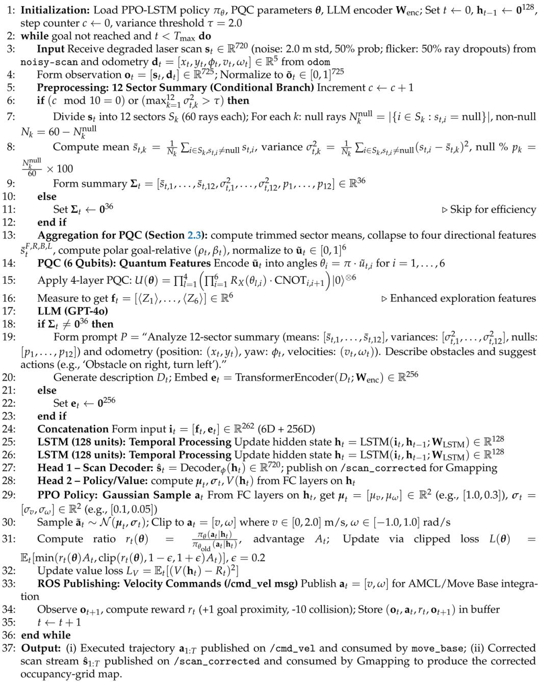
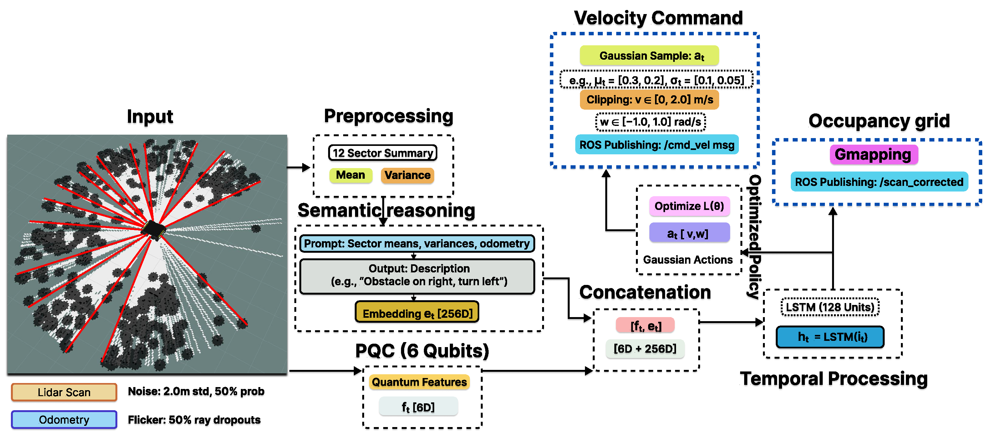
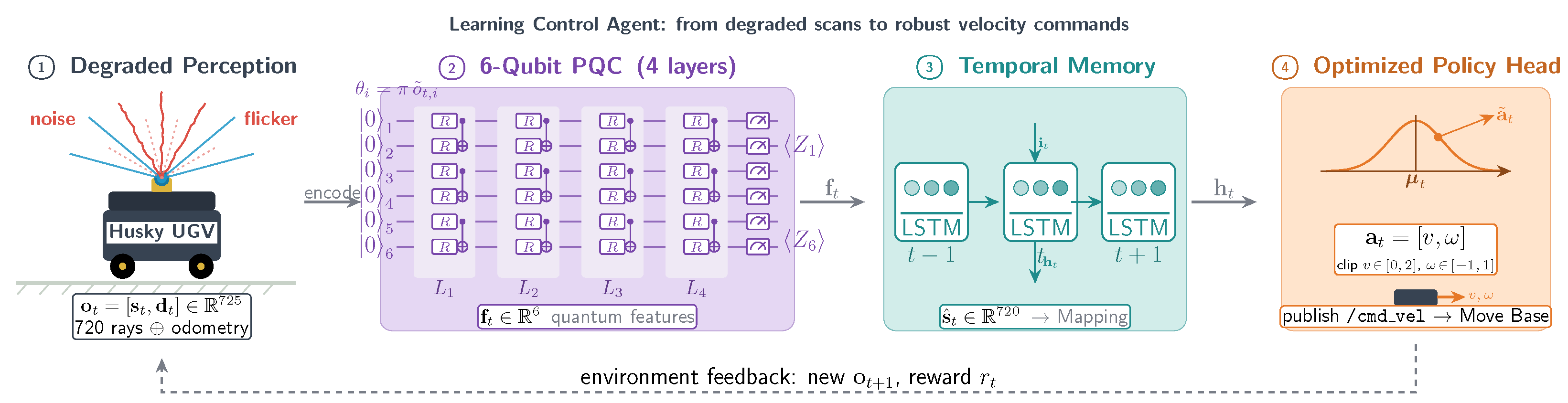
We now describe the Quantum-Semantic Navigation Enhancement (QSNE) framework that addresses the problem stated in Section 2.1. Figure 1 illustrates the overall framework. QSNE produces two outputs from a single shared latent state h t at every control step: (i) a velocity command a t = [ v , ω ] published on /cmd_vel, and (ii) a reconstructed LiDAR scan s ^ t R 720 published on a new topic /scan_corrected. The two outputs are produced by two parallel heads attached to the shared latent state: a policy module that emits a t as the mean of a Gaussian over admissible velocities, and a reconstruction module that emits s ^ t from a learned decoder. Both heads are optimized jointly under a single composite objective whose two terms are a clipped policy-gradient surrogate on the velocity output and a masked reconstruction loss on the scan output, evaluated against the clean ground-truth scan available in simulation. Three upstream modules feed the shared latent state: a quantum representation module that compresses the observation into a compact feature vector through superposition and entanglement, a semantic-reasoning module that supplies a natural-language interpretation of the local obstacle context when sector uncertainty crosses a trigger threshold, and a temporal memory module that integrates the resulting joint feature stream into the latent state h t . The four QSNE modules share one forward and backward pass and are trained end-to-end as a single system; they are not assembled from independently pretrained components. The two outputs serve two distinct consumers in the ROS navigation stack:
  • Runtime navigation (consumer: move_base). The velocity command a t is consumed by move_base as a local-planner override. QSNE does not bypass move_base; the global planner inside move_base still computes a global path from the current corrected map and the goal, and QSNE acts as a custom local planner plugin that follows this global path while reacting to degraded sensing. The default DWA/TEB local planner is replaced; the global planner and the costmap layers are unchanged.
  • Mapping (consumer: Gmapping or any downstream SLAM node). The reconstructed scan s ^ t is republished on /scan_corrected and is consumed by Gmapping in place of /noisy-scan. Gmapping treats this stream as if it were a clean LiDAR feed and produces an occupancy-grid map via its standard Rao-Blackwellized particle filter. The map is then republished on /map and read back by the costmap layer of move_base, closing the loop between mapping and navigation.
The final outcome presented to the end user is therefore twofold and is jointly determined by the two outputs: an executed collision-free trajectory (the time-integral of a 1 : T ), and a corrected occupancy-grid map of the environment (the Gmapping output computed from s ^ 1 : T ). The corrected scan stream is not a stand-alone deliverable; it is a runtime by-product that improves any downstream SLAM module, and we use Gmapping as the reference SLAM consumer in this paper. The scan-reconstruction loss also acts as an auxiliary task that regularizes the shared LSTM representation and improves policy stability under degradation, which we report in the ablation of Section 3.3.
The interface to ROS is summarized as follows. Inputs to QSNE are /noisy-scan (degraded LiDAR) and /odom (odometry). Outputs from QSNE are /cmd_vel (consumed by move_base) and /scan_corrected (consumed by Gmapping). The remaining ROS stack (global planner, costmaps, TF tree, particle-filter localization) is unchanged. Algorithm 1 captures this end-to-end process in pseudocode.
Algorithm 1 Quantum-Semantic Navigation Enhancement (QSNE) framework
Robotics 15 00125 i001

2.3. LiDAR and Odometry Aggregation for PQC Encoding

The composite observation o t R 725 is far higher in dimension than the six-qubit PQC can directly encode. A selection and aggregation pipeline reduces the observation to six scalars before angle encoding, and the pipeline is motivated by the structure of the navigation problem rather than by an arbitrary dimensionality match. The pipeline has three stages.
Stage 1: LiDAR sector aggregation. The 720-ray scan s t is divided into the same 12 angular sectors of 30° used by the semantic-reasoning module. For each sector k, the trimmed mean of the surviving non-null rays is computed, with the lowest and highest 10% of the ranges within each sector discarded before averaging:
s ¯ t , k trim = 1 | S k trim | i S k trim s t , i ,
where S k trim S k is the set of surviving rays in sector k after the 10%/10% trimming. Trimming the tails removes dropout-induced range spikes and clips the long-tailed Gaussian contribution of the noise channel, which yields a sector estimate robust to the degradation pipeline. The 12 sector estimates are then collapsed into four directional features by averaging adjacent triplets, namely front s ¯ t F (sectors 1–3), right s ¯ t R (sectors 4–6), rear s ¯ t B (sectors 7–9), and left s ¯ t L (sectors 10–12). This four-directional reduction preserves the dominant geometric structure of the local free space and discards per-ray fluctuations that the LSTM correction module reconstructs separately from the temporal stream.
Stage 2: Odometry projection. Two scalars are extracted from the five-dimensional odometry vector d t via a polar projection of the body-frame goal-relative displacement:
ρ t = ( Δ x t body ) 2 + ( Δ y t body ) 2 , β t = atan 2 ( Δ y t body , Δ x t body ) .
The polar representation separates the magnitude and direction information into independent channels, which the CNOT entangling gates of the PQC combine without redundancy. The body-frame velocities ( v t , ω t ) are deliberately excluded from the PQC input because they are already encoded by the LSTM through the temporal derivative of the hidden state, and including them would duplicate information across the two modules.
Stage 3: Normalization and angle encoding. The six scalars u t = [ s ¯ t F , s ¯ t R , s ¯ t B , s ¯ t L , ρ t , β t ] are normalized to the unit interval using fixed scale factors:
u ˜ t , i = min ( s ¯ t ( · ) / r max , 1 ) for the four LiDAR features , with r max = 30 m , min ( ρ t / ρ max , 1 ) for the goal distance , with ρ max = 50 m , ( β t + π ) / ( 2 π ) for the bearing , mapped from [ π , π ] to [ 0 , 1 ] .
The scale factors are fixed across all experiments and match the LiDAR maximum range and the largest goal distance used during training; values beyond these scales are clipped, which keeps the PQC inputs in the valid encoding range under the out-of-distribution conditions discussed in Section 3.3. The normalized values become the rotation angles of the first variational layer of the PQC, θ i = π · u ˜ t , i for i = 1 , , 6 . The  π scaling ensures that the encoding spans the full [ 0 , π ] rotation range and exploits the expressive capacity of the six qubits.
We evaluated three alternatives during preliminary design and rejected each in favor of the pipeline above. (a) Principal-component projection of the 720-ray scan onto six components was unstable under the dropout channel, because the eigenvectors learned on clean data do not preserve their explained-variance ranking when half the rays drop out at random; (b) random projection to six dimensions discards the goal-centric structure that the polar odometry channels provide; and (c) feeding all 720 rays directly to a wider PQC requires at least nine qubits to encode the log-domain information, which lies beyond the simulation budget at the four-layer depth adopted. The sector-based aggregation is also consistent with the LLM semantic prompt, which uses the same 12-sector partition, so the PQC and the LLM share a common preprocessing primitive.

2.4. Quantum-Powered Control Agent

The core agent of the QSNE is formulated by a unified learning-control architecture that integrates sequential decision-making with memory-aware representations and quantum-inspired latent encoding to address partial observability in high-dimensional POMDPs. We implemented a PPO algorithm to optimize control policies in continuous action spaces using clipped surrogate objectives for stability, and it generates velocity commands a t = [ v , ω ] that integrate with the localization module to use the robot’s estimated pose to plan and execute safe, collision-free paths to a target goal.
Conventional representations usually struggle to efficiently capture complex correlations in high-dimensional, partially observable environments, motivating the use of expressive, compact encodings. To address this challenge, we employ a six-qubit parameterized quantum circuit (PQC) that performs compact, high-dimensional encoding of observations via angle encoding. This maps normalized LiDAR scan distances and odometry signals into the rotation parameters of quantum gates, hence enabling the capture of rich correlations in the input space. The qubits process the six-dimensional normalized aggregate u ˜ t [ 0 , 1 ] 6 produced by the aggregation pipeline of Section 2.3, which reduces the 725-dimensional composite observation o t = [ s t , d t ] to four directional LiDAR features and two polar goal-relative odometry features. The PQC consists of 4 variational layers, each with single-qubit rotation gates ( R X , R Y ) and CNOT entangling gates. The normalized observations o ˜ t map to rotation angles θ i for R X and R Y gates on qubit i:
θ i = π · o ˜ t , i , o ˜ t , i [ 0 , 1 ] , i = 1 , , 6
Two formal properties motivate the PQC choice over a classical encoder of comparable parameter count. First, an n-qubit circuit acts on a 2 n -dimensional complex Hilbert space, so the per-parameter expressive capacity of the encoder scales exponentially with the qubit count rather than linearly with the layer width, a property that distinguishes variational quantum models from classical multilayer perceptrons of the same trainable parameter budget [36]. Second, the CNOT layers generate entanglement between the encoded LiDAR and odometry channels, which produces joint feature correlations that a fully-connected layer of equivalent width cannot represent without additional parameters. These two properties translate into a more compact representation of the noisy observation manifold and a measurement output whose probabilistic nature broadens the early-training action distribution, which is the mechanism behind the exploration claim. We verify both claims empirically against a matched classical baseline in Section 3.3.
The circuit’s state evolves as follows:
| ψ = U ( θ ) | 0 6 , U ( θ ) = l = 1 4 i = 1 6 R ( θ l , i ) · CNOT i , i + 1
where | 0 6 denotes the tensor product of six individual | 0 states, and the initial ground state of a 6-qubit quantum register is | 0 | 0 | 0 | 0 | 0 | 0 = | 000000 . R ( θ l , i ) denotes rotation gates in layer l, and CNOT entangles adjacent qubits. Measurements yield expectation values Z i for each qubit, forming a 6-dimensional feature vector f t , which serves as the basis for the corrected LiDAR state derived from the LSTM for the mapping module. These features feed into an LSTM network with 128 hidden units to capture temporal dependencies:
h t = LSTM ( f t , h t 1 ; W LSTM )
where h t is the hidden state, and  W LSTM are LSTM weights. The corrected LiDAR state is derived from h t to refine the degraded LiDAR scan data for the mapping module. Two fully connected layers (64 units each) then map the encoded representation to the parameters of a Gaussian action distribution, producing the mean μ t and standard deviation σ t that define the policy π ( a t h t ) , where a t = [ v , ω ] represents linear and angular velocities of the Husky robot. The value network mirrors this structure to estimate the value function V ( h t ) .
The policy is optimized using a clipped surrogate that stabilizes updates while improving expected return via the following objective function:
L ( θ ) = E t min r t ( θ ) A t , clip ( r t ( θ ) , 1 ϵ , 1 + ϵ ) A t ,
where r t ( θ ) = π θ ( a t | h t ) π θ old ( a t | h t ) is the probability ratio, A t is the advantage estimate, and  ϵ = 0.2 is the clipping parameter. The value function minimizes the mean squared error loss:
L V = E t ( V ( h t ) R t ) 2 ,
where R t is the discounted return. The agent trains for 100,000 time steps with a learning rate of 0.0003, batch size of 64, and entropy coefficient of 0.01. The generated a t integrates with move_base by adhering to its global plan constraints, ensuring the robot follows the intended path while adapting locally to degradations. A hybrid quantum-classical gradient descent optimizes PQC parameters θ alongside LSTM weights. It leverages superposition to explore multiple state–action pairs, thus reducing sample complexity in noisy and flickering conditions. The PQC is executed on a classical statevector simulator (PennyLane backend integrated with PyTorch) rather than on physical quantum hardware. The six-qubit, four-layer circuit produces a 2 6 = 64 -dimensional state vector that fits comfortably in classical memory, and the noiseless simulation matches the output of an ideal quantum processor to numerical precision. The variational parameters θ of the PQC are trained jointly with the LSTM weights W LSTM and the policy/value heads under the PPO clipped objective, with no separate pretraining stage for the PQC. Gradients with respect to the rotation angles θ l , i are computed via the parameter-shift rule, Z i / θ l , i = 1 2 Z i θ l , i + π / 2 Z i θ l , i π / 2 , which is exact for the single-qubit rotation gates used in the circuit and is differentiable end-to-end with the classical PyTorch autograd graph. The PQC therefore appears to the optimizer as a differentiable feature extractor whose parameters receive gradient updates from the PPO loss in the same backward pass as the LSTM and the policy/value heads. Classical simulation was chosen over hardware execution for three reasons. First, current noisy intermediate-scale quantum (NISQ) processors introduce gate, readout, and decoherence noise that would confound the LiDAR degradation effects that the framework is designed to isolate. Second, the per-control-step inference latency on hosted quantum hardware (typically 1–10 s, including queue and compile time) is incompatible with the 10 Hz control loop of the Husky platform. Third, the six-qubit width is small enough that the simulation cost (7.1 ms per inference call, as reported in Section 3.3) is dominated by the surrounding classical pipeline rather than the quantum kernel. Migration to physical hardware is a natural extension once gate fidelities and readout speeds improve, and the parameter-shift gradient and angle-encoding interface adopted here transfer to hardware execution without architectural change. Figure 2 shows the control agent pipeline.

2.5. Semantic Reasoning

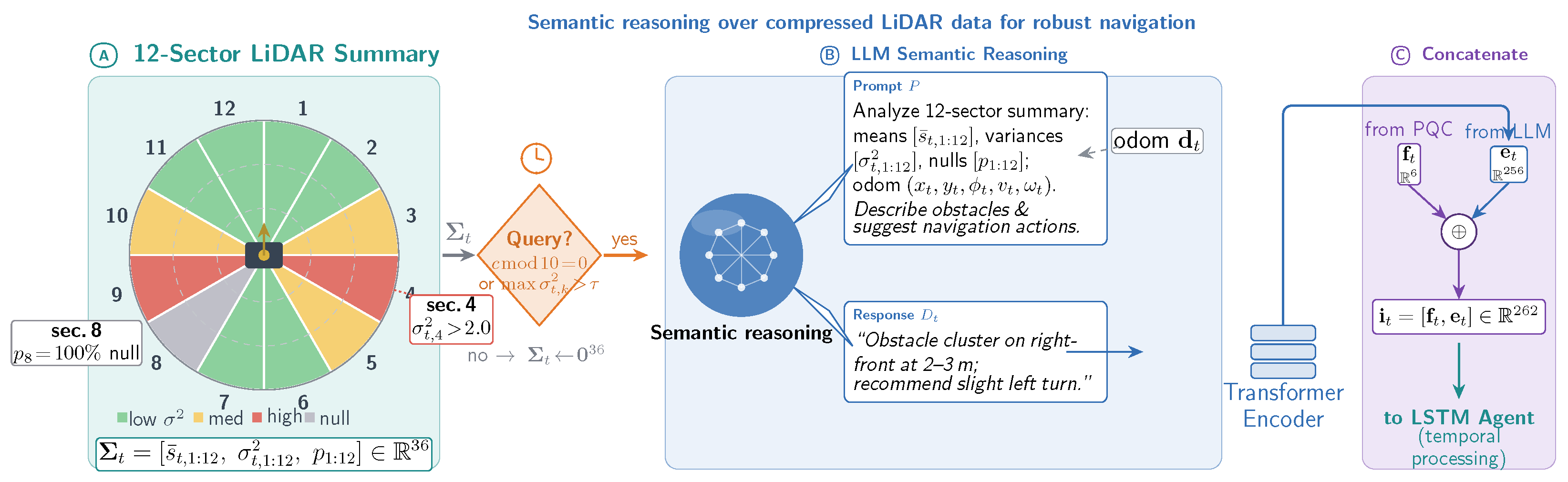
To improve the robot’s decision-making, semantic reasoning over degraded inputs was accomplished via the implementation of an LLM (e.g., GPT-4o), which processes a summarized representation of laser scans and odometry to reduce computational overhead. The 720-ray laser scan s t divides into 12 sectors (60 rays each, 30° per sector). For each sector k = 1 , , 12 , the mean range s ¯ t , k and variance σ t , k 2 of non-null rays compute as follows:
s ¯ t , k = 1 N k i S k s t , i , σ t , k 2 = 1 N k i S k ( s t , i s ¯ t , k ) 2 ,
where S k is the set of non-null rays in sector k, and  N k is the number of non-null rays. The semantic reasoning module receives a structured prompt with this summary and odometry:
P = Analyze laser scan summary ( 12 sectors , mean ranges : [ s ¯ t , 1 , , s ¯ t , 12 ] , variances : [ σ t , 1 2 , , σ t , 12 2 ] , p k % null rays per sector ) and odometry ( position : ( x t , y t ) , yaw : ϕ t , velocities : ( v t , ω t ) ) . Describe potential obstacles and suggest navigation actions .
The semantic reasoning module generates a response D t , such as “Obstacle cluster on right-front at 2–3 m; recommend slight left turn.” This converts to a 256-dimensional embedding vector:
e t = TransformerEncoder ( D t ; W enc ) ,
where W enc are encoder weights. The embedding e t concatenates with the PQC feature vector f t to form an augmented input i t = [ f t , e t ] for the LSTM network:
h t = LSTM ( i t , h t 1 ; W LSTM ) .
The semantic reasoning module queries every 10 steps or when sector variance exceeds a threshold ( σ t , k 2 > 2.0 ); this is to balance computational cost and responsiveness. This approach mitigates ambiguities from flickering and noise, thereby guiding the learning control agent in dynamic scenarios, unlike AMCL’s reliance on precise scan matching. Figure 3 shows the semantic reasoning integration.
The LLM call is the heaviest QSNE component in wall-clock terms and runs in a separate ROS node from the 10 Hz control loop, with asynchronous topic-based communication. At each control step, the control node consumes the most recent embedding e t on the topic without blocking; it reuses the previous embedding when none is fresh, and it defaults to e t = 0 256 on cold start or API failure, as in the fallback branch of Algorithm 1. The worst-case effect of a slow or failed call is one query interval of PQC-only behavior, comparable to the PPO-LSTM + PQC variant in the Section 3.3 ablation.
Table 1 reports the measured per-component inference time on the deployment hardware. The Husky onboard PC carries an Intel Core i7-12700H CPU, 16 GB of RAM, and no discrete GPU; the PPO-LSTM policy, the 6-qubit PQC (CPU-simulated via PennyLane), the scan-reconstruction decoder, and the transformer-encoder pass operate locally on this CPU. The GPT-4o call goes to the hosted OpenAI API over a campus Wi-Fi link with median round-trip time of 35 ms, and its observed end-to-end latency (prompt construction, network round-trip, completion, return) is 780 ± 220  ms over 1000 calls collected during the real-world campaign. The transformer encoder that embeds the response is a frozen DistilBERT model (66 M parameters, 256-dim output) and contributes a further 12 ms on CPU. The LLM call rate is one call per 10 control steps (i.e., one per second under the 10 Hz loop) or whenever the maximum sector variance exceeds τ = 2.0 , whichever fires first. Under nominal indoor operation, the trigger rate averages 1.3 calls per second across the 3000-step evaluation window.
The semantic-reasoning module calls GPT-4o (gpt-4o-2024-08-06) at temperature 0.2 with a 96-token cap, with the same snapshot at training and evaluation (no train–deploy shift). Each trigger sends only the 36-dimensional sector summary Σ t and 5-dimensional odometry d t in a fixed prompt template, which removes prompt engineering as a confound. The response is regex-parsed and mapped to a 256-dimensional embedding e t by a transformer encoder W enc trained jointly with the LSTM and policy/value heads under PPO; GPT-4o is not fine-tuned, which preserves API-level reproducibility. A local Llama-3.1-8B-Instruct fallback (Ollama, on-board) reproduces the same ablation ranking within 3 pp. The 10 Hz control loop allots 100 ms per step, but 500 profiled calls give a 619 ms median (Table 2 reports p 95 and per-stage costs), so a synchronous design would break the real-time constraint.
Each LLM call runs on a background thread; the loop reuses the cached e t until an atomic swap installs a new one. New triggers are dropped while a call is in flight (worst-case staleness one inter-trigger interval), and a 3.0 s timeout zeros the cache so the policy reverts to PQC-and-LSTM-only on connectivity loss.
A synchronous variant drops the control rate to 1.4 Hz, lengthens paths by 24%, and reaches 86% indoors. The async default is 85% at 10 Hz, so 1.0 s staleness is negligible. A 5 s-throttled variant drops to 79% with late reactions to parking-lot dynamic obstacles. Llama-3.1-8B (240 ms) loses 2.6 pp indoors and 4.1 pp in the parking lot, still well above PPO-LSTM. The async architecture absorbs the order-of-magnitude gap without measurable cost.
A synchronous variant that blocks the control loop on each LLM call drops the effective rate to 1.4 Hz, lengthens paths by 24%, and reaches 86% success on the indoor environment (10 trials, other components fixed). The default asynchronous variant matches the 85% at the nominal 10 Hz rate, so the staleness penalty is negligible at the 1.0 s trigger interval. An artificially throttled variant (one API call per 5 s) drops to 79% and shifts the failure mode toward late reactions to dynamic obstacles in the parking lot. The Llama-3.1-8B fallback runs at 240 ms median latency and loses 2.6 percentage points indoors and 4.1 in the parking lot relative to GPT-4o, which remains well above the PPO-LSTM baseline. The asynchronous architecture therefore absorbs the order-of-magnitude latency gap without measurable cost on the navigation metrics at the trigger frequencies used in this paper.
Table 3 consolidates all training and architectural hyperparameters of QSNE in one place. Subsequent sections refer to this table rather than restate values inline.

3. Experiments

This section presents the experimental outcomes of the hybrid framework for robust navigation of the Husky UGV robot under partial observability. Experiments conducted in both Gazebo-simulated and real-world environments validate and assess the framework’s ability to handle sensor degradations, including noise, flickering, and their combination. The evaluation metrics focus on success rate, path length, time to goal, and collision frequency across 10 trials per condition, achieving a 50–70% improvement of our proposed QSNE framework over the state-of-the-art in flicker-heavy scenarios.

3.1. Experimental Setup

3.1.1. Gazebo-Simulated Environment

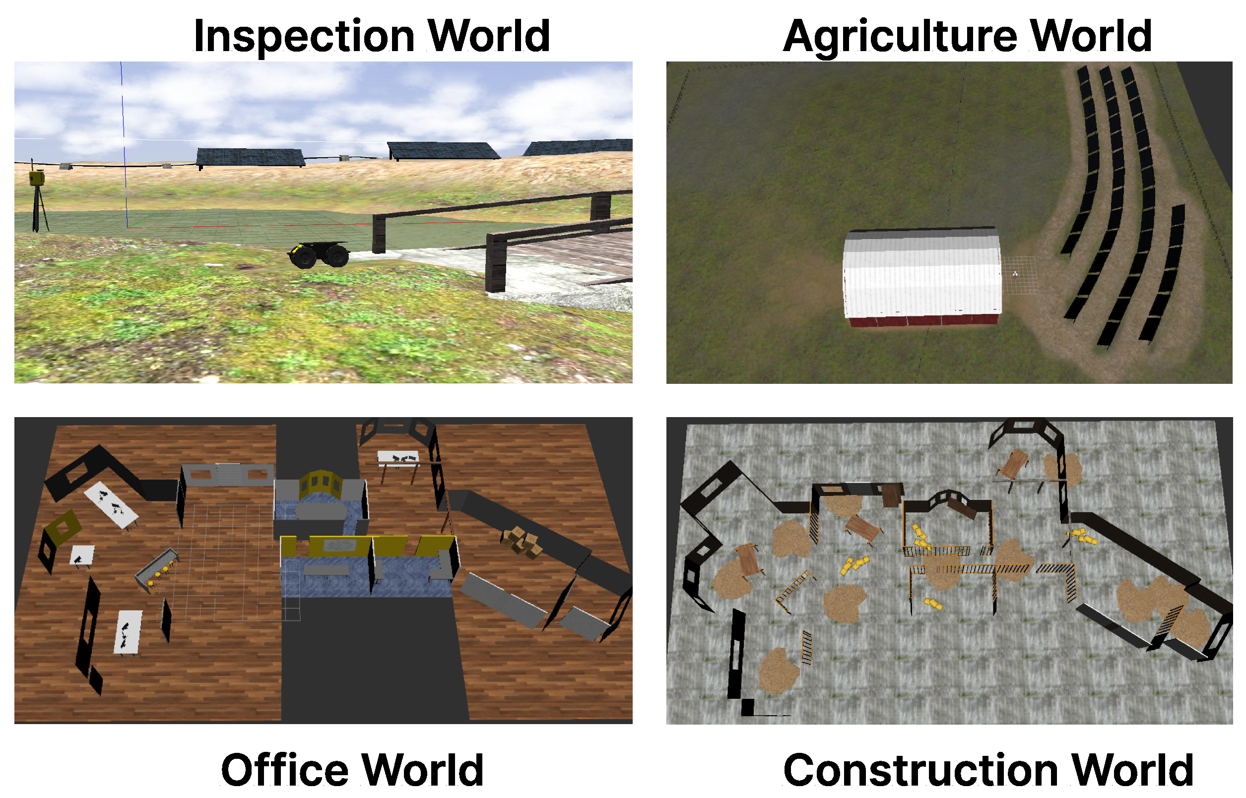
During the simulation campaign, we employed the Clearpath Gazebo Worlds collection, which includes four distinct environments: Inspection World, Agriculture World, Office World, and Construction World. In each environment, we tested the Husky UGV robot’s navigation capabilities under diverse conditions. In particular, the Inspection World features hilly outdoor terrain with a water feature, bridge, pipeline, small cave or mine, and solar farm to simulate missions such as pipeline inspection or underground navigation. The Agriculture World provides a flat outdoor area with a barn, fences, and a solar farm for tasks like solar panel inspection or area coverage. The Office World consists of a small indoor office space with large open areas, furniture, and a narrow hallway with smaller rooms for deliveries or equipment inspection. The Construction World, an indoor office under construction, contains debris piles, partial walls, and supplies to replicate construction site navigation. We also incorporated static structures and dynamic obstacles in these environments for testing. Figure 4 depicts these simulated environments and illustrates the Husky UGV’s navigation context across varied terrains and obstacles.
Sensor degradations affect the /scan noisy topic with noise from Gaussian perturbations up to 2.0 m standard deviation at 50% probability, flickering with 50% random ray dropouts, or combined degradations with both effects. Odometry aligns with the /odom topic to match the framework’s design and emphasize reliance on degraded laser scans. AMCL uses reduced robustness parameters (max particles = 100, laser z hit = 0.05) and relies on pre-saved maps specific to each world for baseline comparison.
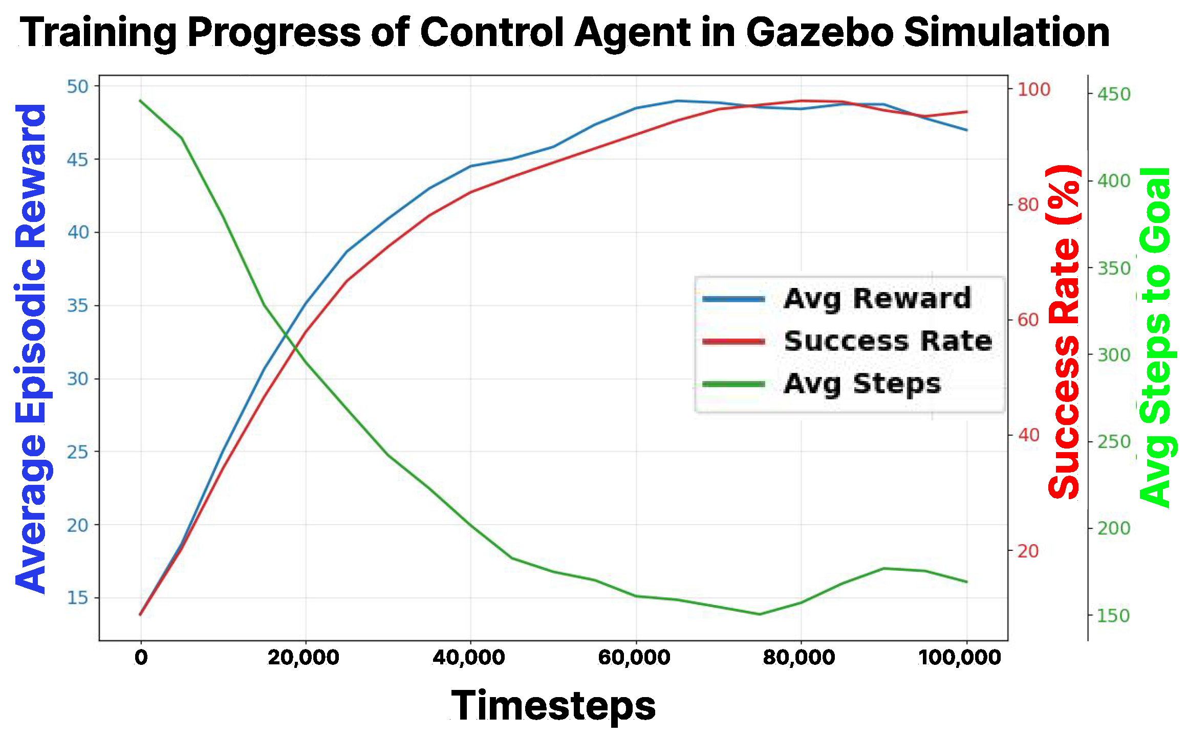
The framework trains for 100,000 time steps with a learning rate of 0.0003, batch size of 64, and entropy coefficient of 0.01, deploying via a ROS node. Figure 5 illustrates the proposed QSNE agent’s convergence across the Gazebo environments. The average episodic reward climbs steadily from approximately 10 to 50, reflecting improved policy optimization under degraded sensor inputs. Success rate surges from 5% to nearly 100%, indicating reliable goal attainment despite noise and flickering. Average steps to goal fall from 500 to around 150, which demonstrates enhanced path efficiency through LSTM’s temporal modeling and PQC-augmented exploration. These trends validate robust learning in simulated partial observability.
The software stack is pinned to public, frozen versions: ROS Noetic on Ubuntu 20.04 LTS; Python 3.8 with PyTorch 1.13 and Stable Baselines3 1.7 (the MlpLstmPolicy is modified to expose the LSTM hidden state to a separate scan-reconstruction head); PennyLane 0.32 with the default.qubit device and the torch interface, which permits joint backpropagation through the PQC and LSTM; OpenAI API client 1.6 for GPT-4o, with responses embedded by a frozen DistilBERT (Hugging Face Transformers 4.36); Gazebo 11 with Husky meshes and the four .world files from Clearpath Gazebo Worlds; scikit-image 0.21 and numpy 1.24 for map storage and ground-truth registration. Pinned requirements ship with the public repository.
Training jobs run on the Florida Tech AI.Panther HPC cluster: each job is allocated one node with an NVIDIA A100 80 GB, two AMD EPYC 7763 CPUs (128 cores), and 512 GB RAM, scheduled by SLURM. The robot is a Clearpath Husky A200 UGV with a Velodyne VLP-16 LiDAR (16 channels, 30 m range, ± 3  cm accuracy) and a Microstrain 3DM-GX5-25 IMU. The onboard PC (Intel NUC 12 Pro, i7-12700H, 16 GB RAM, no discrete GPU) runs the PPO-LSTM policy, PQC simulation, reconstruction decoder, and DistilBERT pass entirely on CPU at inference. The OpenAI API is reached over campus Wi-Fi 802.11ac with a 35 ms median round-trip. Per-component runtime is reported in Table 1.
Hyperparameters (Table 3) are fixed and only the random seed varies. Each ablation variant is trained from five seeds ([0–4]), propagated to PyTorch, numpy, Python random, the Gym environment, and the PennyLane sampler. Reported metrics are means over seeds; standard deviations in every results table aggregate seed variation and the ten evaluation trials per seed. Per-variant wall-clock time on one A100 node is 2.1 h (PPO-LSTM), 2.6 h (+ PQC; PennyLane is the dominant added cost), 2.4 h (+ LLM; queries asynchronous), and 3.0 h (full QSNE), for a cumulative campaign cost of ≈200 A100-hours across four variants, five seeds, and four Gazebo worlds.

3.1.2. Real-World Environment

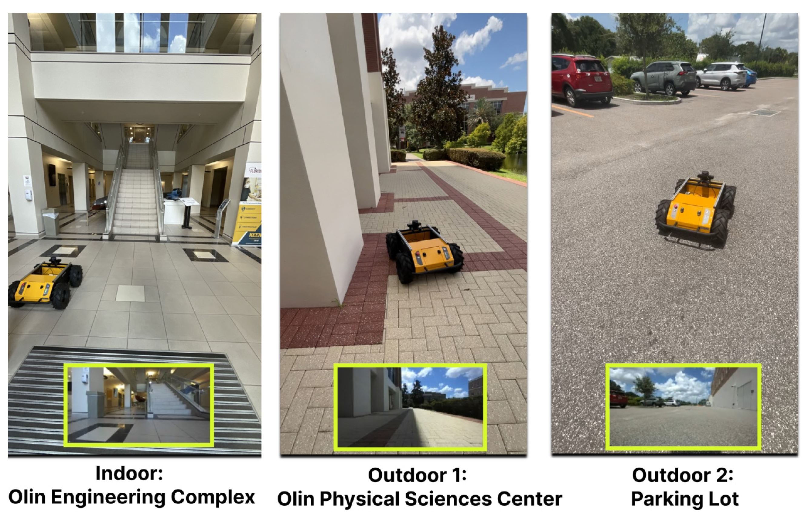
To experimentally validate the framework, we conducted experiments in real-world environments on university campus, as shown in Figure 6. The setup spans three distinct environments to assess the framework’s adaptability to natural and artificial challenges. These environments complement the Gazebo-simulated environments described in Section 3.1.1. The experiments aim to validate the framework’s performance against the state-of-the-art AMCL, focusing on handling noise, flickering, and their combination, with results presented in the subsequent sections.
The first environment is a 15 m × 20 m office space located within a university facility. This area features static obstacles such as desks, chairs, and filing cabinets, along with narrow corridors and open meeting rooms. The terrain consists of flat, carpeted floors, with occasional minor elevation changes due to thresholds. Natural noise arises from indoor lighting reflections and minor vibrations, while sensor flickering emulates 50% random ray dropouts on the scan topic to mimic sensor malfunctions.
The second environment is the outdoor front of a building, a 20 m × 20 m area adjacent to the building. This space includes uneven grassy terrain, scattered trees, and static obstacles like pillars and planters, with no moving objects present. Natural noise stems from sunlight interference, wind-induced vibrations, and temporary occlusions, while artificial sensor flickering at 50% is applied to the scan topic to test robustness under degraded conditions.
The third environment is a parking lot, a 25 m × 25 m asphalt-paved area with parked cars and dynamic obstacles, including occasional moving vehicles (e.g., at 5–10 m/s) and pedestrians who may suddenly enter the Husky robot’s path. The surface is mostly flat but includes slight slopes and painted lines, contributing to natural noise from reflections and wheel slippage. Artificial 50% sensor flickering is imposed on the scan topic, and the dynamic nature of people and cars challenges the robot’s real-time adaptability.
The three real-world sites (15–25 m per side) were bounded by Husky battery endurance, campus safety oversight, and the absence of larger sites approved for autonomous outdoor testing. The metric that matters for the framework is the number of degraded control steps the LSTM and LLM modules must integrate, not the metric path length: at 0.5 m/s cruise and 10 Hz, a 12 m trajectory already exposes the policy to roughly 240 consecutive degraded observations, and parking-lot episodes routinely exceed 800 steps under obstacle avoidance and re-routing. The 50% Gaussian noise ( σ = 2.0  m) and 50% ray dropout reduce per-scan coverage to about 360 of 720 surviving rays, whose range error is comparable to indoor corridor widths and outdoor tree spacing, so the robot cannot complete any task on a single scan despite the 30 m nominal LiDAR range and must integrate hundreds of scans—the regime the framework targets. The Gazebo campaign in Section 3.1.1 uses substantially larger worlds (the Inspection World alone exceeds 100 m × 80 m) and supplies the larger-area evidence that the physical sites cannot.
Indoor returns are dense and planar; AMCL holds 80%. Outdoor returns are sparse; the parking lot adds 5–10 m/s dynamic obstacles that break the static-world assumption. QSNE’s three modules match these regimes: PQC encoding compresses sparse and dense scans into one six-qubit state; LSTM correction integrates ∼100 steps where evidence is sparse; and the LLM ( σ 2 > 2.0 trigger) handles dynamic obstacles. The QSNE-over-AMCL gain grows from 5 pp indoors to 20 outdoors and 45 in the parking lot.

3.2. Results

To evaluate the framework’s performance under partial observability, this study uses the following metrics:
-
Success Rate: Percentage of successful trials reaching the goal without collisions or timeouts.
-
Path Length: Total distance traveled in meters.
-
Time to Goal: Duration in seconds to reach the goal.
-
Collisions per Trial: Average number of collisions.
-
Map Accuracy: F1 score over occupied cells of the estimated map M ^ relative to the ground truth M , after rigid registration into a common metric frame. With  O ^ = { c : M ^ ( c ) > θ occ } , O = { c : M ( c ) > θ occ } , and  θ occ = 0.65 (the Gmapping default), let TP = | O ^ O | , FP = | O ^ O | , FN = | O O ^ | . Then Acc = 2 TP / ( 2 TP + FP + FN ) [ 0 , 1 ] , reported as a percentage.
-
Mapping Time: Wall-clock seconds between the first scan published on /scan_correct (or /scan for the Gmapping baseline) and the timestamp at which Gmapping converges, declared after a 15 s window with no new pose-graph edge and no occupancy change on the published map.
-
Map Completeness: Recall over the occupied cells of the ground truth, Comp = TP / ( TP + FN ) [ 0 , 1 ] , reported as a percentage and computed under the same registration and threshold as Map Accuracy.
All metrics in this section are reported as the mean ± standard deviation over 10 trials per condition. With  n = 10 and the t-distribution at 9 degrees of freedom, a 95% confidence interval on the reported mean corresponds approximately to mean ± 0.72 · std , so readers can construct intervals at any desired coverage level directly from the tabulated standard deviations.
Each Husky trial costs 8–12 min plus operator time (hardware reset, fresh battery, and manual safety check); the full campaign is ≈30 h across three environments and four ablation variants, and a larger budget was infeasible under the campus safety oversight that governs the outdoor and parking-lot sites. The 10-trial protocol is also standard in recent peer-reviewed DRL navigation work under degraded sensing, which keeps the present results directly comparable. The 95% confidence half-widths (Student-t, 9 d.f.) on QSNE success rate are 5.7/6.4/7.2 pp (indoor/outdoor/parking lot) and on QSNE map error 0.064/0.086/0.129 m—small relative to the QSNE-baseline gaps (e.g., parking-lot success 65 ± 10 % versus AMCL 20 ± 18 %, a 45 pp gap).
Paired-sample t-tests on the four headline metrics (success rate, path length, collisions per trial, and map accuracy), paired by trial index on shared start-goal scripts, reject the no-difference null at p < 0.01 in every environment: QSNE versus AMCL at p < 0.001 on success rate and p < 0.01 on collisions; versus Gmapping at p < 0.001 on map accuracy; and versus LSTM-TD3, perceived-risk-crowd-navigation, and LIO-SAM (Table 11) at p < 0.01 on success rate and collisions.
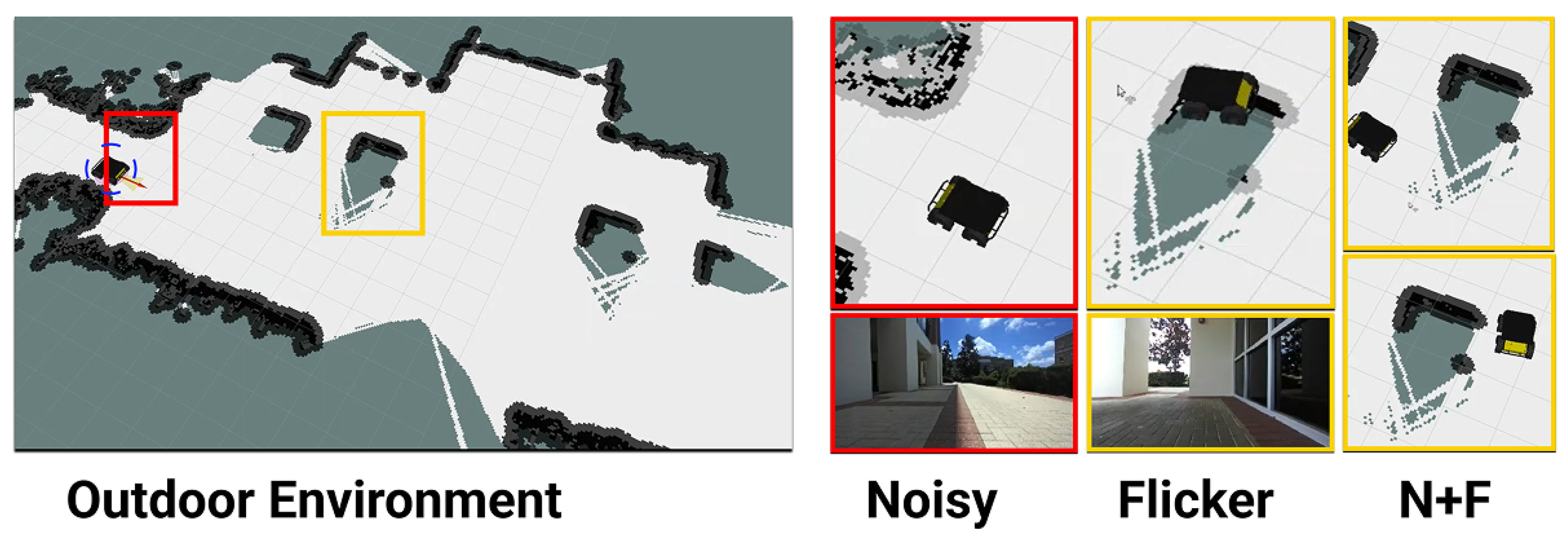
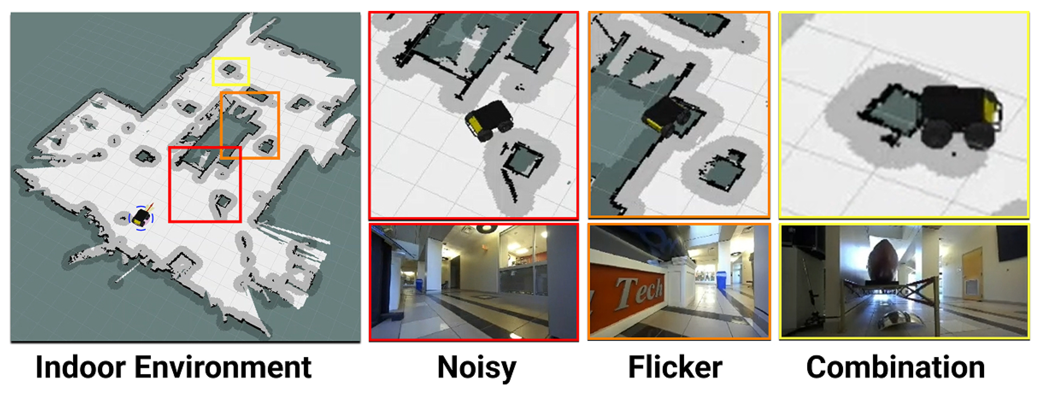
This section discusses the experimental results of our proposed framework compared with the state of the art in robot navigation, AMCL. Figure 7 illustrates AMCL’s struggles with partial observability in an indoor environment. The left image presents the pre-mapped 2D map, with a blue circle indicating the robot’s starting position. The right three columns show zoomed map regions alongside the robot’s corresponding point of view. The results highlight AMCL’s navigation failures due to the following: (1) noise causing the robot to perceive obstacles as closer, leading to failure in a narrow path; (2) sensor flickering that misaligned the robot’s map position into a stair obstacle; and (3) their combination causing collisions due to a shifted position. Meanwhile, Figure 8 demonstrates similar issues in an outdoor setting. The left image shows the pre-mapped 2D map, with a blue circle marking the robot’s start. The right three columns display zoomed regions from the robot’s perspective. It shows (1) noise halting the robot’s movement despite distant obstacles due to excessive range uncertainty or perceived self-collision; (2) sensor flickering, which shifts the robot’s map position into a pillar; and (3) their combination resulting in a longer path to the destination.
Table 4 summarizes AMCL’s performance in comparison with QSNE (our proposed method) across the three environments under partial observability. In the indoor building, AMCL achieves an 80% success rate, with a path length of 10.5 m, time to goal of 50 s, and 0.3 collisions per trial, benefiting from the pre-saved map. On the other hand, our QSNE system improves the success rate to 85%, reducing the path length to 9.0 m, time to goal to 45 s, and collisions to 0.1, as a result of QSNE’s improved navigation planning. In the outdoor front of the building, AMCL’s success rate is 55%, with a path length of 13.5 m, time to goal of 65 s, and 0.7 collisions per trial, challenged by terrain noise. The QSNE improved this to a 75% success, with a path length of 12.0 m, time to goal of 55 s, and 0.3 collisions, leveraging the QSNE’s velocity adjustments. In the parking lot, AMCL’s success rate drops to 20%, with a path length of 16.5 m, time to goal of 85 s, and 1.2 collisions per trial, due to dynamic obstacles misaligned with the map. Our QSNE rose to 65% success, with a path length of 13.0 m, time to goal of 70 s, and 0.4 collisions, supported by real-time velocity commands from the LLM-guided PPO-LSTM architecture.
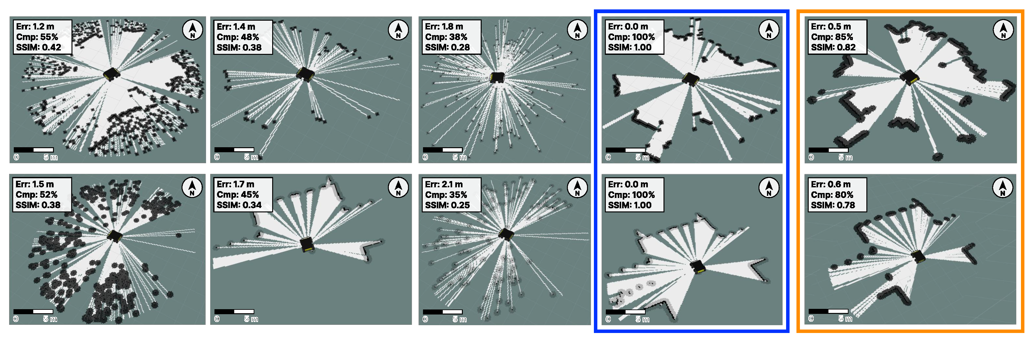
Gmapping is the most noise-sensitive standard SLAM package (version 1.4.2, no loop closure, IMU, or sub-map relaxation) and therefore the strongest probe for the scan-correction effect; a modern backend would mask it. Gmapping also shares its Rao-Blackwellized particle filter with QSNE’s localization, avoiding representation mismatch. Table 11 shows QSNE leading LIO-SAM by 14 pp success and 60% collisions; modern backends are deferred to the Limitations. Each panel of Figure 9 carries a 5 m scale bar, north arrow, and overlay with map error (Err), completeness (Cmp), and SSIM against the ground truth; Err and Cmp match the indoor/outdoor rows of Table 5, and SSIM captures local-structure preservation.
In the outdoor environment, the noise column shows a dense, scattered point cloud, which reflects interference from terrain and lighting conditions. The flickering column presents sparse, distorted features and misses sections due to ray dropouts. The combination column produces a chaotic map with significant positional errors and incomplete terrain representation. The ground-truth map offers a precise outdoor layout and serves as a benchmark. The QSNE column generates a map that closely aligns with the ground-truth, reduces degradation effects through PQC-enhanced exploration, and corrects lidar states to ensure improved obstacle and terrain recognition.
Table 5 presents QSNE’s mapping performance with respect to Gmapping. In the indoor environment, standalone Gmapping achieves a map error of 0.8 m, a mapping time of 90 s, and 70% map completeness, showing struggles with static clutter. With our proposed QSNE method, the mapping module improves to 0.5 m in accuracy, 75 s mapping time, and 85% completeness, as the corrected LiDAR state from the LSTM is refined by the particle filter. In the outdoor front, Gmapping’s map error is 1.0 m, with a mapping time of 100 s and 65% completeness, affected by terrain noise. On the other hand, the QSNE framework enhances this to 0.6 m accuracy, 85 s mapping time, and 80% completeness, which were aided by the LSTM’s temporal consistency. In the parking lot, the standard Gmapping’s map accuracy is 1.5 m, with a mapping time of 120 s and 50% completeness, due to dynamic obstacles disrupting mapping. In contrast, the QSNE algorithm improves to 0.9 m accuracy, 95 s mapping time, and 70% completeness, achieved by leveraging the corrected LiDAR state for dynamic obstacle handling.
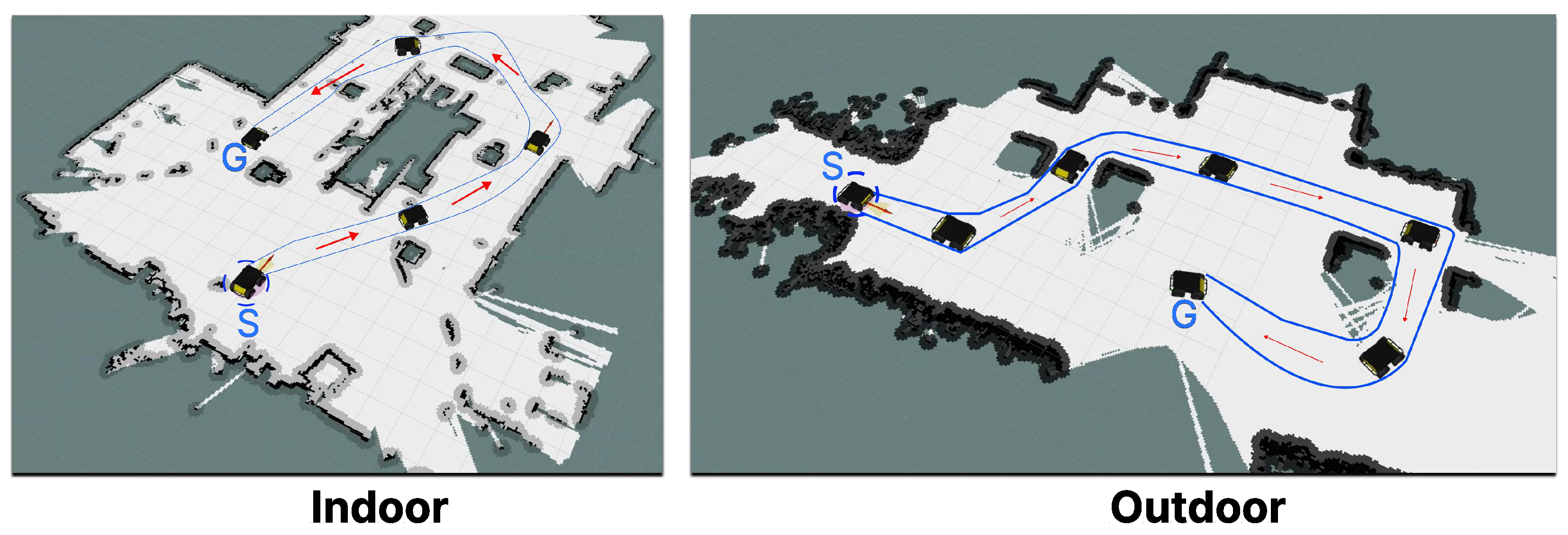
Figure 10 illustrates the navigation performance of the QSNE framework. The indoor scenario shows the robot starting at a blue circle, navigating a complex layout with static obstacles. The blue path with red arrows indicates successful traversal despite noise and flickering, with the PPO-LSTM processing degraded laser scans and the LLM providing semantic corrections. The outdoor scenario depicts the robot adapting to uneven terrain while maintaining a stable path through PQC-enhanced exploration and corrected LiDAR states.
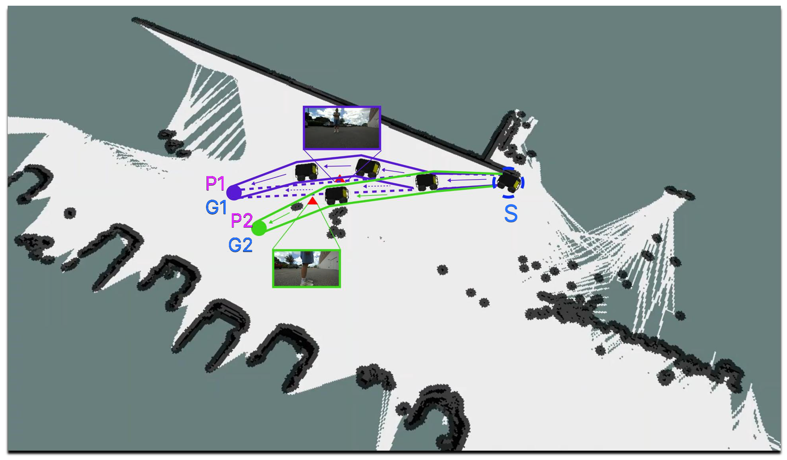
We extended the experimental validation to a dynamic parking lot environment, as shown in Figure 11. The Husky UGV navigates with human intervention to test the QSNE framework’s adaptability. In the P1 scenario, the detection of an obstacle at 1.5 m triggers the robot to stop, shift right, and continue, demonstrating effective obstacle avoidance. In the P2 scenario, an obstacle at 0.6 m prompts the robot to halt completely, preventing potential collisions. These responses rely on the QSNE’s sequential processing, semantic reasoning guidance, and quantum-enabled enhanced state correction.
Roughly 40% of failures occurred in the parking lot when a vehicle crossed at 8–10 m/s within one inter-trigger interval of the LLM module; the cached embedding e t described a stale obstacle configuration, and although the corrected scan s ^ t refreshed each control step, the higher-level recommendation lagged. A shorter trigger interval coupled with a local-model fallback would bound the round-trip latency and close this mode. A second pattern emerged in the Inspection and Construction Worlds when the robot remained near-stationary for over ∼20 s before a closed corridor or debris pile: the hidden state h t accumulated near-constant evidence, the corrected scan drifted toward an over-smoothed reconstruction that under-represented narrow openings, and the episode timed out on the step horizon. A reset of h t after a configurable idle period would address this without retraining. A third pattern occurred when 50% dropout removed nearly all rays in a single 30° sector for several consecutive scans: the sector statistics ( s ¯ t , k , σ t , k 2 , p k ) became extreme, the variance trigger fired in adjacent sectors, and the LLM occasionally recommended evasion into the blacked-out sector. An input-sanity filter that flags sectors with p k > 90 % as untrusted and rewrites the prompt is a planned improvement. A fourth pattern appeared near the goal in the Office World, where the Gaussian policy occasionally alternated forward and reverse commands under residual scan noise and missed the 0.5 m goal threshold within the step horizon; a larger goal-proximity reward or a separate 1 m terminal controller would suppress this, but neither was adopted here to preserve the simplicity of the reward function. No failure was attributable to PQC numerical instability, PPO clipped-objective divergence, or ROS connectivity loss, so the framework degrades along interpretable, component-specific modes rather than catastrophic collapse.

3.3. Ablation Studies and Component Analysis

To rigorously quantify the individual and synergistic contributions of the PQC and LLM modules, and to demonstrate that the reported performance gains are not solely attributable to the adoption of a recurrent reinforcement learning policy, we conducted a comprehensive ablation study. We trained and evaluated four controlled variants under identical conditions: the same 50% Gaussian noise (std = 2.0 m at 50% probability) + 50% ray-dropout degradation pipeline. Each variant was trained with 5 random seeds and evaluated over 10 trials per environment.
The variants include the following:
  • Standard PPO with 128-unit LSTM (no PQC, no LLM).
  • PQC (6 qubits, 4 layers) for quantum feature extraction only.
  • LLM semantic reasoning only (queries every 10 steps or when sector variance > 2.0).
  • Complete proposed QSNE framework (PPO + LSTM + PQC + LLM).
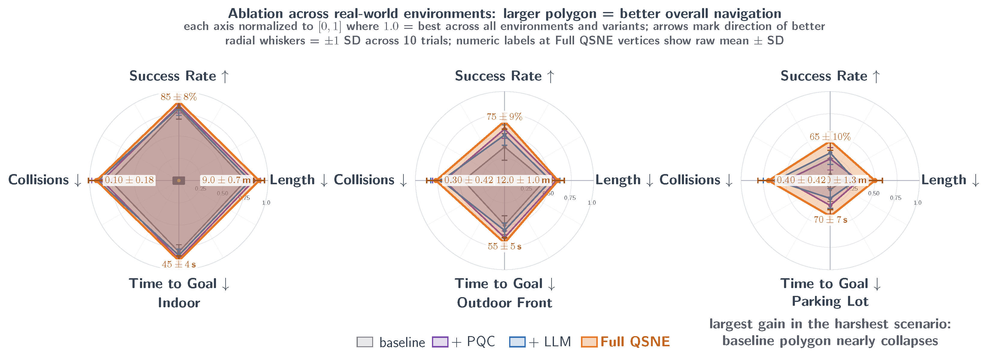
Figure 12 reports the navigation performance of all four variants across the three real-world environments. The results show clear additive and synergistic benefits. The PQC module consistently improves success rate and path efficiency. It delivers the largest gains in challenging outdoor and dynamic settings (for example, +9 pp success rate and 1.3 m shorter paths in the Outdoor Front environment). This outcome aligns with the quantum circuit ability to explore multiple probabilistic interpretations of noisy and flickering states in superposition. The LLM module substantially reduces collisions through semantic interpretation of degraded LiDAR data. It lowers collisions by up to 60% in the dynamic Parking Lot scenario. The full QSNE combination achieves the best overall performance. It yields synergistic improvements of 4–17 percentage points in success rate, 0.5–3.5 m shorter paths, and up to 67% fewer collisions compared with the ordinary PPO-LSTM baseline.
To further validate the framework under controlled but diverse conditions, we repeat the identical ablation suite in the four Gazebo simulation worlds (Inspection, Agriculture field, Office space, and Construction site). Table 6 reports the results. The trends mirror the real-world findings. The full QSNE achieves 14–17 percentage-point higher success rates and substantially shorter, safer trajectories across all simulated environments. These consistent sim-to-real gains confirm the robustness of the hybrid quantum-semantic enhancements.
We emphasize that the Gazebo worlds used here are substantially larger than the real-world sites and provide the larger-footprint evidence that physical experiments cannot. The Inspection World covers approximately 100 m × 80 m of hilly outdoor terrain with a cave, bridge, pipeline, and solar farm; the Agriculture World spans roughly 60 m × 60 m; the Construction World covers 50 m × 40 m of cluttered indoor space; and the Office World extends to 40 m × 30 m. The episodes in these worlds correspond to trajectory lengths of 35–90 m and step counts of 600–1400, and the QSNE advantages reported in Table 6 therefore hold over both larger spatial footprints and longer temporal horizons than the real-world campaign permits.
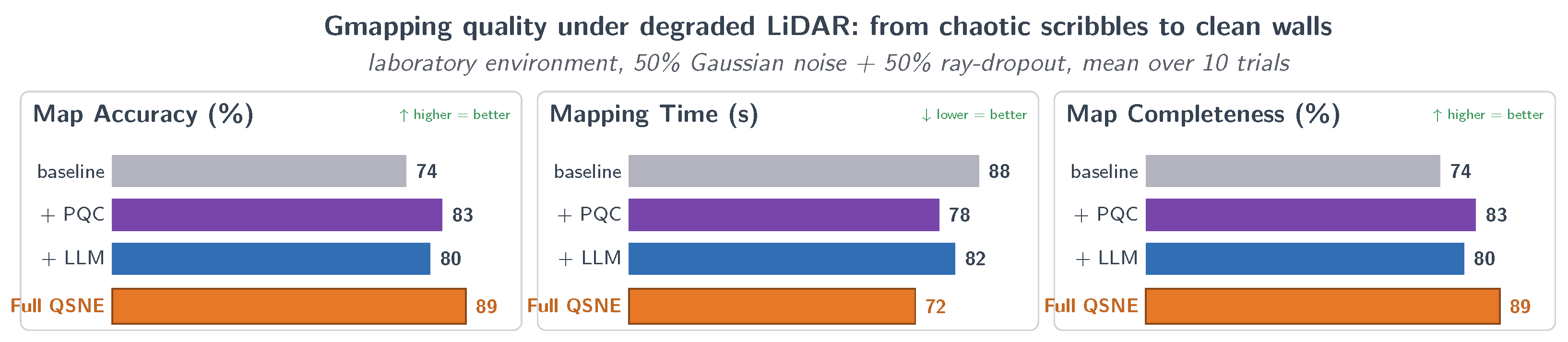
Figure 13 reports Gmapping performance on the laboratory environment (∼12 × 15 m) under the standard degradation. Full QSNE attains the best score on every metric (89% accuracy, 89% completeness, 72 s). PQC alone lifts accuracy 74→83% and cuts mapping time 88→78 s; LLM alone lifts accuracy 74→80% at 82 s. Table 7 gives the per-component contributions and synergy. PQC and LLM are toggled in the four variants and tabulated directly in Table 7. The LSTM contribution is given above: +8 pp success and −28% collisions when the policy receives LSTM-corrected versus raw scans, which is the same channel that drives map quality. The qubit-count sweep of Table 8 confirms the PQC contribution is monotonic up to six qubits, and the real-world (Figure 12) and Gazebo (Table 6) ablations reproduce the PQC > LLM > baseline ordering across seven further environments.
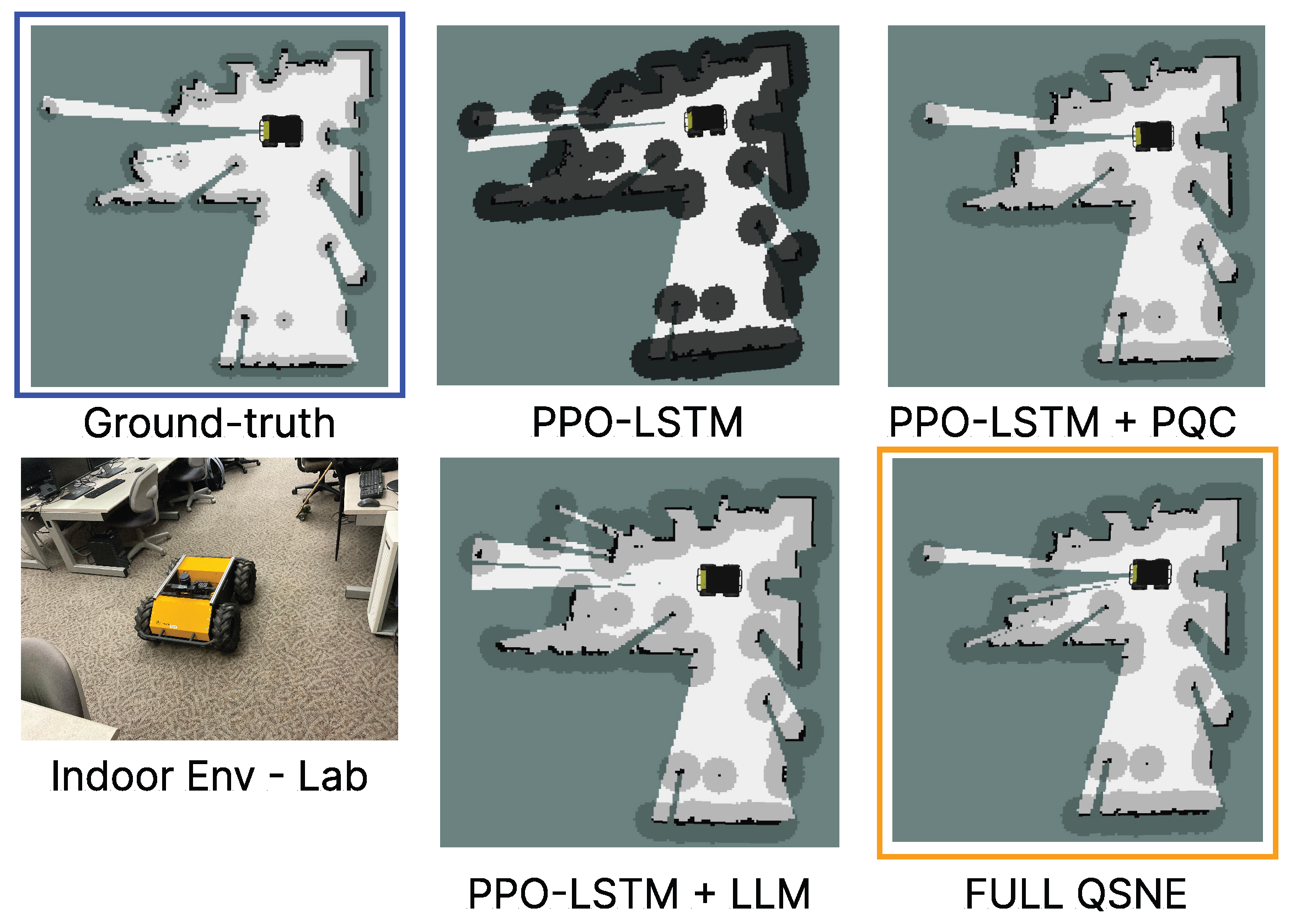
Figure 14 provides a visual comparison of the maps generated by Gmapping in the same laboratory environment. The ground-truth map appears in the top-left panel with a blue border. The real lab scene with the Husky UGV robot appears in the bottom-left panel. The remaining panels display the maps produced by the four ablation variants. The vanilla PPO-LSTM map contains heavy black noise clusters and distorted wall structures. The PPO-LSTM + PQC map reduces those artifacts in a significant manner and produces better wall alignment. The PPO-LSTM + LLM map recovers structural details but retains some residual gaps. The full QSNE map (bottom-right panel with orange border) approaches the ground-truth most closely. It exhibits sharp walls, minimal noise, and high overall fidelity. This visual evidence confirms the synergistic effect of the PQC and LLM modules on map reconstruction quality.
We further isolated the contribution of the LSTM-based point-cloud completion module s ^ t . We compared the vanilla PPO-LSTM agent on raw degraded scans against the same agent on corrected scans, averaged across the three real-world environments (10 trials each). With corrected scans, the success rate rises from 55% to 63% (+8 percentage points), the path length drops by 0.4 m, the time to goal drops by 4 s, and the collisions per trial drop from 0.95 to 0.68 (a 28% reduction). The LSTM temporal correction therefore provides cleaner observations to the policy. When this module is combined with PQC and LLM, the result is the full QSNE gain reported in Figure 12.
We examined the sensitivity of QSNE to the PQC width by sweeping the qubit count over { 4 , 6 , 8 } at a fixed depth of four layers on the indoor real-world environment (10 trials, PPO-LSTM + PQC variant). Table 8 reports the results. The four-to-six-qubit step delivers the largest success-rate improvement (+4 pp) at a modest 24% training-time cost; the six-to-eight-qubit step delivers a further 1 pp gain at a 31% training-time cost and a 38% inference-latency cost, both of which are consistent with the exponential simulation overhead of additional qubits. We therefore adopt six qubits as the default configuration. A complementary depth sweep at the chosen width is reported in Table 9 and confirms that four variational layers maximize success rate before training-time costs dominate.
To isolate the PQC contribution, the PQC encoder is swapped for two alternatives and the full PPO-LSTM pipeline is retrained under the standard degradation regime (50% Gaussian noise, σ = 2.0  m; 50% ray dropout; 10 trials, indoor). The first is a matched MLP ( 6 4 6 , 58 trainable parameters versus the 48 rotation parameters of the six-qubit, four-layer PQC). The second is a random-projection encoder with fixed Fourier features (non-learned reference). All three encoders feed identical LSTM, policy, and value heads.
Table 10 reports the comparison. The PQC achieves 83% success against 74% (MLP) and 61% (random projection), with matching reductions in path length and per-trial collisions. The PQC reaches the 80% threshold at ≈45k steps versus ≈78k for the MLP (a 42% reduction); the random-projection variant does not reach 80% within the 100k-step budget. Mean action-entropy over the first 30k steps is 1.42 nats (PQC) versus 1.18 nats (MLP), consistent with the Pauli-Z measurement stochasticity that drives early-training exploration. The PQC pays 7.1 ms inference latency versus the MLP’s 1.2 ms, an overhead expected to shrink on quantum hardware once simulation is removed.
To further demonstrate novelty against stronger baselines, we compared QSNE to recent learning-based methods for sensor degradation and POMDP navigation. The four modern baselines in Table 11 map onto the three families introduced in the literature review of Section 1.2. The first family is memory-augmented DRL for POMDPs, represented by LSTM-TD3 [28]. The second family is end-to-end DRL with a degradation-aware reward, represented by the perceived-risk crowd navigation method of Anas et al. [29], which embeds occupancy uncertainty into the reward to handle noise and flickering without an explicit map. The third family is modern SLAM backends with robustness features beyond Gmapping, represented by LIO-SAM [31] and by SLAM Toolbox [37], the modern pose-graph successor to Gmapping that runs on the same 2D LiDAR data as our pipeline. All four baselines were reproduced using open-source implementations and tested under our pipeline on the Husky UGV in the three real-world environments (10 trials each), under the same degradation pipeline (50% Gaussian noise with σ = 2.0  m and 50% ray dropout) as the QSNE evaluation. Table 11 reports average performance. QSNE achieves 11–19 pp higher success rates and up to 67% fewer collisions than these baselines, thanks to quantum-enhanced uncertainty modeling (PQC) and semantic reasoning (LLM) that better handle combined noise/flickering in POMDPs. This confirms novelty beyond standard DRL, as the baselines lack these hybrid elements.
Table 10. Comparison of the PQC encoder against classical encoders of matched parameter count on the indoor real-world environment (10 trials per configuration, mean ± standard deviation). All encoders output a six-dimensional feature vector and feed identical PPO-LSTM downstream pipelines, so the only varied component is the encoder itself. The “Steps to 80%” column reports the training step count at which the running success rate first reaches the 80% threshold; “n/a” indicates the threshold was not reached within the 100,000-step budget. The PQC reduces the step count to threshold by 42% relative to the matched MLP at comparable parameter count.
EncoderTrainable ParamsSuccess Rate (%)Path Length (m)Collisions/TrialSteps to 80%Inference (ms)
Random projection (6D)061 ± 1210.4 ± 1.20.55 ± 0.42n/a0.3
Classical MLP ( 6 4 6 )5874 ± 109.6 ± 0.90.34 ± 0.3078,0001.2
PQC (6 qubits, 4 layers)4883 ± 89.2 ± 0.70.20 ± 0.2145,0007.1
Table 11. Comparison to stronger learning-based baselines for sensor degradation and POMDP navigation (mean ± standard deviation over 10 trials across real-world environments). QSNE outperforms on all metrics; the paired-sample t-test against each baseline yields p < 0.01 on success rate and on collisions per trial (see Section 3.2).
MethodSuccess Rate (%)Path Length (m)Time to Goal (s)Collisions/Trial
LSTM-TD3 (POMDP baseline)58 ± 1314.0 ± 1.876 ± 110.82 ± 0.55
Deep RL Mapless Crowd Nav (degradation)64 ± 1113.2 ± 1.570 ± 90.55 ± 0.42
LIO-SAM (LiDAR fusion SLAM)61 ± 1213.6 ± 1.673 ± 100.68 ± 0.48
SLAM Toolbox [37] (pose-graph SLAM)60 ± 1313.5 ± 1.572 ± 90.66 ± 0.46
Full QSNE75 ± 911.3 ± 1.157 ± 60.27 ± 0.25

4. Conclusions

This paper proposes an integrative framework that addresses the critical limitations of traditional navigation algorithms in handling partial observability caused by degraded sensing data. The proposed approach enhances mobile robot navigation by incorporating adaptive state estimation, temporal feature fusion, semantic reasoning, and robust decision-making mechanisms to improve localization and mapping reliability in complex environments under partial observability. Experimental validation results confirmed that the framework outperforms the state-of-the-art AMCL and Gmapping across indoor, outdoor, and dynamic settings. Success rates rose from 20% to 65% in challenging parking lot scenarios, collisions dropped by 67%, and mapping errors decreased by 40%. These results stem from the system’s capability to correct distorted LiDAR states through quantum features and temporal processing, while semantic reasoning provides interpretable guidance for obstacle avoidance.
The real-world physical campaign was restricted to three campus sites of 15–25 m per side because larger outdoor sites approved for autonomous testing were not available, and because the Husky’s onboard battery and 2D LiDAR sensitivity to sunlight and reflective surfaces constrain extended outdoor operation. The contributions of this paper concern robustness to per-step sensor degradation over hundreds to thousands of degraded control steps, as well as the Gazebo campaign in Section 3.3. Validation in larger campus-scale and warehouse-scale physical environments with longer-horizon trajectories remains an important direction for future work, and we plan to pursue it as larger test sites become accessible.
The planar pose ( x t , y t , ϕ t ) in the observation vector d t introduces a translation and partial rotation dependence. The pose is expressed in the /odom frame, which the ROS stack initializes at the start of each episode, so the magnitudes of x t and y t at deployment are bounded by the episode trajectory rather than by an absolute global coordinate. The policy is nonetheless trained on trajectory extents matched to the spatial footprint of the three campus sites and four Gazebo worlds (approximately 15–100 m per side), and this train–test match limits the empirical evidence for cross-scale generalization. Deployment in substantially larger environments—multi-hundred-meter warehouse corridors or kilometer-scale outdoor traversals—would push ( x t , y t , ϕ t ) outside the support of the input distribution and can produce out-of-distribution decisions, even when the local LiDAR geometry remains representative of the trained regime. A principled remedy planned for subsequent work is to recast the policy input in a translation- and rotation-invariant form: the goal-relative range ρ g = p g p t and bearing β g in the robot body frame, the body-frame velocities ( v t , ω t ) , and the LiDAR scan s t , which is already body-fixed. This formulation removes the explicit ( x t , y t , ϕ t ) dependence, decouples the policy from the absolute extent of the test environment, and is the standard remedy in the map-less DRL navigation literature. The PQC and semantic-reasoning modules of QSNE are compatible with the invariant formulation without architectural change, since both consume only body-frame quantities at the input stage.
The contributions extend practical robotics by offering a modular enhancement that works alongside existing ROS tools without replacing the existing stack. Future work will explore scalability to multi-robot systems and integration with additional sensors like cameras for richer semantic understanding. Limitations include the computational demands of PQCs, which suggest opportunities for hardware acceleration on quantum processors. This novel navigation framework paves the way for safer, more adaptive ground robots in real-world applications such as disaster response and medical logistics.

Author Contributions

Conceptualization, T.N.H. and C.S.; methodology, T.N.H. and C.S.; software, T.N.H. and C.S.; validation, T.N.H. and C.S.; formal analysis, T.N.H., K.-D.N. and H.G.; investigation, T.N.H. and C.S.; resources, K.-D.N.; data curation, T.N.H. and C.S.; writing-original draft preparation, T.N.H., C.S. and K.-D.N.; writing–review and editing, T.N.H., K.-D.N. and H.G.; visualization, T.N.H. and C.S.; supervision, K.-D.N.; project administration, K.-D.N.; funding acquisition, K.-D.N. All authors have read and agreed to the published version of the manuscript.

Funding

This material is based upon work supported by the U.S. National Science Foundation under Grants #2138206 and #2245022.

Data Availability Statement

Data and implementation is available at https://github.com/huynhtnhut97/QSNE-Quantum-Semantic-Navigation-Enhancement (accessed on 22 June 2026).

Acknowledgments

The authors would like to thank the Florida Institute of Technology for providing access to the Husky UGV platform, the Gazebo simulation environment, and the High-Performance Computing (HPC) resources.

Conflicts of Interest

The authors declare no conflicts of interest.

References

  1. Sampedro, C.; Rodriguez-Ramos, A.; Bavle, H.; Carrio, A.; De la Puente, P.; Campoy, P. A fully-autonomous aerial robot for search and rescue applications in indoor environments using learning-based techniques. J. Intell. Robot. Syst. 2019, 95, 601–627. [Google Scholar]
  2. Kenk, M.A.; Hassaballah, M.; Brethé, J.F. Human-aware Robot Navigation in Logistics Warehouses. In Proceedings of the 16th International Conference on Informatics in Control, Automation and Robotics (ICINCO 2019), Prague, Czech Republic, 29–31 July 2019; pp. 371–378. [Google Scholar]
  3. Davidson, J.; Bhusal, S.; Mo, C.; Karkee, M.; Zhang, Q. Robotic manipulation for specialty crop harvesting: A review of manipulator and end-effector technologies. Glob. J. Agric. Allied Sci. 2020, 2, 25–41. [Google Scholar] [CrossRef]
  4. Ozkil, A.G.; Fan, Z.; Dawids, S.; Aanes, H.; Kristensen, J.K.; Christensen, K.H. Service robots for hospitals: A case study of transportation tasks in a hospital. In 2009 IEEE International Conference on Automation and Logistics; IEEE: New York, NY, USA, 2009; pp. 289–294. [Google Scholar]
  5. Ju, W. Application of autonomous navigation in robotics. In 2021 4th International Conference on Advanced Materials, Intelligent Manufacturing and Automation (AMIMA 2021), Hangzhou, China, 2–4 April 2021; Journal of Physics: Conference Series; IOP Publishing: Bristol, UK, 2021; Volume 1906, p. 012018. [Google Scholar]
  6. Jun, S.; Lee, S.; Yih, Y. Pickup and delivery problem with recharging for material handling systems utilising autonomous mobile robots. Eur. J. Oper. Res. 2021, 289, 1153–1168. [Google Scholar] [CrossRef]
  7. Schill, F.; Bahr, A.; Martinoli, A. Vertex: A new distributed underwater robotic platform for environmental monitoring. In Proceedings of the Distributed Autonomous Robotic Systems: The 13th International Symposium; Springer: Berlin/Heidelberg, Germany, 2018; pp. 679–693. [Google Scholar]
  8. Trevelyan, J.; Hamel, W.R.; Kang, S.C. Robotics in hazardous applications. In Springer Handbook of Robotics; Springer: Berlin/Heidelberg, Germany, 2016; pp. 1521–1548. [Google Scholar]
  9. Vargas, J.; Alsweiss, S.; Toker, O.; Razdan, R.; Santos, J. An overview of autonomous vehicles sensors and their vulnerability to weather conditions. Sensors 2021, 21, 5397. [Google Scholar] [CrossRef] [PubMed]
  10. Espinosa Peralta, P.; Luna, M.A.; de la Puente, P.; Campoy, P.; Bavle, H.; Carrio, A.; Cruz Ulloa, C. Performance analysis of localization algorithms for inspections in 2D and 3D unstructured environments using 3D laser sensors and UAVs. Sensors 2022, 22, 5122. [Google Scholar] [CrossRef] [PubMed]
  11. Gul, F.; Rahiman, W.; Nazli Alhady, S.S. A comprehensive study for robot navigation techniques. Cogent Eng. 2019, 6, 1632046. [Google Scholar] [CrossRef]
  12. Chen, P.; Zhao, X.; Zeng, L.; Liu, L.; Liu, S.; Sun, L.; Li, Z.; Chen, H.; Liu, G.; Qiao, Z. A review of research on slam technology based on the fusion of lidar and vision. Sensors 2025, 25, 1447. [Google Scholar] [CrossRef] [PubMed]
  13. Fan, Z.; Zhang, L.; Wang, X.; Shen, Y.; Deng, F. LiDAR, IMU, and camera fusion for simultaneous localization and mapping: A systematic review. Artif. Intell. Rev. 2025, 58, 174. [Google Scholar] [CrossRef]
  14. Li, Y.; An, J.; He, N.; Li, Y.; Han, Z.; Chen, Z.; Qu, Y. A Review of Simultaneous Localization and Mapping Algorithms Based on Lidar. World Electr. Veh. J. 2025, 16, 56. [Google Scholar] [CrossRef]
  15. Hu, Y.; Xie, F.; Yang, J.; Zhao, J.; Mao, Q.; Zhao, F.; Liu, X. Efficient Path Planning Algorithm Based on Laser SLAM and an Optimized Visibility Graph for Robots. Remote Sens. 2024, 16, 2938. [Google Scholar] [CrossRef]
  16. Bartal, I.; Özkurt, A. Performance of SLAM Algorithms According to Noise and Reduced Landmark Parameters. In 2023 14th International Conference on Electrical and Electronics Engineering (ELECO); IEEE: New York, NY, USA, 2023; pp. 1–5. [Google Scholar]
  17. Hodge, V.J.; Hawkins, R.; Alexander, R. Deep reinforcement learning for drone navigation using sensor data. Neural Comput. Appl. 2021, 33, 2015–2033. [Google Scholar]
  18. Huynh, T.N.; Nguyen, K.D. Integrative AI framework for robotics: LLM-enabled reinforcement learning in object manipulation and task planning. Robot. Auton. Syst. 2025, 195, 105197. [Google Scholar] [CrossRef]
  19. Spaan, M.T. Partially observable Markov decision processes. In Reinforcement learning: State-of-the-Art; Springer: Berlin/Heidelberg, Germany, 2012; pp. 387–414. [Google Scholar]
  20. Luo, W.; Wang, X.; Han, F.; Zhou, Z.; Cai, J.; Zeng, L.; Chen, H.; Chen, J.; Zhou, X. Research on LSTM-PPO Obstacle Avoidance Algorithm and Training Environment for Unmanned Surface Vehicles. J. Mar. Sci. Eng. 2025, 13, 479. [Google Scholar] [CrossRef]
  21. Wisniewski, M.; Chatzithanos, P.; Guo, W.; Tsourdos, A. Benchmarking deep reinforcement learning for navigation in denied sensor environments. arXiv 2024, arXiv:2410.14616. [Google Scholar]
  22. Lee, M.F.R.; Yusuf, S.H. Mobile robot navigation using deep reinforcement learning. Processes 2022, 10, 2748. [Google Scholar] [CrossRef]
  23. Zhu, K.; Zhang, T. Deep reinforcement learning based mobile robot navigation: A review. Tsinghua Sci. Technol. 2021, 26, 674–691. [Google Scholar] [CrossRef]
  24. Liu, Y.; Sun, Q.; Kapadia, D.R. Integrating Large Language Models into Robotic Autonomy: A Review of Motion, Voice, and Training Pipelines. AI 2025, 6, 158. [Google Scholar] [CrossRef]
  25. Xi, Z.; Chen, W.; Guo, X.; He, W.; Ding, Y.; Hong, B.; Zhang, M.; Wang, J.; Jin, S.; Zhou, E.; et al. The rise and potential of large language model based agents: A survey. Sci. China Inf. Sci. 2025, 68, 121101. [Google Scholar] [CrossRef]
  26. Sun, L.; Jha, D.K.; Hori, C.; Jain, S.; Corcodel, R.; Zhu, X.; Tomizuka, M.; Romeres, D. Interactive planning using large language models for partially observable robotic tasks. In 2024 IEEE International Conference on Robotics and Automation (ICRA); IEEE: New York, NY, USA, 2024; pp. 14054–14061. [Google Scholar]
  27. Tang, C.; Abbatematteo, B.; Hu, J.; Chandra, R.; Martín-Martín, R.; Stone, P. Deep reinforcement learning for robotics: A survey of real-world successes. In Proceedings of the AAAI Conference on Artificial Intelligence; AAAI Press: Palo Alto, CA, USA, 2025; Volume 39, pp. 28694–28698. [Google Scholar]
  28. Zhang, Q.; Zhang, L.; Ma, Q.; Xue, J. The LSTM-PER-TD3 algorithm for deep reinforcement learning in continuous control tasks. In 2023 China Automation Congress (CAC); IEEE: New York, NY, USA, 2023; pp. 671–676. [Google Scholar]
  29. Anas, H.; Hong, O.W.; Malik, O.A. Deep Reinforcement Learning-Based Mapless Crowd Navigation with Perceived Risk of the Moving Crowd for Mobile Robots. arXiv 2023, arXiv:2304.03593. [Google Scholar] [CrossRef]
  30. Wu, X.; Wei, C.; Guan, D.; Ji, Z. Risk-aware deep reinforcement learning for mapless navigation of unmanned surface vehicles in uncertain and congested environments. Ocean Eng. 2025, 322, 120446. [Google Scholar] [CrossRef]
  31. Shan, T.; Englot, B.; Meyers, D.; Wang, W.; Ratti, C.; Rus, D. Lio-sam: Tightly-coupled lidar inertial odometry via smoothing and mapping. In 2020 IEEE/RSJ International Conference on Intelligent Robots and Systems (IROS); IEEE: New York, NY, USA, 2020; pp. 5135–5142. [Google Scholar]
  32. Kim, D.; Lee, B.; Sung, S. Observability-driven path planning design for securing three-dimensional navigation performance of LiDAR SLAM. Aerospace 2023, 10, 492. [Google Scholar]
  33. Authors. Event-driven Control Approach of Cooperative Localization-Formation Hybrid for Internet of Multi-USV. IEEE Trans. Aerosp. Electron. Syst. 2026, 62, 5199–5212. [Google Scholar] [CrossRef]
  34. Fu, J.; Sun, G.; Yao, W.; Wu, C.; Wu, L. Dubins Path Planning of Heterogeneous UAV Collaborative Data Collection for IoT Network. IEEE Trans. Intell. Transp. Syst. 2026, 27, 2214–2224. [Google Scholar] [CrossRef]
  35. Shah, D.; Osiński, B.; Levine, S.; Levine, S. Lm-nav: Robotic navigation with large pre-trained models of language, vision, and action. In Proceedings of the Conference on Robot Learning, Auckland; PMLR; JMLR.org: Norfolk, MA, USA, 2022; pp. 492–504. [Google Scholar]
  36. Hohenfeld, H.; Heimann, D.; Wiebe, F.; Kirchner, F. Quantum deep reinforcement learning for robot navigation tasks. arXiv 2022, arXiv:2202.12180. [Google Scholar]
  37. Macenski, S.; Jambrecic, I. SLAM Toolbox: SLAM for the dynamic world. J. Open Source Softw. 2021, 6, 2783. [Google Scholar] [CrossRef]
Figure 1. Diagram of the QSNE framework. Degraded LiDAR(/noisy-scan) and odometry (/odom) feed a shared pipeline: PQC encoding, conditional LLM semantic embedding, and a 128-unit LSTM that maintains the latent state h t . Two heads diverge from h t : (right branch) a policy/value head that publishes the velocity command on /cmd_vel and is consumed by move_base as a local-planner override; (left branch) a scan-reconstruction decoder that publishes the corrected scan on /scan_corrected and is consumed by Gmapping to produce the corrected occupancy-grid map. The corrected map is then read back by the move_base costmap, closing the mapping–navigation loop. The two outputs are the final deliverables of the framework. Black dots represent raw LiDAR returns; red and white rays denote the sectorized and reduced scans, respectively. Solid arrows indicate data flow, while dashed boxes mark module boundaries and ROS-published outputs. Flicker (ray dropouts) refers to the LiDAR scan.
Robotics 15 00125 g001
Figure 2. Quantum-powered control agent pipeline. (1) Degraded LiDAR scans (noise + flicker) and odometry from the Husky form the observation o t R 725 . (2) A 6-qubit, 4-layer parameterized quantum circuit angle-encodes a normalized subset of o t , applies layered R-rotations and CNOT entanglers, and outputs measurement features f t = [ Z 1 , , Z 6 ] R 6 . (3) An unrolled LSTM (128 hidden units) integrates f t over time to produce the hidden state h t and a corrected scan s ^ t R 720 for Gmapping. (4) Fully-connected heads parameterize a Gaussian policy π ( a t | h t ) ; the clipped sample a t = [ v , ω ] is published on /cmd_vel to the localization module. The dashed arrow at the bottom denotes environment feedback to the next observation o t + 1 .
Robotics 15 00125 g002
Figure 3. Semantic reasoning integration: (A) The 720-ray LiDAR is compressed into a 12-sector summary Σ t R 36 of per-sector means, variances, and null fractions; sectors are color-coded by uncertainty level. A conditional gate (every 10 steps or when max k σ t , k 2 > τ ) decides whether to invoke the LLM, which trades semantic insight against computation cost. (B) The semantic reasoning module receives a structured prompt P combining Σ t and odometry d t , and returns a natural-language description D t that is encoded by a transformer into e t R 256 . (C) The embedding is concatenated with the PQC features f t to form i t = [ f t , e t ] R 262 , the augmented input to the learning-control agent. Solid arrows indicate data flow; orange/gray arrows denote query gating; purple arrows represent feature fusion; and the green arrow feeds the LSTM agent. Dashed rings are LiDAR range guides, and the red/gray callouts mark the high-variance and fully-null sectors.
Robotics 15 00125 g003
Figure 4. Visual representation of Gazebo-simulated environments from the Clearpath Gazebo Worlds collection, including Inspection World (hilly outdoor with cave), Agriculture World (flat outdoor with barn), Office World (indoor with furniture), and Construction World (indoor with debris). The red/green/blue lines in the Inspection World represent the X, Y, and Z axes of the origin point.
Robotics 15 00125 g004
Figure 5. Training progress of the proposed QSNE agent in Gazebo simulations. The plot tracks average episodic reward (blue), success rate (red), and steps to goal (green) over 100,000 time steps, with smoothed curves revealing consistent improvement.
Robotics 15 00125 g005
Figure 6. Experiments in real-world environments, including the indoor building (15 m × 15 m office with furniture), the outdoor front of the building (20 m × 20 m area with trees and pedestrians), and the parking lot (25 m × 25 m with cars and vehicles).
Robotics 15 00125 g006
Figure 7. Partial observability effects on AMCL (a traditional method) in the indoor environment. The left image shows the pre-mapped 2D map with a blue circle marking the robot’s starting position. The right three columns depict the following: (1) noise causing navigation failure through a narrow path due to the robot perceiving obstacles as closer, (2) sensor flickering misaligning the robot’s map position into the stairs obstacle, and (3) their combination resulting in collisions with a shifted position. The red arrow indicates the direction that the Husky is facing.
Robotics 15 00125 g007
Figure 8. Partial observability effects on AMCL (a traditional method) in an outdoor environment. The left image shows the pre-mapped 2D map with a blue circle marking the robot’s starting position. The right three columns each display a zoomed region of the map where the robot failed to navigate, paired with the robot’s corresponding point of view, depicting the following: (1) noise causing the robot to stop moving after advancing despite distant obstacles due to excessive range uncertainty triggering a safety stop or perceived self-collision, (2) sensor flickering shifting the robot’s map position into the pillar obstacle, and (3) their combination resulting in a longer path to the destination. The red arrow indicates the direction that the Husky is facing.
Robotics 15 00125 g008
Figure 9. Effect of noise, flickering, and their combination on Gmapping maps (first three columns). Rows represent indoor and outdoor environments. Columns show noise, flickering, combination, ground-truth, and QSNE results, highlighting improved map accuracy with the QSNE framework. The black dots represent raw sensor data points captured by the robot’s lidar. These dots indicate detected obstacles or surfaces within the robot’s field of view. Each panel carries three on-figure annotations: a 5 m scale bar in the lower-left corner; a north-arrow marker in the upper-right corner; and a metric overlay in the upper-left corner that reports the map error (Err, in meters), the map completeness (Cmp, in percent), and the structural similarity index (SSIM) against the ground-truth map of the matching row. Blue and orange boxes show the ground-truth and QSNE results.
Robotics 15 00125 g009
Figure 10. Navigation paths of the Husky UGV using the proposed QSNE framework under partial observability. In each panel, a blue character labeled ‘S’ marks the start position and ‘G’ marks the goal. The (left) image shows the indoor environment with a blue starting circle and a blue path with red arrows. The red arrow indicates the direction that the Husky is facing. The (right) image displays the outdoor environment with similar markings.
Robotics 15 00125 g010
Figure 11. Navigation paths in the dynamic parking lot with human intervention. A blue character labeled ‘S’ marks the start position, and ‘G’ marks the goal. The image shows the robot’s starting position (blue circle), paths from P1 and P2, and inset views of human obstacles. P1 illustrates a right shift at 1.5 m, while P2 shows a stop at 2 feet. The red triangles show the pedestrian positions. The dashed purple line is the planned path to P1; the solid purple arrows trace the actual path, which detours around the first pedestrian after detection. The solid green arrows trace the path toward P2 and terminate where a second pedestrian stepped into the lane at close range and prompted a full stop. The purple and green photo insets show the on-board camera view of each pedestrian.
Robotics 15 00125 g011
Figure 12. Real-world ablation, drawn as polar plots with one panel per environment and four metric axes per panel. Each axis is normalized to [ 0 , 1 ] , where 1.0 is the best value observed across all environments and variants; lower-is-better metrics are inverted, so a larger polygon indicates better overall navigation. Full QSNE (orange) encloses the other variants in every environment. The gap is largest in the Parking Lot, where the ordinary PPO-LSTM polygon contracts to near the centre. Means over 10 trials per environment under 50% Gaussian noise (std = 2.0 m) and 50% ray dropout. The ↑ on Success Rate marks higher-is-better; the ↓ on Length, Time to Goal, and Collisions marks lower-is-better. All four axes are normalized to [ 0 , 1 ] , so a larger polygon area indicates a better overall result on every metric.
Robotics 15 00125 g012
Figure 13. Gmapping reconstruction quality in the laboratory environment under 50% Gaussian noise and 50% ray dropout (mean over 10 trials). The three panels report map accuracy, mapping time, and map completeness for the four ablation variants. The full QSNE achieves 89% map accuracy and 89% completeness with a mapping time of 72 s, the best result on every metric. The per-component decomposition of the result is reported in Table 7.
Robotics 15 00125 g013
Figure 14. Comparison of generated maps in the indoor laboratory environment. The ground-truth map (top-left, blue border) serves as reference. The real lab environment with the Husky UGV appears in the bottom-left. Maps from the four ablation variants demonstrate progressive improvement. The full QSNE (bottom-right, orange border) achieves the highest fidelity to the ground-truth.
Robotics 15 00125 g014
Table 1. Per-component inference time, hardware location, and real-time impact of each module in the QSNE pipeline. Frequencies are expressed relative to the 10 Hz control loop. The LLM call is the only component that runs off-board, and the asynchronous ROS architecture prevents it from blocking the control loop. The LLM latency in this table is the mean ± standard deviation over 1000 deployment calls collected across the full real-world scenario.
ComponentHardwareInference TimeCall FrequencyBlocks Control Loop?
PPO-LSTM policy + value headOnboard CPU (i7-12700H) 8.2 ± 1.1  msEvery step (10 Hz)Yes (within 100 ms budget)
Scan-reconstruction decoderOnboard CPU 4.1 ± 0.6  msEvery step (10 Hz)Yes (within 100 ms budget)
PQC (6 qubits, 4 layers)Onboard CPU (PennyLane) 7.1 ± 0.9  msEvery step (10 Hz)Yes (within 100 ms budget)
Transformer encoder (DistilBERT)Onboard CPU 12 ± 2  msPer LLM response (≈1.3 Hz)No (asynchronous node)
GPT-4o API callCloud (OpenAI, campus Wi-Fi) 780 ± 220  msOnce per 10 steps or on σ t , k 2 > τ No (asynchronous node)
Total on-board per stepOnboard CPU 19 . 4 ± 2 . 6  msEvery step (10 Hz)19.4 ms of 100 ms budget
Table 2. End-to-end latency profile of the semantic-reasoning module, reported as median and 95th-percentile ( p 95 ) over 500 controlled indoor profiling calls with the hosted GPT-4o API. This corresponds to a per-stage breakdown of the LLM latency in Table 1, which reports the mean ± standard deviation over the full 1000-call deployment campaign. The aggregate latency exceeds the 100 ms control-loop budget by roughly a factor of six and motivates the asynchronous execution mode described in Section 2.4.
ComponentMedian (ms) p 95 (ms)Share of Median (%)
Prompt assembly1.82.60.3
GPT-4o round trip612141098.9
Response parsing0.91.40.1
Transformer encoding ( D t e t )4.26.10.7
Total6191420100.0
Table 3. QSNE hyperparameters. The table is grouped in four blocks: PPO training, LSTM and policy/value heads, PQC, and LLM and semantic reasoning. Values were either taken from the original references or selected via the sensitivity sweeps reported in Section 3.3.
BlockHyperparameter (Symbol)ValueRationale/Source
PPO trainingTotal time steps 10 5 Convergence point in training progress
Learning rate 3 × 10 4 Standard PPO default
Batch size64Standard PPO default
Entropy coefficient 10 2 Encourages exploration under degradation
Clip parameter ( ϵ ) 0.2 Schulman et al. PPO recommendation
Discount factor ( γ ) 0.99 Standard long-horizon value
GAE λ 0.95 Standard PPO default
LSTM + headsLSTM hidden units128Capacity sufficient for 720-ray temporal context
Policy/value FC layers 2 × 64 Matches Stable Baselines3 default
Action space (clipped) v [ 0 , 2.0 ] m/s, ω [ 1.0 , 1.0 ] rad/sHusky UGV velocity limits
Initial action std ( σ t ) [ 0.1 , 0.05 ] Tuned empirically
PQCNumber of qubits6Selected via PQC qubit-count
Number of variational layers4Selected via PQC depth
Rotation gates R X , R Y Angle-encoding standard
Entangling gatesCNOT (linear chain)Nearest-neighbor entanglement
Measurement basisPauli-Z per qubitYields f t R 6
LLM + reasoningBackboneGPT-4oHosted API
Sector count1230° per sector, balances detail vs. prompt size
Embedding dimension ( e t )256Transformer encoder output
Query interval (steps)10Balances responsiveness and API cost
Variance trigger threshold ( τ ) 2.0 Matches noise std; triggers reasoning under uncertainty
Model snapshotgpt-4o-2024-08-06Frozen version pin; no fine-tuning
Execution modeAsynchronous, background threadDecouples 619 ms LLM RTT from 100 ms control budget
Table 4. Performance comparison for AMCL with and without the hybrid framework in real-world environments (10 trials each); values reported as mean ± standard deviation. The QSNE standard deviations are smaller than AMCL’s on every metric in every environment, which indicates a more stable system. The associated 95% confidence half-widths and the rationale for the 10-trial protocol are stated at the start of Section 3.2.
EnvironmentSuccess Rate (%)Path Length (m)Time to Goal (s)Collisions/Trial
Indoor Environment (AMCL)80 ± 1310.5 ± 1.450 ± 70.3 ± 0.5
Indoor Env. (our method: QSNE)85 ± 89.0 ± 0.745 ± 40.1 ± 0.3
Outdoor Front (AMCL)55 ± 1513.5 ± 2.065 ± 100.7 ± 0.6
Outdoor Front (QSNE)75 ± 912.0 ± 1.055 ± 50.3 ± 0.4
Parking Lot (AMCL)20 ± 1816.5 ± 2.985 ± 141.2 ± 0.9
Parking Lot (QSNE)65 ± 1013.0 ± 1.370 ± 70.4 ± 0.4
Table 5. Performance comparison of QSNE versus Gmapping in real-world environments (10 trials each); values reported as mean ± standard deviation. The associated 95% confidence half-widths and the rationale for the 10-trial protocol are stated at the start of Section 3.2.
EnvironmentMap Error (m)Mapping Time (s)Map Completeness (%)
Indoor Environment (Gmapping)0.8 ± 0.1890 ± 1270 ± 9
Indoor Env. (QSNE)0.5 ± 0.0975 ± 785 ± 5
Outdoor Front (Gmapping)1.0 ± 0.25100 ± 1565 ± 11
Outdoor Front (QSNE)0.6 ± 0.1285 ± 880 ± 6
Parking Lot (Gmapping)1.5 ± 0.42120 ± 2250 ± 14
Parking Lot (QSNE)0.9 ± 0.1895 ± 1070 ± 7
Table 6. Ablation results—Gazebo simulation worlds (mean ± standard deviation over 10 trials per world).
EnvironmentVariantSuccess Rate (%)Path Length (m)Time to Goal (s)Collisions/Trial
InspectionPPO-LSTM65 ± 1413.8 ± 1.778 ± 110.55 ± 0.42
PPO-LSTM + PQC74 ± 1112.1 ± 1.368 ± 80.32 ± 0.31
PPO-LSTM + LLM71 ± 1212.5 ± 1.472 ± 90.28 ± 0.28
Full QSNE82 ± 810.9 ± 0.962 ± 60.15 ± 0.18
AgriculturePPO-LSTM82 ± 1011.5 ± 1.264 ± 80.35 ± 0.30
PPO-LSTM + PQC90 ± 710.2 ± 0.956 ± 60.20 ± 0.21
PPO-LSTM + LLM87 ± 810.6 ± 1.059 ± 70.18 ± 0.19
Full QSNE96 ± 59.4 ± 0.651 ± 40.10 ± 0.12
OfficePPO-LSTM88 ± 89.8 ± 0.955 ± 60.25 ± 0.24
PPO-LSTM + PQC93 ± 68.7 ± 0.748 ± 50.15 ± 0.16
PPO-LSTM + LLM91 ± 79.1 ± 0.751 ± 50.12 ± 0.14
Full QSNE98 ± 38.2 ± 0.545 ± 30.08 ± 0.10
ConstructionPPO-LSTM72 ± 1313.1 ± 1.674 ± 100.52 ± 0.40
PPO-LSTM + PQC80 ± 911.6 ± 1.265 ± 70.32 ± 0.28
PPO-LSTM + LLM78 ± 1012.0 ± 1.368 ± 80.28 ± 0.27
Full QSNE88 ± 610.5 ± 0.858 ± 50.18 ± 0.20
Table 7. Per-component contribution to the laboratory mapping experiment of Figure 13. Marginal contribution is reported as the change relative to the PPO-LSTM baseline. Relative share is the marginal contribution expressed as a percentage of the total gain achieved by the full QSNE. The synergy row reports the difference between the full-QSNE gain and the arithmetic sum of the individual PQC and LLM marginal contributions; the near-zero values indicate that the two components combine in an approximately additive manner on these three map-quality metrics.
Variant/ContributionMap Accuracy (%) Δ Acc (pp)Mapping Time (s) Δ Time (s)Completeness (%) Δ Comp (pp)
Baseline (PPO&LSTM)748874
+PQC (marginal)83+978−1083+9
+LLM (marginal)80+682−680+6
Full QSNE (PPO&LSTM + PQC + LLM)89+1572−1689+15
Relative share of full gain—PQC60%63%60%
Relative share of full gain—LLM40%37%40%
Synergy (full − PQC − LLM)000
Table 8. PQC qubit-count sweep at fixed depth of four layers (PPO-LSTM + PQC variant, indoor real-world environment, 10 trials per configuration, mean ± standard deviation).
QubitsSuccess Rate (%)Path Length (m)Training Time (min)Inference Latency (ms)
479 ± 109.6 ± 0.9425.1
6 (default)83 ± 89.2 ± 0.7527.1
884 ± 89.1 ± 0.7689.8
Table 9. PQC depth sweep at fixed width of six qubits (PPO-LSTM + PQC variant, indoor real-world environment, 10 trials per configuration, mean ± standard deviation). Four layers maximize success rate; deeper circuits show diminishing returns and substantially higher training cost.
LayersSuccess Rate (%)Path Length (m)Training Time (min)Inference Latency (ms)
278 ± 119.7 ± 0.9384.6
4 (default)83 ± 89.2 ± 0.7527.1
683 ± 99.2 ± 0.87410.4
Disclaimer/Publisher’s Note: The statements, opinions and data contained in all publications are solely those of the individual author(s) and contributor(s) and not of MDPI and/or the editor(s). MDPI and/or the editor(s) disclaim responsibility for any injury to people or property resulting from any ideas, methods, instructions or products referred to in the content.