Figure 1.
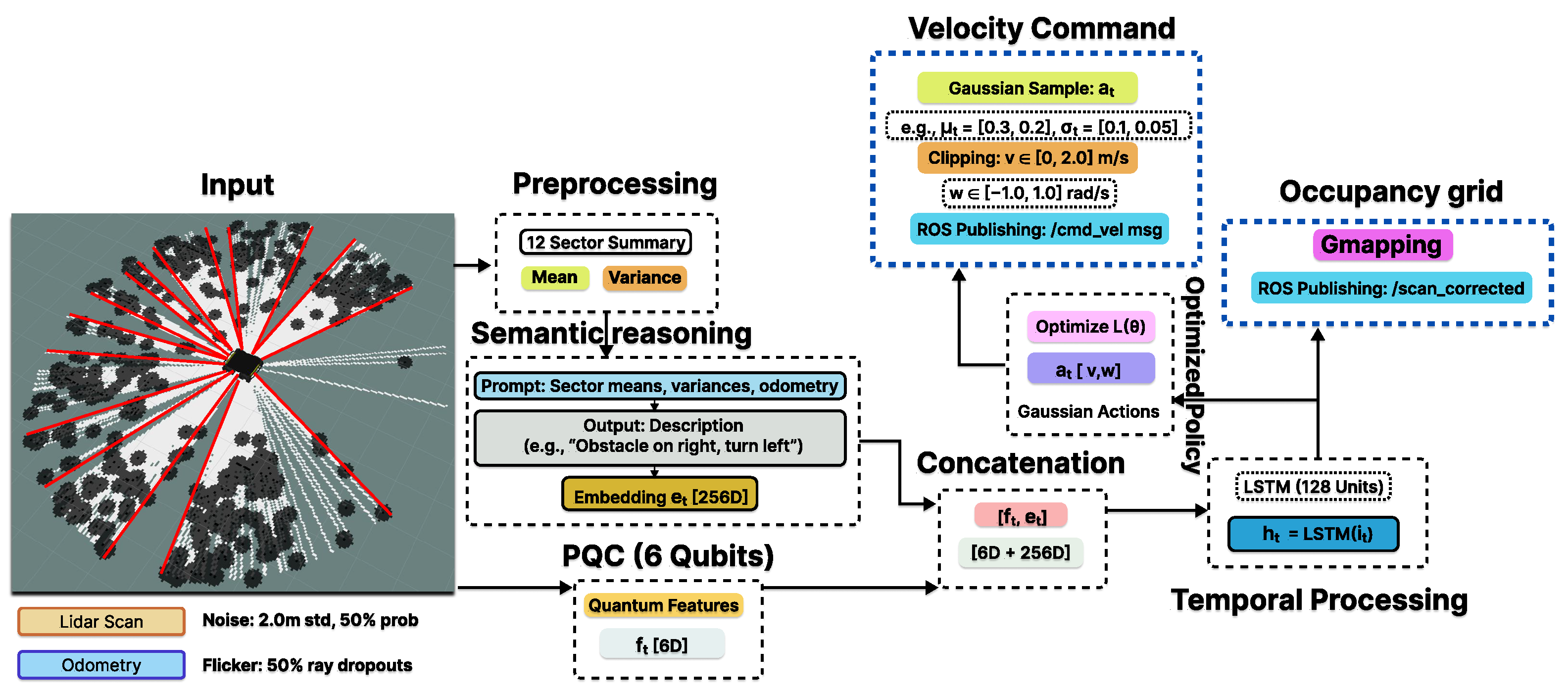
Diagram of the QSNE framework. Degraded LiDAR(/noisy-scan) and odometry (/odom) feed a shared pipeline: PQC encoding, conditional LLM semantic embedding, and a 128-unit LSTM that maintains the latent state . Two heads diverge from : (right branch) a policy/value head that publishes the velocity command on /cmd_vel and is consumed by move_base as a local-planner override; (left branch) a scan-reconstruction decoder that publishes the corrected scan on /scan_corrected and is consumed by Gmapping to produce the corrected occupancy-grid map. The corrected map is then read back by the move_base costmap, closing the mapping–navigation loop. The two outputs are the final deliverables of the framework. Black dots represent raw LiDAR returns; red and white rays denote the sectorized and reduced scans, respectively. Solid arrows indicate data flow, while dashed boxes mark module boundaries and ROS-published outputs. Flicker (ray dropouts) refers to the LiDAR scan.
Figure 1.
Diagram of the QSNE framework. Degraded LiDAR(/noisy-scan) and odometry (/odom) feed a shared pipeline: PQC encoding, conditional LLM semantic embedding, and a 128-unit LSTM that maintains the latent state . Two heads diverge from : (right branch) a policy/value head that publishes the velocity command on /cmd_vel and is consumed by move_base as a local-planner override; (left branch) a scan-reconstruction decoder that publishes the corrected scan on /scan_corrected and is consumed by Gmapping to produce the corrected occupancy-grid map. The corrected map is then read back by the move_base costmap, closing the mapping–navigation loop. The two outputs are the final deliverables of the framework. Black dots represent raw LiDAR returns; red and white rays denote the sectorized and reduced scans, respectively. Solid arrows indicate data flow, while dashed boxes mark module boundaries and ROS-published outputs. Flicker (ray dropouts) refers to the LiDAR scan.
Figure 2.
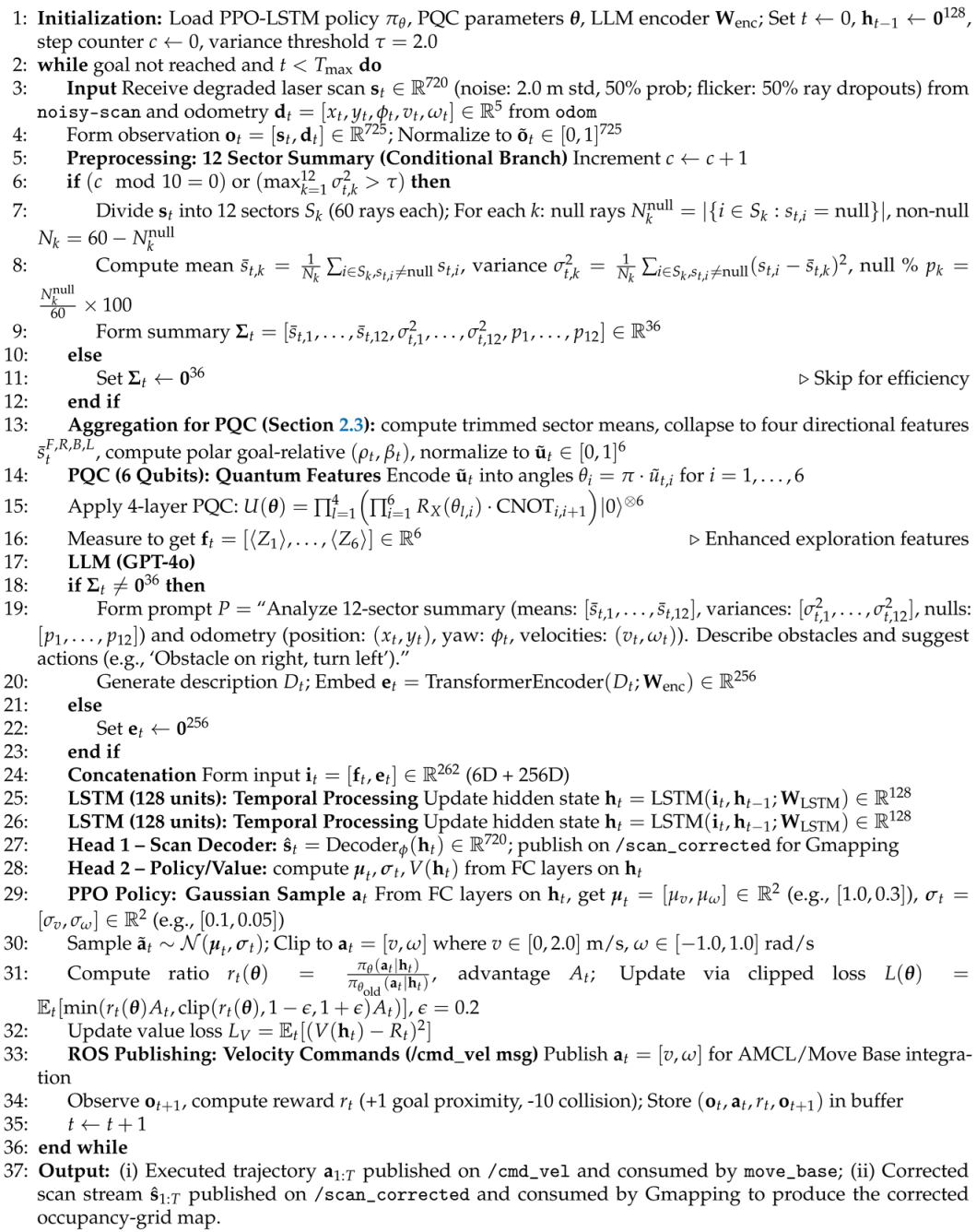
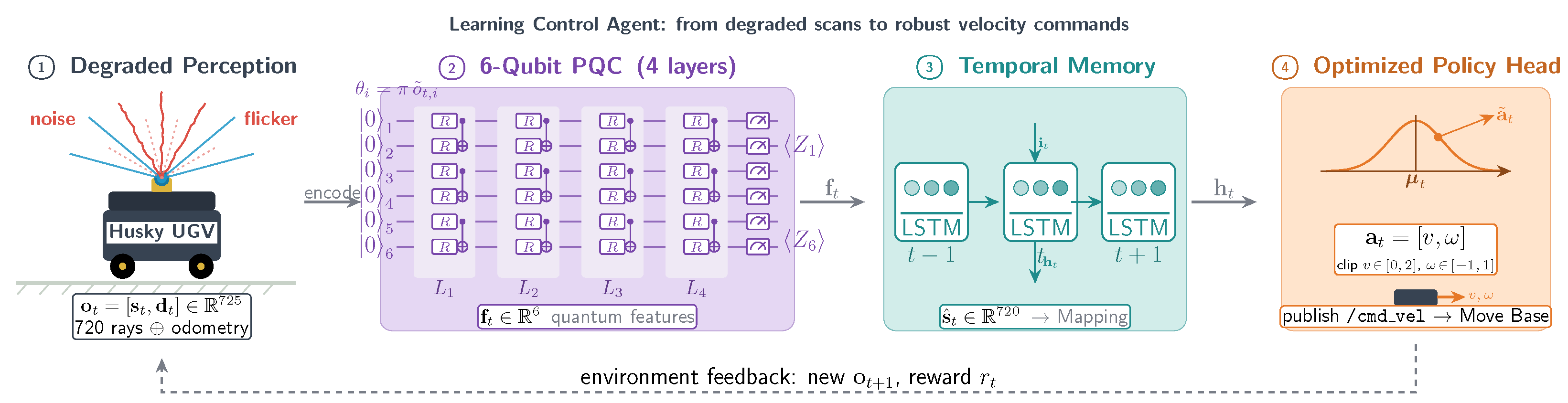
Quantum-powered control agent pipeline. (1) Degraded LiDAR scans (noise + flicker) and odometry from the Husky form the observation . (2) A 6-qubit, 4-layer parameterized quantum circuit angle-encodes a normalized subset of , applies layered R-rotations and CNOT entanglers, and outputs measurement features . (3) An unrolled LSTM (128 hidden units) integrates over time to produce the hidden state and a corrected scan for Gmapping. (4) Fully-connected heads parameterize a Gaussian policy ; the clipped sample is published on /cmd_vel to the localization module. The dashed arrow at the bottom denotes environment feedback to the next observation .
Figure 2.
Quantum-powered control agent pipeline. (1) Degraded LiDAR scans (noise + flicker) and odometry from the Husky form the observation . (2) A 6-qubit, 4-layer parameterized quantum circuit angle-encodes a normalized subset of , applies layered R-rotations and CNOT entanglers, and outputs measurement features . (3) An unrolled LSTM (128 hidden units) integrates over time to produce the hidden state and a corrected scan for Gmapping. (4) Fully-connected heads parameterize a Gaussian policy ; the clipped sample is published on /cmd_vel to the localization module. The dashed arrow at the bottom denotes environment feedback to the next observation .
Figure 3.
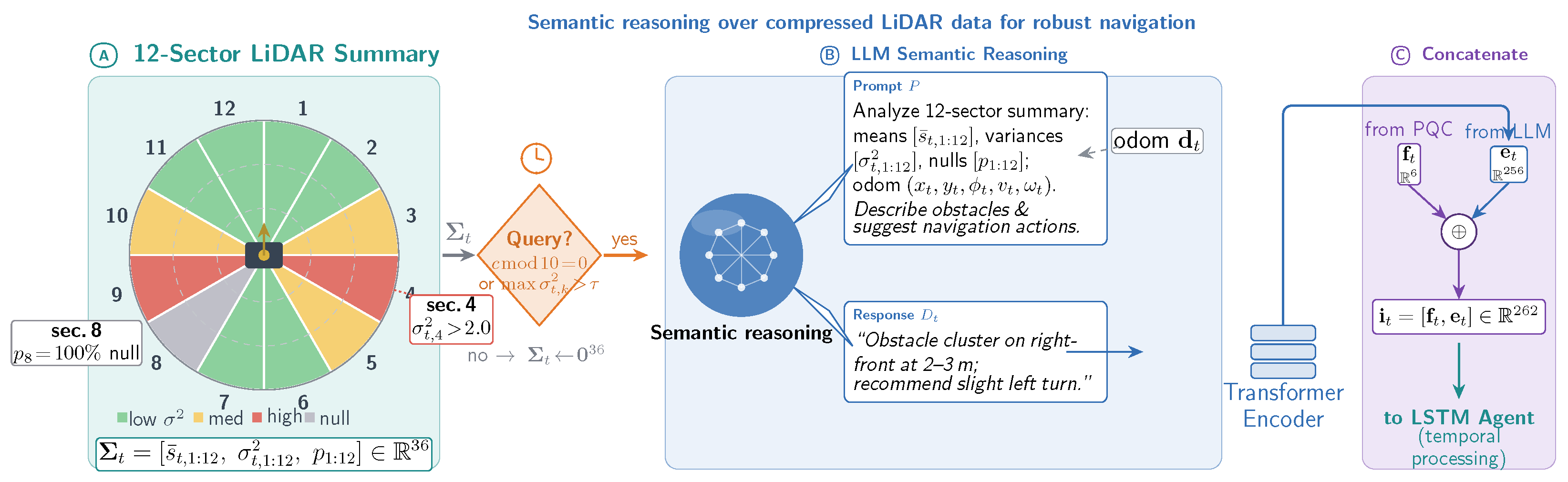
Semantic reasoning integration: (A) The 720-ray LiDAR is compressed into a 12-sector summary of per-sector means, variances, and null fractions; sectors are color-coded by uncertainty level. A conditional gate (every 10 steps or when ) decides whether to invoke the LLM, which trades semantic insight against computation cost. (B) The semantic reasoning module receives a structured prompt P combining and odometry , and returns a natural-language description that is encoded by a transformer into . (C) The embedding is concatenated with the PQC features to form , the augmented input to the learning-control agent. Solid arrows indicate data flow; orange/gray arrows denote query gating; purple arrows represent feature fusion; and the green arrow feeds the LSTM agent. Dashed rings are LiDAR range guides, and the red/gray callouts mark the high-variance and fully-null sectors.
Figure 3.
Semantic reasoning integration: (A) The 720-ray LiDAR is compressed into a 12-sector summary of per-sector means, variances, and null fractions; sectors are color-coded by uncertainty level. A conditional gate (every 10 steps or when ) decides whether to invoke the LLM, which trades semantic insight against computation cost. (B) The semantic reasoning module receives a structured prompt P combining and odometry , and returns a natural-language description that is encoded by a transformer into . (C) The embedding is concatenated with the PQC features to form , the augmented input to the learning-control agent. Solid arrows indicate data flow; orange/gray arrows denote query gating; purple arrows represent feature fusion; and the green arrow feeds the LSTM agent. Dashed rings are LiDAR range guides, and the red/gray callouts mark the high-variance and fully-null sectors.
Figure 4.
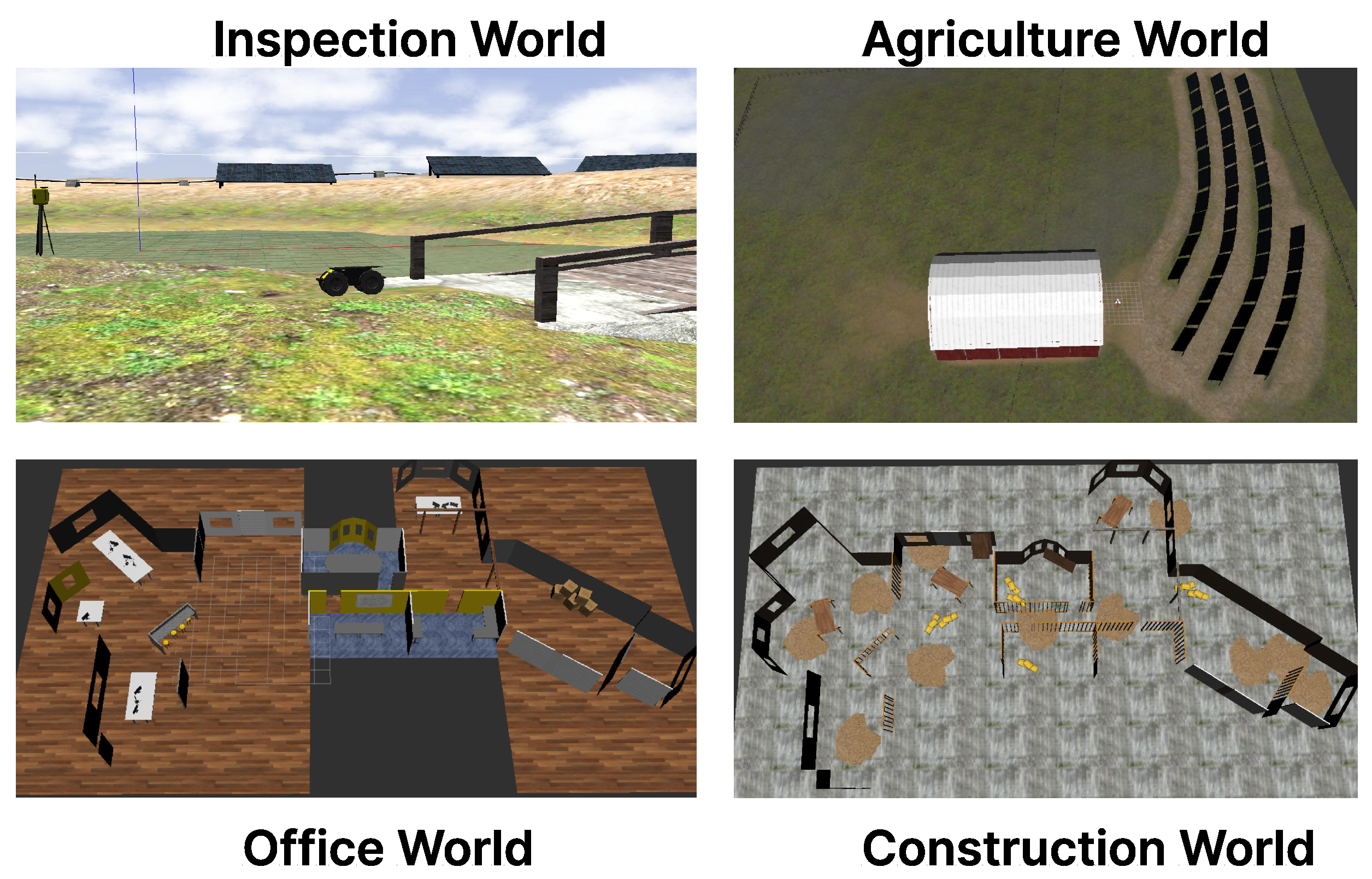
Visual representation of Gazebo-simulated environments from the Clearpath Gazebo Worlds collection, including Inspection World (hilly outdoor with cave), Agriculture World (flat outdoor with barn), Office World (indoor with furniture), and Construction World (indoor with debris). The red/green/blue lines in the Inspection World represent the X, Y, and Z axes of the origin point.
Figure 4.
Visual representation of Gazebo-simulated environments from the Clearpath Gazebo Worlds collection, including Inspection World (hilly outdoor with cave), Agriculture World (flat outdoor with barn), Office World (indoor with furniture), and Construction World (indoor with debris). The red/green/blue lines in the Inspection World represent the X, Y, and Z axes of the origin point.
Figure 5.
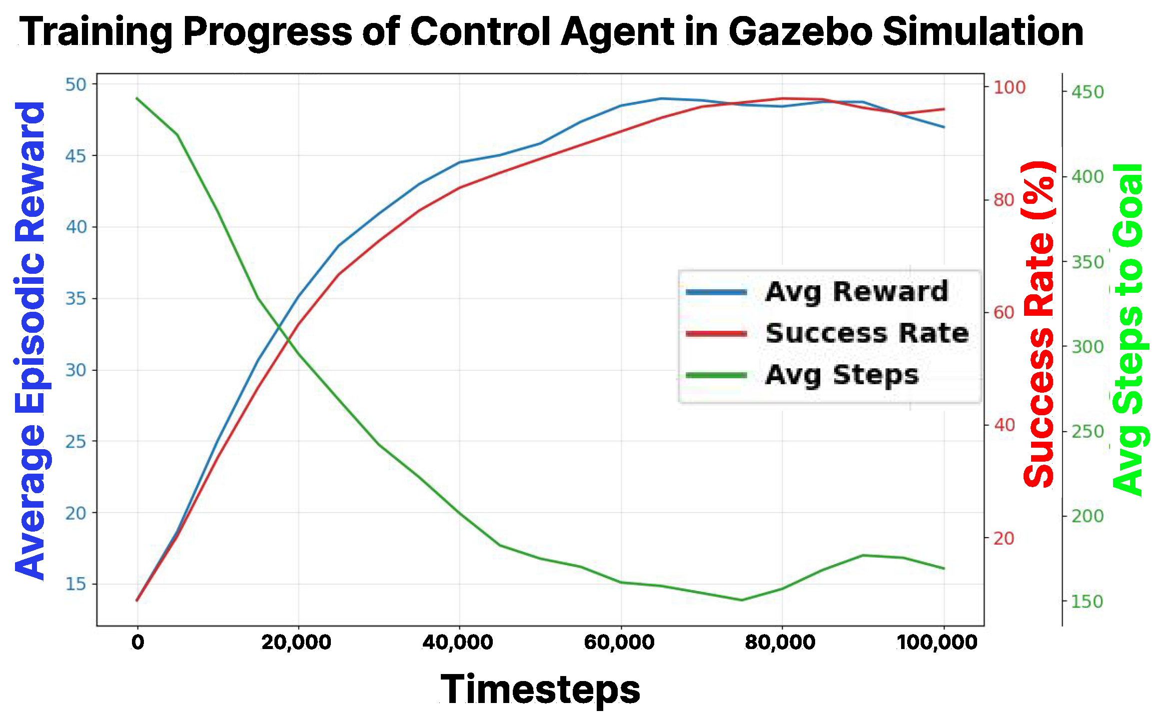
Training progress of the proposed QSNE agent in Gazebo simulations. The plot tracks average episodic reward (blue), success rate (red), and steps to goal (green) over 100,000 time steps, with smoothed curves revealing consistent improvement.
Figure 5.
Training progress of the proposed QSNE agent in Gazebo simulations. The plot tracks average episodic reward (blue), success rate (red), and steps to goal (green) over 100,000 time steps, with smoothed curves revealing consistent improvement.
Figure 6.
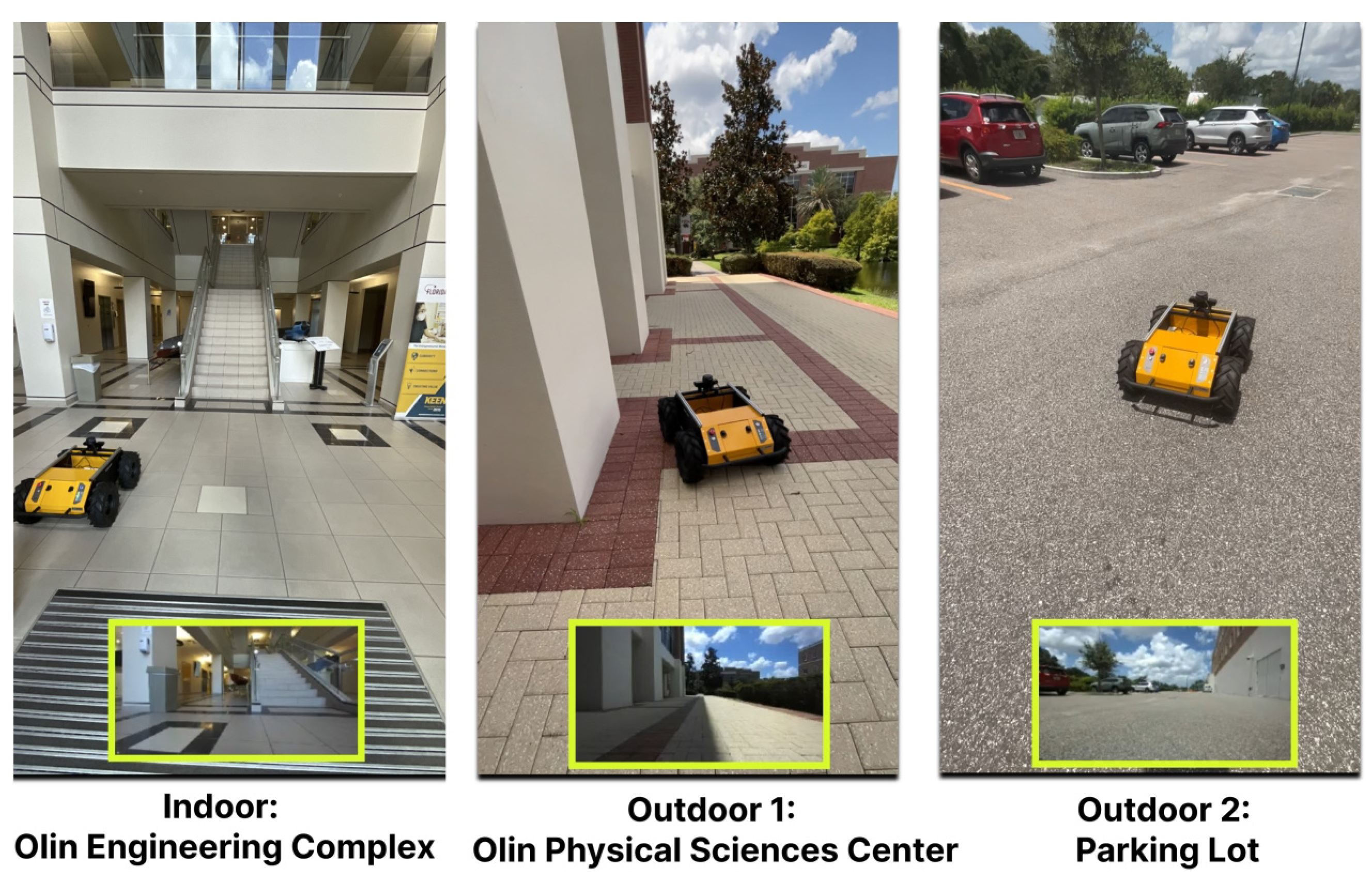
Experiments in real-world environments, including the indoor building (15 m × 15 m office with furniture), the outdoor front of the building (20 m × 20 m area with trees and pedestrians), and the parking lot (25 m × 25 m with cars and vehicles).
Figure 6.
Experiments in real-world environments, including the indoor building (15 m × 15 m office with furniture), the outdoor front of the building (20 m × 20 m area with trees and pedestrians), and the parking lot (25 m × 25 m with cars and vehicles).
Figure 7.
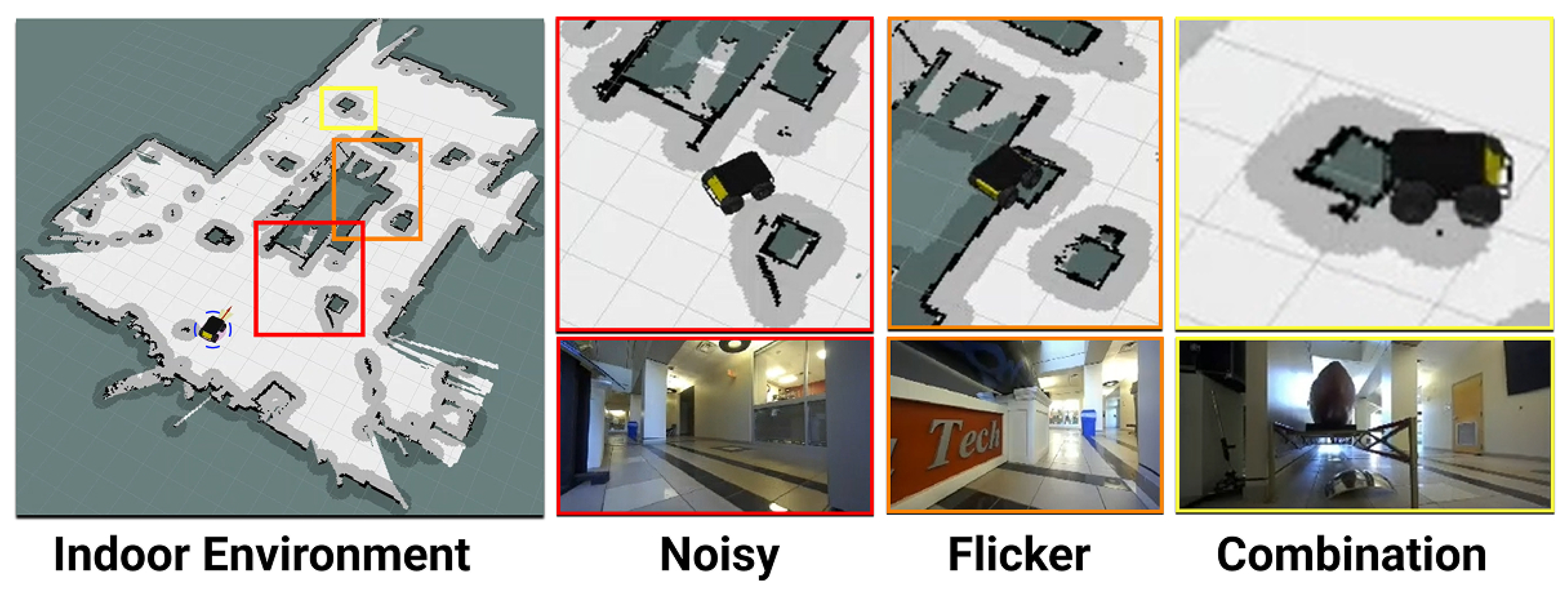
Partial observability effects on AMCL (a traditional method) in the indoor environment. The left image shows the pre-mapped 2D map with a blue circle marking the robot’s starting position. The right three columns depict the following: (1) noise causing navigation failure through a narrow path due to the robot perceiving obstacles as closer, (2) sensor flickering misaligning the robot’s map position into the stairs obstacle, and (3) their combination resulting in collisions with a shifted position. The red arrow indicates the direction that the Husky is facing.
Figure 7.
Partial observability effects on AMCL (a traditional method) in the indoor environment. The left image shows the pre-mapped 2D map with a blue circle marking the robot’s starting position. The right three columns depict the following: (1) noise causing navigation failure through a narrow path due to the robot perceiving obstacles as closer, (2) sensor flickering misaligning the robot’s map position into the stairs obstacle, and (3) their combination resulting in collisions with a shifted position. The red arrow indicates the direction that the Husky is facing.
Figure 8.
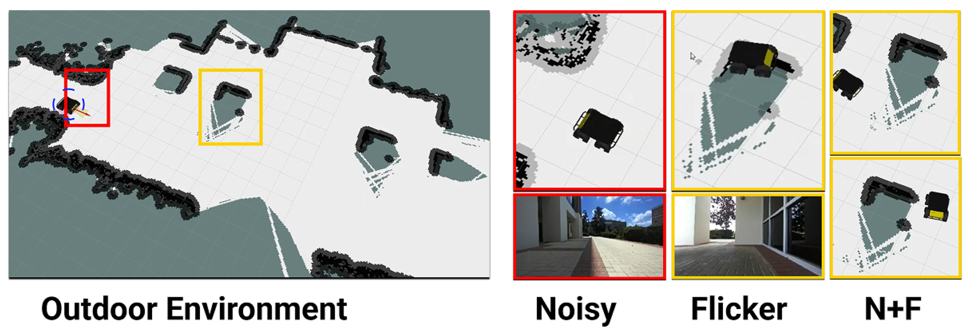
Partial observability effects on AMCL (a traditional method) in an outdoor environment. The left image shows the pre-mapped 2D map with a blue circle marking the robot’s starting position. The right three columns each display a zoomed region of the map where the robot failed to navigate, paired with the robot’s corresponding point of view, depicting the following: (1) noise causing the robot to stop moving after advancing despite distant obstacles due to excessive range uncertainty triggering a safety stop or perceived self-collision, (2) sensor flickering shifting the robot’s map position into the pillar obstacle, and (3) their combination resulting in a longer path to the destination. The red arrow indicates the direction that the Husky is facing.
Figure 8.
Partial observability effects on AMCL (a traditional method) in an outdoor environment. The left image shows the pre-mapped 2D map with a blue circle marking the robot’s starting position. The right three columns each display a zoomed region of the map where the robot failed to navigate, paired with the robot’s corresponding point of view, depicting the following: (1) noise causing the robot to stop moving after advancing despite distant obstacles due to excessive range uncertainty triggering a safety stop or perceived self-collision, (2) sensor flickering shifting the robot’s map position into the pillar obstacle, and (3) their combination resulting in a longer path to the destination. The red arrow indicates the direction that the Husky is facing.
Figure 9.
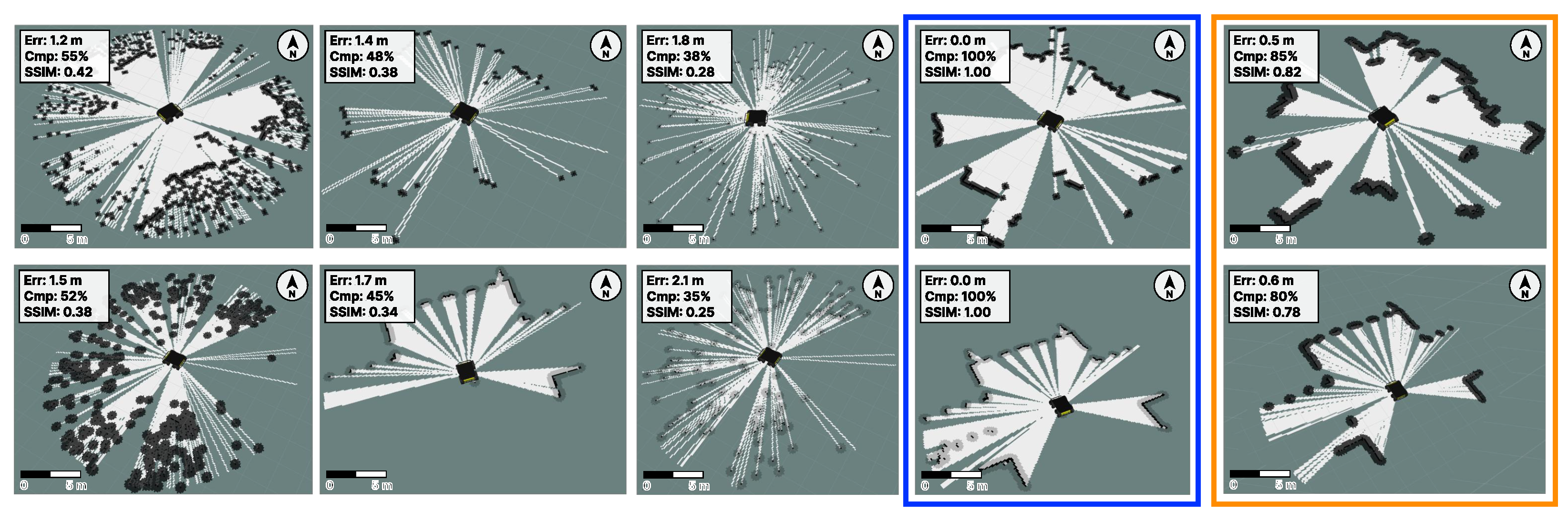
Effect of noise, flickering, and their combination on Gmapping maps (first three columns). Rows represent indoor and outdoor environments. Columns show noise, flickering, combination, ground-truth, and QSNE results, highlighting improved map accuracy with the QSNE framework. The black dots represent raw sensor data points captured by the robot’s lidar. These dots indicate detected obstacles or surfaces within the robot’s field of view. Each panel carries three on-figure annotations: a 5 m scale bar in the lower-left corner; a north-arrow marker in the upper-right corner; and a metric overlay in the upper-left corner that reports the map error (Err, in meters), the map completeness (Cmp, in percent), and the structural similarity index (SSIM) against the ground-truth map of the matching row. Blue and orange boxes show the ground-truth and QSNE results.
Figure 9.
Effect of noise, flickering, and their combination on Gmapping maps (first three columns). Rows represent indoor and outdoor environments. Columns show noise, flickering, combination, ground-truth, and QSNE results, highlighting improved map accuracy with the QSNE framework. The black dots represent raw sensor data points captured by the robot’s lidar. These dots indicate detected obstacles or surfaces within the robot’s field of view. Each panel carries three on-figure annotations: a 5 m scale bar in the lower-left corner; a north-arrow marker in the upper-right corner; and a metric overlay in the upper-left corner that reports the map error (Err, in meters), the map completeness (Cmp, in percent), and the structural similarity index (SSIM) against the ground-truth map of the matching row. Blue and orange boxes show the ground-truth and QSNE results.
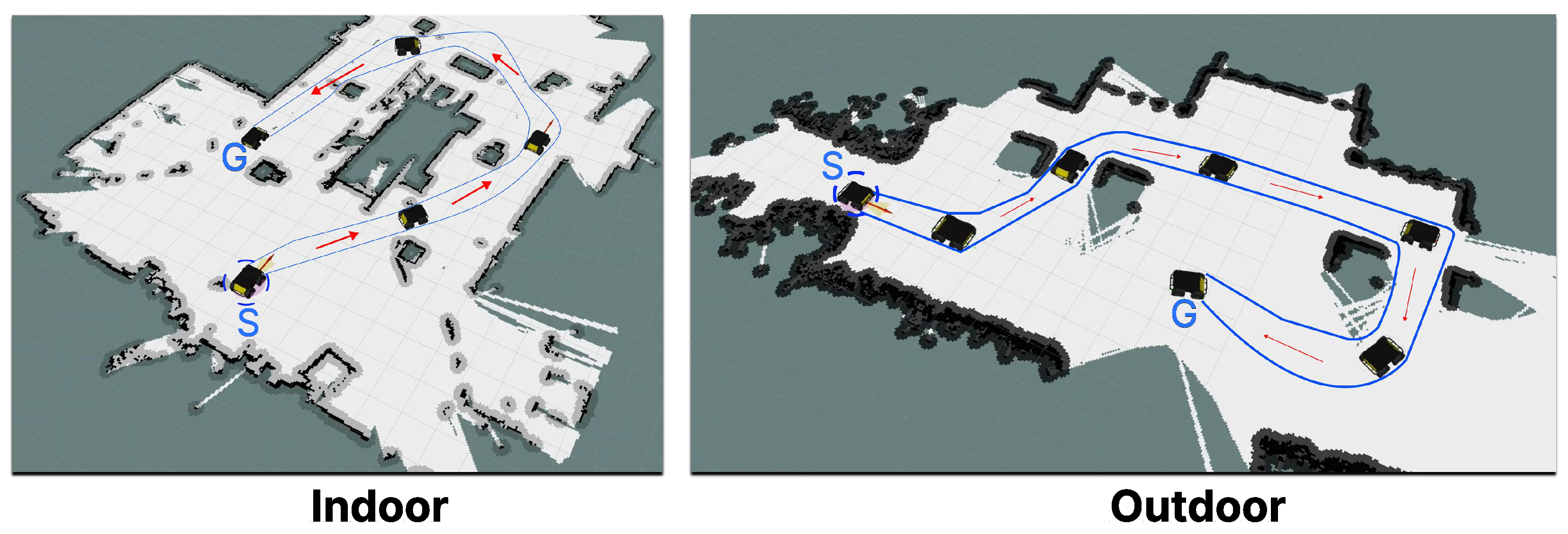
Figure 10.
Navigation paths of the Husky UGV using the proposed QSNE framework under partial observability. In each panel, a blue character labeled ‘S’ marks the start position and ‘G’ marks the goal. The (left) image shows the indoor environment with a blue starting circle and a blue path with red arrows. The red arrow indicates the direction that the Husky is facing. The (right) image displays the outdoor environment with similar markings.
Figure 10.
Navigation paths of the Husky UGV using the proposed QSNE framework under partial observability. In each panel, a blue character labeled ‘S’ marks the start position and ‘G’ marks the goal. The (left) image shows the indoor environment with a blue starting circle and a blue path with red arrows. The red arrow indicates the direction that the Husky is facing. The (right) image displays the outdoor environment with similar markings.
Figure 11.
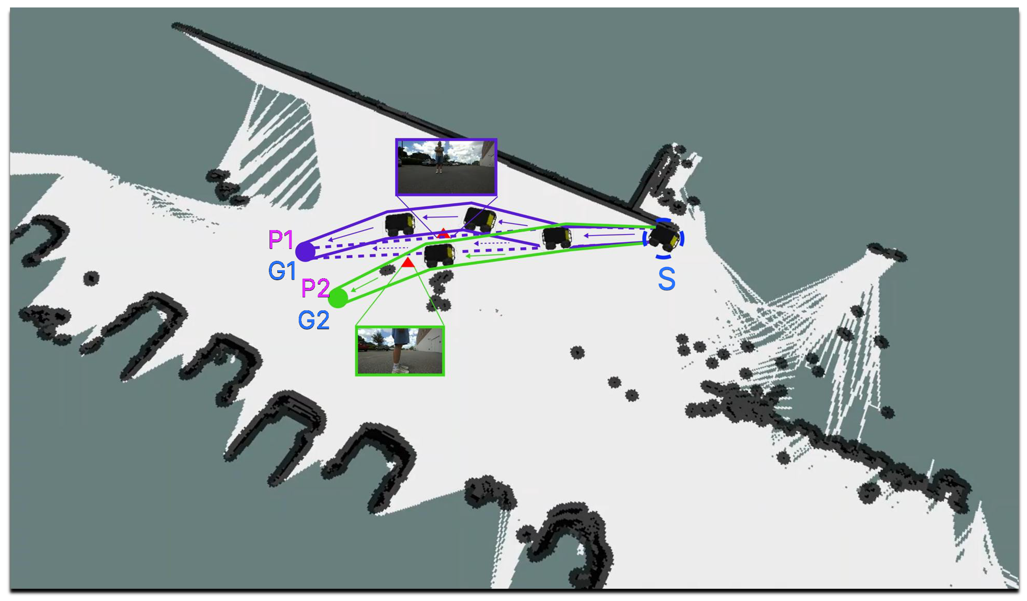
Navigation paths in the dynamic parking lot with human intervention. A blue character labeled ‘S’ marks the start position, and ‘G’ marks the goal. The image shows the robot’s starting position (blue circle), paths from P1 and P2, and inset views of human obstacles. P1 illustrates a right shift at 1.5 m, while P2 shows a stop at 2 feet. The red triangles show the pedestrian positions. The dashed purple line is the planned path to P1; the solid purple arrows trace the actual path, which detours around the first pedestrian after detection. The solid green arrows trace the path toward P2 and terminate where a second pedestrian stepped into the lane at close range and prompted a full stop. The purple and green photo insets show the on-board camera view of each pedestrian.
Figure 11.
Navigation paths in the dynamic parking lot with human intervention. A blue character labeled ‘S’ marks the start position, and ‘G’ marks the goal. The image shows the robot’s starting position (blue circle), paths from P1 and P2, and inset views of human obstacles. P1 illustrates a right shift at 1.5 m, while P2 shows a stop at 2 feet. The red triangles show the pedestrian positions. The dashed purple line is the planned path to P1; the solid purple arrows trace the actual path, which detours around the first pedestrian after detection. The solid green arrows trace the path toward P2 and terminate where a second pedestrian stepped into the lane at close range and prompted a full stop. The purple and green photo insets show the on-board camera view of each pedestrian.
Figure 12.
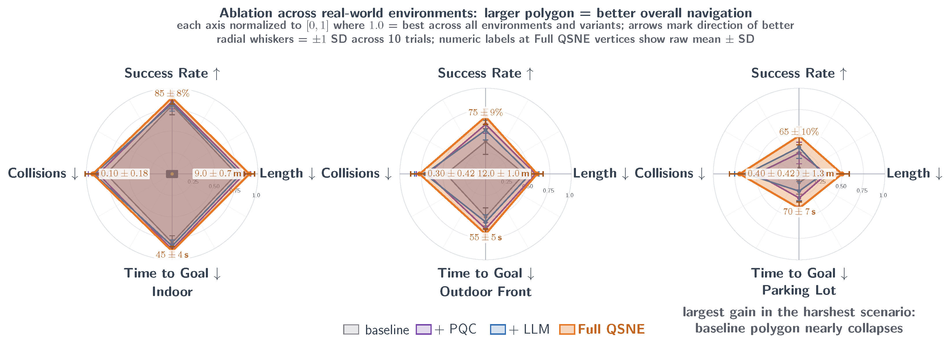
Real-world ablation, drawn as polar plots with one panel per environment and four metric axes per panel. Each axis is normalized to , where is the best value observed across all environments and variants; lower-is-better metrics are inverted, so a larger polygon indicates better overall navigation. Full QSNE (orange) encloses the other variants in every environment. The gap is largest in the Parking Lot, where the ordinary PPO-LSTM polygon contracts to near the centre. Means over 10 trials per environment under 50% Gaussian noise (std m) and 50% ray dropout. The ↑ on Success Rate marks higher-is-better; the ↓ on Length, Time to Goal, and Collisions marks lower-is-better. All four axes are normalized to , so a larger polygon area indicates a better overall result on every metric.
Figure 12.
Real-world ablation, drawn as polar plots with one panel per environment and four metric axes per panel. Each axis is normalized to , where is the best value observed across all environments and variants; lower-is-better metrics are inverted, so a larger polygon indicates better overall navigation. Full QSNE (orange) encloses the other variants in every environment. The gap is largest in the Parking Lot, where the ordinary PPO-LSTM polygon contracts to near the centre. Means over 10 trials per environment under 50% Gaussian noise (std m) and 50% ray dropout. The ↑ on Success Rate marks higher-is-better; the ↓ on Length, Time to Goal, and Collisions marks lower-is-better. All four axes are normalized to , so a larger polygon area indicates a better overall result on every metric.
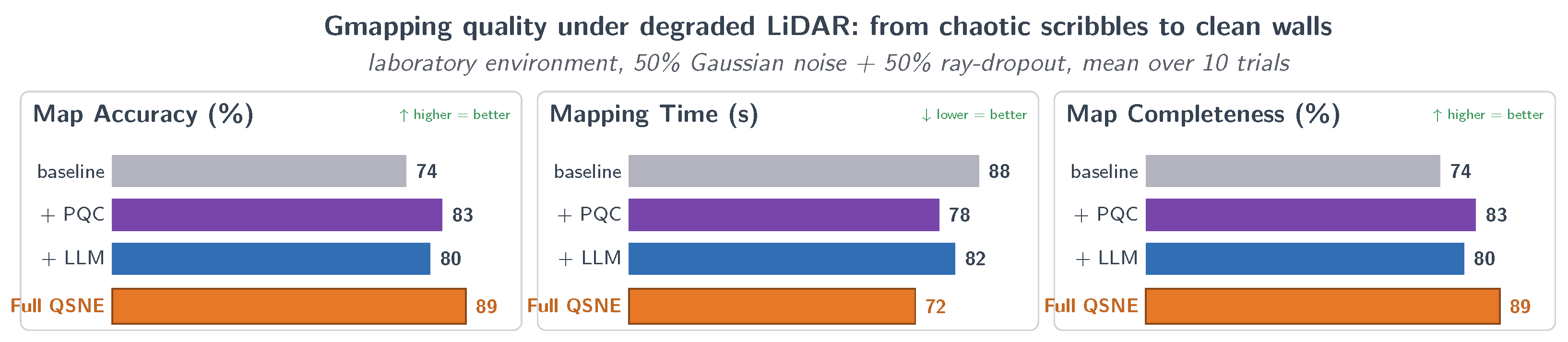
Figure 13.
Gmapping reconstruction quality in the laboratory environment under 50% Gaussian noise and 50% ray dropout (mean over 10 trials). The three panels report map accuracy, mapping time, and map completeness for the four ablation variants. The full QSNE achieves 89% map accuracy and 89% completeness with a mapping time of 72 s, the best result on every metric. The per-component decomposition of the result is reported in
Table 7.
Figure 13.
Gmapping reconstruction quality in the laboratory environment under 50% Gaussian noise and 50% ray dropout (mean over 10 trials). The three panels report map accuracy, mapping time, and map completeness for the four ablation variants. The full QSNE achieves 89% map accuracy and 89% completeness with a mapping time of 72 s, the best result on every metric. The per-component decomposition of the result is reported in
Table 7.
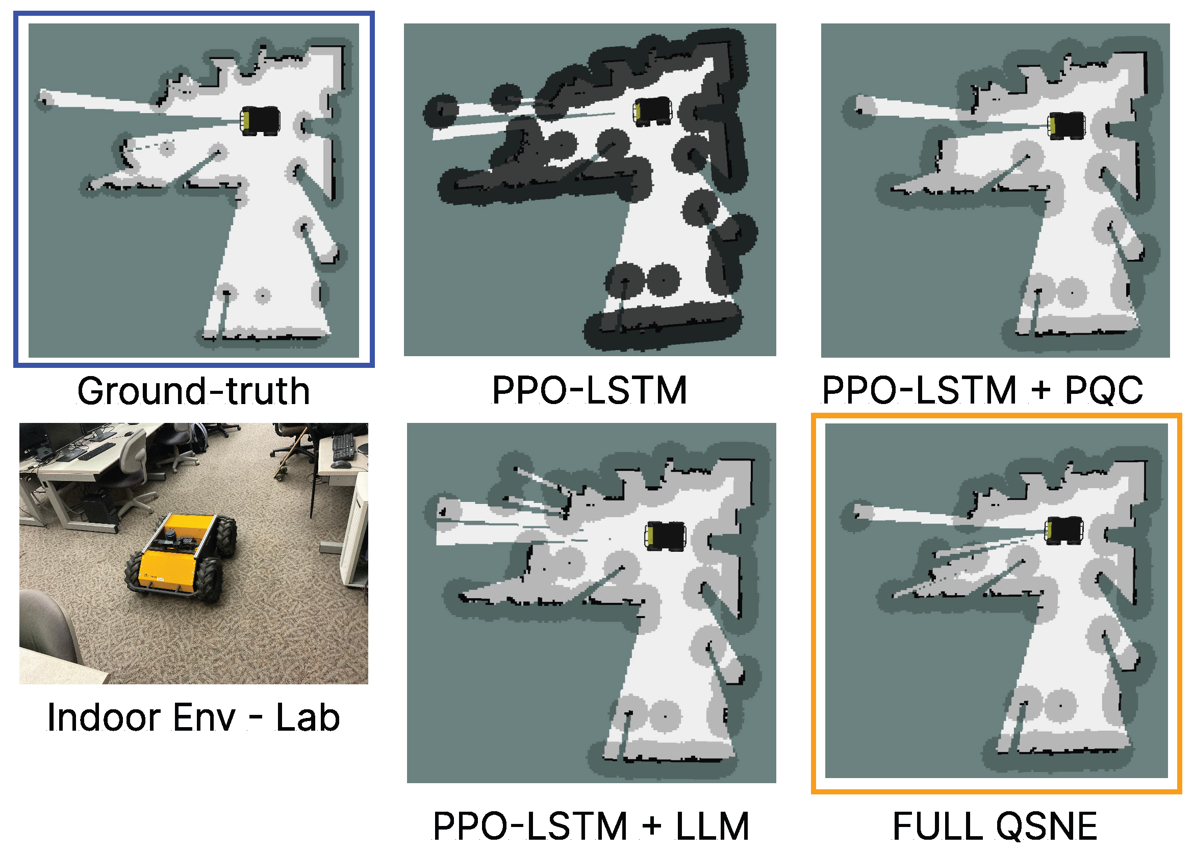
Figure 14.
Comparison of generated maps in the indoor laboratory environment. The ground-truth map (top-left, blue border) serves as reference. The real lab environment with the Husky UGV appears in the bottom-left. Maps from the four ablation variants demonstrate progressive improvement. The full QSNE (bottom-right, orange border) achieves the highest fidelity to the ground-truth.
Figure 14.
Comparison of generated maps in the indoor laboratory environment. The ground-truth map (top-left, blue border) serves as reference. The real lab environment with the Husky UGV appears in the bottom-left. Maps from the four ablation variants demonstrate progressive improvement. The full QSNE (bottom-right, orange border) achieves the highest fidelity to the ground-truth.
Table 1.
Per-component inference time, hardware location, and real-time impact of each module in the QSNE pipeline. Frequencies are expressed relative to the 10 Hz control loop. The LLM call is the only component that runs off-board, and the asynchronous ROS architecture prevents it from blocking the control loop. The LLM latency in this table is the mean ± standard deviation over 1000 deployment calls collected across the full real-world scenario.
Table 1.
Per-component inference time, hardware location, and real-time impact of each module in the QSNE pipeline. Frequencies are expressed relative to the 10 Hz control loop. The LLM call is the only component that runs off-board, and the asynchronous ROS architecture prevents it from blocking the control loop. The LLM latency in this table is the mean ± standard deviation over 1000 deployment calls collected across the full real-world scenario.
| Component | Hardware | Inference Time | Call Frequency | Blocks Control Loop? |
|---|
| PPO-LSTM policy + value head | Onboard CPU (i7-12700H) | ms | Every step (10 Hz) | Yes (within 100 ms budget) |
| Scan-reconstruction decoder | Onboard CPU | ms | Every step (10 Hz) | Yes (within 100 ms budget) |
| PQC (6 qubits, 4 layers) | Onboard CPU (PennyLane) | ms | Every step (10 Hz) | Yes (within 100 ms budget) |
| Transformer encoder (DistilBERT) | Onboard CPU | ms | Per LLM response (≈1.3 Hz) | No (asynchronous node) |
| GPT-4o API call | Cloud (OpenAI, campus Wi-Fi) | ms | Once per 10 steps or on | No (asynchronous node) |
| Total on-board per step | Onboard CPU | ms | Every step (10 Hz) | 19.4 ms of 100 ms budget |
Table 2.
End-to-end latency profile of the semantic-reasoning module, reported as median and 95th-percentile (
) over 500 controlled indoor profiling calls with the hosted GPT-4o API. This corresponds to a per-stage breakdown of the LLM latency in
Table 1, which reports the mean ± standard deviation over the full 1000-call deployment campaign. The aggregate latency exceeds the 100 ms control-loop budget by roughly a factor of six and motivates the asynchronous execution mode described in
Section 2.4.
Table 2.
End-to-end latency profile of the semantic-reasoning module, reported as median and 95th-percentile (
) over 500 controlled indoor profiling calls with the hosted GPT-4o API. This corresponds to a per-stage breakdown of the LLM latency in
Table 1, which reports the mean ± standard deviation over the full 1000-call deployment campaign. The aggregate latency exceeds the 100 ms control-loop budget by roughly a factor of six and motivates the asynchronous execution mode described in
Section 2.4.
| Component | Median (ms) | (ms) | Share of Median (%) |
|---|
| Prompt assembly | 1.8 | 2.6 | 0.3 |
| GPT-4o round trip | 612 | 1410 | 98.9 |
| Response parsing | 0.9 | 1.4 | 0.1 |
| Transformer encoding () | 4.2 | 6.1 | 0.7 |
| Total | 619 | 1420 | 100.0 |
Table 3.
QSNE hyperparameters. The table is grouped in four blocks: PPO training, LSTM and policy/value heads, PQC, and LLM and semantic reasoning. Values were either taken from the original references or selected via the sensitivity sweeps reported in
Section 3.3.
Table 3.
QSNE hyperparameters. The table is grouped in four blocks: PPO training, LSTM and policy/value heads, PQC, and LLM and semantic reasoning. Values were either taken from the original references or selected via the sensitivity sweeps reported in
Section 3.3.
| Block | Hyperparameter (Symbol) | Value | Rationale/Source |
|---|
| PPO training | Total time steps | | Convergence point in training progress |
| Learning rate | | Standard PPO default |
| Batch size | 64 | Standard PPO default |
| Entropy coefficient | | Encourages exploration under degradation |
| Clip parameter () | | Schulman et al. PPO recommendation |
| Discount factor () | | Standard long-horizon value |
| GAE | | Standard PPO default |
| LSTM + heads | LSTM hidden units | 128 | Capacity sufficient for 720-ray temporal context |
| Policy/value FC layers | | Matches Stable Baselines3 default |
| Action space (clipped) | m/s, rad/s | Husky UGV velocity limits |
| Initial action std () | | Tuned empirically |
| PQC | Number of qubits | 6 | Selected via PQC qubit-count |
| Number of variational layers | 4 | Selected via PQC depth |
| Rotation gates | | Angle-encoding standard |
| Entangling gates | CNOT (linear chain) | Nearest-neighbor entanglement |
| Measurement basis | Pauli-Z per qubit | Yields |
| LLM + reasoning | Backbone | GPT-4o | Hosted API |
| Sector count | 12 | 30° per sector, balances detail vs. prompt size |
| Embedding dimension () | 256 | Transformer encoder output |
| Query interval (steps) | 10 | Balances responsiveness and API cost |
| Variance trigger threshold () | | Matches noise std; triggers reasoning under uncertainty |
| Model snapshot | gpt-4o-2024-08-06 | Frozen version pin; no fine-tuning |
| Execution mode | Asynchronous, background thread | Decouples 619 ms LLM RTT from 100 ms control budget |
Table 4.
Performance comparison for AMCL with and without the hybrid framework in real-world environments (10 trials each); values reported as mean ± standard deviation. The QSNE standard deviations are smaller than AMCL’s on every metric in every environment, which indicates a more stable system. The associated 95% confidence half-widths and the rationale for the 10-trial protocol are stated at the start of
Section 3.2.
Table 4.
Performance comparison for AMCL with and without the hybrid framework in real-world environments (10 trials each); values reported as mean ± standard deviation. The QSNE standard deviations are smaller than AMCL’s on every metric in every environment, which indicates a more stable system. The associated 95% confidence half-widths and the rationale for the 10-trial protocol are stated at the start of
Section 3.2.
| Environment | Success Rate (%) | Path Length (m) | Time to Goal (s) | Collisions/Trial |
|---|
| Indoor Environment (AMCL) | 80 ± 13 | 10.5 ± 1.4 | 50 ± 7 | 0.3 ± 0.5 |
| Indoor Env. (our method: QSNE) | 85 ± 8 | 9.0 ± 0.7 | 45 ± 4 | 0.1 ± 0.3 |
| Outdoor Front (AMCL) | 55 ± 15 | 13.5 ± 2.0 | 65 ± 10 | 0.7 ± 0.6 |
| Outdoor Front (QSNE) | 75 ± 9 | 12.0 ± 1.0 | 55 ± 5 | 0.3 ± 0.4 |
| Parking Lot (AMCL) | 20 ± 18 | 16.5 ± 2.9 | 85 ± 14 | 1.2 ± 0.9 |
| Parking Lot (QSNE) | 65 ± 10 | 13.0 ± 1.3 | 70 ± 7 | 0.4 ± 0.4 |
Table 5.
Performance comparison of QSNE versus Gmapping in real-world environments (10 trials each); values reported as mean ± standard deviation. The associated 95% confidence half-widths and the rationale for the 10-trial protocol are stated at the start of
Section 3.2.
Table 5.
Performance comparison of QSNE versus Gmapping in real-world environments (10 trials each); values reported as mean ± standard deviation. The associated 95% confidence half-widths and the rationale for the 10-trial protocol are stated at the start of
Section 3.2.
| Environment | Map Error (m) | Mapping Time (s) | Map Completeness (%) |
|---|
| Indoor Environment (Gmapping) | 0.8 ± 0.18 | 90 ± 12 | 70 ± 9 |
| Indoor Env. (QSNE) | 0.5 ± 0.09 | 75 ± 7 | 85 ± 5 |
| Outdoor Front (Gmapping) | 1.0 ± 0.25 | 100 ± 15 | 65 ± 11 |
| Outdoor Front (QSNE) | 0.6 ± 0.12 | 85 ± 8 | 80 ± 6 |
| Parking Lot (Gmapping) | 1.5 ± 0.42 | 120 ± 22 | 50 ± 14 |
| Parking Lot (QSNE) | 0.9 ± 0.18 | 95 ± 10 | 70 ± 7 |
Table 6.
Ablation results—Gazebo simulation worlds (mean ± standard deviation over 10 trials per world).
Table 6.
Ablation results—Gazebo simulation worlds (mean ± standard deviation over 10 trials per world).
| Environment | Variant | Success Rate (%) | Path Length (m) | Time to Goal (s) | Collisions/Trial |
|---|
| Inspection | PPO-LSTM | 65 ± 14 | 13.8 ± 1.7 | 78 ± 11 | 0.55 ± 0.42 |
| PPO-LSTM + PQC | 74 ± 11 | 12.1 ± 1.3 | 68 ± 8 | 0.32 ± 0.31 |
| PPO-LSTM + LLM | 71 ± 12 | 12.5 ± 1.4 | 72 ± 9 | 0.28 ± 0.28 |
| Full QSNE | 82 ± 8 | 10.9 ± 0.9 | 62 ± 6 | 0.15 ± 0.18 |
| Agriculture | PPO-LSTM | 82 ± 10 | 11.5 ± 1.2 | 64 ± 8 | 0.35 ± 0.30 |
| PPO-LSTM + PQC | 90 ± 7 | 10.2 ± 0.9 | 56 ± 6 | 0.20 ± 0.21 |
| PPO-LSTM + LLM | 87 ± 8 | 10.6 ± 1.0 | 59 ± 7 | 0.18 ± 0.19 |
| Full QSNE | 96 ± 5 | 9.4 ± 0.6 | 51 ± 4 | 0.10 ± 0.12 |
| Office | PPO-LSTM | 88 ± 8 | 9.8 ± 0.9 | 55 ± 6 | 0.25 ± 0.24 |
| PPO-LSTM + PQC | 93 ± 6 | 8.7 ± 0.7 | 48 ± 5 | 0.15 ± 0.16 |
| PPO-LSTM + LLM | 91 ± 7 | 9.1 ± 0.7 | 51 ± 5 | 0.12 ± 0.14 |
| Full QSNE | 98 ± 3 | 8.2 ± 0.5 | 45 ± 3 | 0.08 ± 0.10 |
| Construction | PPO-LSTM | 72 ± 13 | 13.1 ± 1.6 | 74 ± 10 | 0.52 ± 0.40 |
| PPO-LSTM + PQC | 80 ± 9 | 11.6 ± 1.2 | 65 ± 7 | 0.32 ± 0.28 |
| PPO-LSTM + LLM | 78 ± 10 | 12.0 ± 1.3 | 68 ± 8 | 0.28 ± 0.27 |
| Full QSNE | 88 ± 6 | 10.5 ± 0.8 | 58 ± 5 | 0.18 ± 0.20 |
Table 7.
Per-component contribution to the laboratory mapping experiment of
Figure 13. Marginal contribution is reported as the change relative to the PPO-LSTM baseline. Relative share is the marginal contribution expressed as a percentage of the total gain achieved by the full QSNE. The synergy row reports the difference between the full-QSNE gain and the arithmetic sum of the individual PQC and LLM marginal contributions; the near-zero values indicate that the two components combine in an approximately additive manner on these three map-quality metrics.
Table 7.
Per-component contribution to the laboratory mapping experiment of
Figure 13. Marginal contribution is reported as the change relative to the PPO-LSTM baseline. Relative share is the marginal contribution expressed as a percentage of the total gain achieved by the full QSNE. The synergy row reports the difference between the full-QSNE gain and the arithmetic sum of the individual PQC and LLM marginal contributions; the near-zero values indicate that the two components combine in an approximately additive manner on these three map-quality metrics.
| Variant/Contribution | Map Accuracy (%) | Acc (pp) | Mapping Time (s) | Time (s) | Completeness (%) | Comp (pp) |
|---|
| Baseline (PPO&LSTM) | 74 | — | 88 | — | 74 | — |
| +PQC (marginal) | 83 | +9 | 78 | −10 | 83 | +9 |
| +LLM (marginal) | 80 | +6 | 82 | −6 | 80 | +6 |
| Full QSNE (PPO&LSTM + PQC + LLM) | 89 | +15 | 72 | −16 | 89 | +15 |
| Relative share of full gain—PQC | — | 60% | — | 63% | — | 60% |
| Relative share of full gain—LLM | — | 40% | — | 37% | — | 40% |
| Synergy (full − PQC − LLM) | — | 0 | — | 0 | — | 0 |
Table 8.
PQC qubit-count sweep at fixed depth of four layers (PPO-LSTM + PQC variant, indoor real-world environment, 10 trials per configuration, mean ± standard deviation).
Table 8.
PQC qubit-count sweep at fixed depth of four layers (PPO-LSTM + PQC variant, indoor real-world environment, 10 trials per configuration, mean ± standard deviation).
| Qubits | Success Rate (%) | Path Length (m) | Training Time (min) | Inference Latency (ms) |
|---|
| 4 | 79 ± 10 | 9.6 ± 0.9 | 42 | 5.1 |
| 6 (default) | 83 ± 8 | 9.2 ± 0.7 | 52 | 7.1 |
| 8 | 84 ± 8 | 9.1 ± 0.7 | 68 | 9.8 |
Table 9.
PQC depth sweep at fixed width of six qubits (PPO-LSTM + PQC variant, indoor real-world environment, 10 trials per configuration, mean ± standard deviation). Four layers maximize success rate; deeper circuits show diminishing returns and substantially higher training cost.
Table 9.
PQC depth sweep at fixed width of six qubits (PPO-LSTM + PQC variant, indoor real-world environment, 10 trials per configuration, mean ± standard deviation). Four layers maximize success rate; deeper circuits show diminishing returns and substantially higher training cost.
| Layers | Success Rate (%) | Path Length (m) | Training Time (min) | Inference Latency (ms) |
|---|
| 2 | 78 ± 11 | 9.7 ± 0.9 | 38 | 4.6 |
| 4 (default) | 83 ± 8 | 9.2 ± 0.7 | 52 | 7.1 |
| 6 | 83 ± 9 | 9.2 ± 0.8 | 74 | 10.4 |