2. Related Work
The use of GMMs for monitoring industrial and chemical processes includes centralized [
4,
5,
6,
7,
8,
9] and distributed [
3,
10] solutions.
In the seminal work in [
4], the use of GMMs was introduced as an extension of the classic approach of principal component analysis. GMMs enable the monitoring of sensor data or observations that do not follow a normal distribution and of processes with multiple operating states. In [
5], a Bayesian inference strategy is used to compute the posterior probability of observations belonging to each Gaussian component, and a probability index is used to detect process faults around different operating regions. The problem of dynamic processes (i.e., updates of GMM parameter values) is addressed in [
6,
7,
8]. In [
6], particle-filtered Bayesian inference statistics are used to detect anomalies. In [
7], the problem is addressed by identifying the Gaussian component that needs to be updated and by updating its parameters with a moving window that selects the recent history of observations. In [
8], a Chernoff bound is used to determine the number of unfit observations needed to determine when the GMM is considered unfit. The problem of monitoring online batch processes is addressed in [
9]. In online monitoring, only observations up to the current time step are available, and they may not conform to the nominal distribution even if there are no anomalies.
The previous solutions require that all observations be processed in a single computing system, so these solutions are not distributed. This means that all observations need to be delivered to a single node if coming from sensors distributed over the industrial setting. Recent progress in monitoring with GMMs has transitioned to distributed solutions. In [
10], the centralized solution presented in [
5] is further developed to several local GMMs extracted from a global GMM and applied for distributed monitoring. This is achieved by grouping variables of the global GMM depending on the industrial unit they belong to (e.g., reactor, condenser, or workshop with coupled units) and deriving a GMM for each group. It is assumed that the process is in a faulty state if the observations in any local GMM are unfit. This distributed strategy is further developed in [
3] by grouping variables using canonical correlation analysis. Principal component analysis is also performed on a global basis to determine the contribution of each group to the industrial process, enabling online monitoring.
Other related distributed algorithms are presented in [
11,
12], but these consist of a single Gaussian component, not a mixture as in GMMs, or extensions of other classic techniques, including principal component analysis, canonical correlation analysis, and partial least-squares.
There is another body of work outside the context of industrial/chemical processes that addresses the problem of monitoring in distributed computer systems [
13,
14,
15,
16,
17,
18,
19]. Consider a function that depends on variables captured by sensors distributed in an area. The objective is to evaluate the function within a given accuracy level while minimizing data communication with a coordinator to reduce bandwidth and power consumption. The function in [
13] is a binary indicator of when the frequency of a single type of event exceeds a threshold value. A heuristic algorithm is proposed that sets local thresholds at each sensor and initiates communication with the coordinator only when the local frequency exceeds the local threshold. The function in [
14] is
, where
is the frequency of the
ith type of event and
p = 0, 1, or 2. Their contributions are upper and lower bounds on the communication complexity to evaluate the function within a given accuracy level. The function in [
15] is a global property of the network graph (e.g., network diameter) that is decomposed into local conditions that nodes can evaluate with data collected from their local neighborhood. The function in [
16] is arbitrary. Its evaluation is achieved with automatic differentiation and numerical optimization to derive local constraints, which are monitored with the geometric monitoring protocol, a proactive monitoring approach. The bandwidth consumption of geometric monitoring is addressed in [
17], and an application of the previous monitoring technique is [
18], where a coordinator is used to implement linear discriminant analysis on the data collected from the sensor network. On the other hand, a reactive monitoring protocol is proposed in [
19], in which a node issues a query that is flooded to all other nodes to evaluate local constraints. The coordinator is then elected to assess the responses.
GMMs have not been considered under the previous monitoring framework (i.e., in [
13,
14,
15,
16,
17,
18,
19]) to the best of our knowledge, and in the context of autonomous UAVs, the distributed approach considered in [
10] does not apply because it is not guaranteed that each UAV is assigned to a subset of Gaussian components due to their limited coverage. In other words, individual Gaussian components (i.e., individual target clusters) can be spread over a geographical area larger than the area covered by individual UAVs. The distributed approach considered in [
3] also does not apply because it assumes a large number of variables that correspond to individual sensors in the industrial plant. These variables are grouped according to the direction of transfer of energy throughout the industrial process, and methods are used to reduce dimensionality, given that the variables can be highly correlated. On the other hand, in the case of UAVs, only two variables are tracked: the
x and
y coordinates of the targets, and these variables do not correspond to the transfer of energy from
x to
y or vice versa.
It is also noted that, with the exception of [
19], all previous distributed algorithms [
3,
10,
11,
12,
13,
14,
15,
16,
17,
18] rely on a star topology where all nodes connect to a coordinator directly, and in [
19], a coordinator is elected dynamically to receive data from nodes via convergecast.
Table 1 classifies all monitoring algorithms.
The first contribution of this paper is an algorithm to monitor a function of global data (i.e., the negative log-likelihood defined in
Section 4). It compares the function with a threshold value to determine when the GMM is unfit. Our solution is inspired by the distributed algorithm presented in [
20] that uses GMMs for monitoring in peer-to-peer computer networks, so there is no coordinator as in [
3,
10,
11,
12,
13,
14,
15,
16,
17,
18,
19]. The concepts of
knowledge,
agreement, and
withheld knowledge are borrowed from [
20] to allow UAVs to communicate with neighboring UAVs iteratively until they can determine that the GMM is unfit. The intuition behind iterative data exchanges is to propagate knowledge that is local to each UAV across the FANET.
The second contribution of this paper is a distributed expectation maximization (EM) algorithm that updates the values of the GMM parameters when the GMM is found to be unfit by the first algorithm. The reason for adopting an EM algorithm different from the one implemented in [
20] is that their algorithm depends on a tree-network topology that centralizes computations at the root of the tree (i.e., convergecast). On the other hand, our goal is to build a network that avoids single points of failure, so our distributed EM implementation is instead based on a token-ring protocol [
21] in our FANET. It is an adaptation of the solution presented in [
22], where nodes communicate sequentially over a token-ring network to complete the maximization step of the EM problem in a distributed way. In our algorithm, UAVs pass a token over the FANET, and when a UAV receives the token, it communicates with all of its one-hop neighbors, not just the next UAV in the ring, as in [
22]. In this way, we implement distributed average consensus using Metropolis–Hastings (MH) weights to complete the maximization step of the EM problem faster. MH weights were adopted in [
23] from the centralized MH sampling technique of Markov chain Monte Carlo methods [
24,
25,
26]. The reason for our adoption of MH weights is that they guarantee the convergence of distributed average consensus in time-varying communication graphs [
23,
27,
28]. This means that our UAV network can solve the EM problem when the sets of one-hop neighbors of UAVs change over time.
MH weights were also used in [
29] for a diffusion-based algorithm originally proposed in [
30], but convergence is faster on our token ring network, as demonstrated in our simulation results in
Section 6. Other symmetric weights determined in [
31] induce convergence faster than MH weights but are calculated by convex optimization, so they are not suitable for time-varying communication graphs, as the optimization problem needs to be solved when the sets of one-hop neighbors of UAVs change. Other distributed EM algorithms for estimating GMMs include [
32,
33,
34,
35,
36,
37,
38], but they do not consider time-varying communication graphs. They consider networks of static nodes to the best of our knowledge.
Therefore, this paper contributes two distributed algorithms for the problems of (1) monitoring ground targets using GMMs with the goal of detecting the unfitness of the GMM when target locations change and (2) updating the GMM to the new target locations. The aim is to complete these two tasks while reducing the number of message exchanges among UAVs to increase the Nyquist rate of observations that can be monitored. To the best of our knowledge, this monitoring problem has not been addressed when UAVs have only partial coverage of target clusters under a communication graph that can change over time. The algorithms are evaluated through simulation for linear flight formations of 3 to 16 UAVs and grid formations of 9 to 121 UAVs as the number of target clusters increases from 2 to 16 and from 2 to 9 in linear and grid formations, respectively. The simulation results demonstrate performance superior to related algorithms to the best of our knowledge.
3. System Model
Let
be a set of UAVs that communicate over a connected graph. The set of one-hop neighbors of
is denoted as
. Each UAV communicates only with its one-hop neighbors. There is a set of observations
that, without loss of generality, are two-dimensional as they correspond to geolocations of moving targets on the ground, i.e.,
for
. The target locations at any point in time follow the distribution of a GMM of
k Gaussian components. Therefore, the probability density function (pdf) of
is provided in (1), where
and
are the pdf and weight of the
sth Gaussian component;
is provided in (2), where
and
are the mean and covariance matrix of the
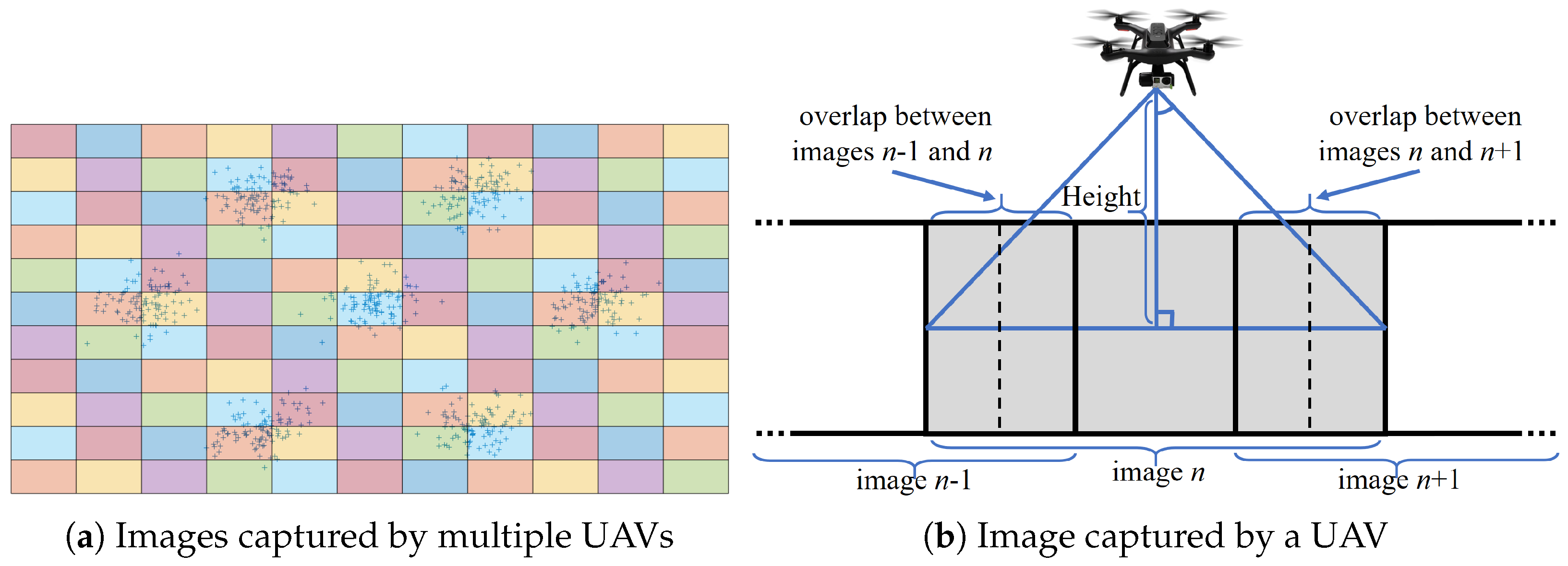
sth component. Each UAV captures images, as shown in
Figure 1b.
Figure 1a shows observations from a GMM of 7 components.
The area covered by UAVs is divided into a grid, as shown in
Figure 1a. Each rectangle corresponds to the area that a UAV covers while hovering in the center of the rectangle, as shown in
Figure 1b. We call this UAV location the
waypoint of the corresponding rectangle.
Figure 1b also shows that the adjacent images overlap. The UAV is capturing the
nth image in
Figure 1b. The images
and
are to the left and right of the
nth image, and this sequence of images can continue depending on the flight path of the UAV. This path is indicated with the dotted lines on images
and
. The overlap is purposely added to the flight paths due to errors in the location and orientation of the UAVs. Therefore, the images need to be realigned to form the grid in
Figure 1a. The problem of aligning images and locating targets in overlapping areas is beyond the scope of this paper. We address this problem in our previous work in [
39]. Each UAV is assigned a flight path that corresponds to a subset of waypoints on the grid and the order in which they are visited. UAVs fly through their sequence of waypoints periodically. We refer to a period as a
tour. Tours from different UAVs are assumed to be disjoint, which means that each waypoint is assigned to one and only one UAV. The set of observations detected by
during a tour is
.
It is assumed that UAVs cover all targets after the completion of all tours, i.e., . The observation sets of UAVs are disjointed, i.e., for all , because the tours are disjointed. It is also assumed that each UAV can communicate with one or more UAVs at one or more waypoints of the tour. The UAVs with which can communicate during a tour are ’s one-hop neighbors, i.e., .
UAVs are initialized with a priori values of
,
, and
. Therefore, it is assumed that the UAVs have already scanned the area in advance, as in [
40,
41], and the number of Gaussian components of the GMM has already been determined, as in [
42,
43]. Scanning unexplored areas is beyond the scope of this paper. The purpose of the periodic tours of this paper is to monitor the moving targets. It is also assumed that targets take more than one tour to move enough that the GMM parameters,
,
, and
, no longer correspond to the new target locations. The objective of this paper is two-fold. First, UAVs complete one or more tours to detect when the GMM parameters no longer correspond to the new target locations. We say that the GMM is unfit at this point. Second, UAVs calculate new parameter values to update the GMM.
It is also assumed that our algorithms are based on data-link protocols for wireless networks that detect packet losses and retransmit packets in response to the losses. Our monitoring algorithm then relies on data link acknowledgments to ensure that packets of each UAV are delivered to its one-hop neighbors. For example, our open-source UAV network [
1] implements UAV-to-UAV communication over a Zigbee network, which is based on the IEEE 802.15.4 protocol architecture. Our algorithm for updating the values of the GMM parameters is based on the wireless token ring protocol [
21], which we also implement over the Zigbee network.
4. Distributed Monitoring Algorithm
The objective of the monitoring algorithm is to determine whether , , and produce a GMM that does not fit the observations of the last tour of the UAVs. Unfitness of the GMM is defined as follows.
Definition 1. Let Θ be the set of GMM parameters, i.e., . Consider the negative log-likelihood of Θ given in (3), where is the number of observations in , i.e., . The average negative log-likelihood is defined as .
Definition 2. The GMM is classified as unfit when , where is provided in Definition 1, and ϵ is a threshold value defined by the user.
Let be one of ’s one-hop neighbors, i.e., . When they communicate, the message sent by to is , and it is a subset of the target locations from . Definitions 3 to 5 and Theorem 1 are used to determine the unfitness of the GMM in a distributed manner.
Definition 3. The knowledge of is .
Definition 4. The agreement of with is .
Definition 5. The withheld knowledge of from is .
The union operations in Definitions 3 and 4 do not differentiate observations of the same value, i.e., if , , and , then . Therefore, several observations of the same value are considered as one single observation. The reason is that two or more objects on the ground cannot occupy the same space, so target locations of the same value correspond to a single object on the ground.
The monitoring algorithm performs several message exchanges among UAVs. Therefore, the knowledge of a UAV propagates to other UAVs as the number of message exchanges increases. For example, consider three UAVs: , , and . Let their initial knowledge be , , and . Let and be within communication range of each other. Let and be within range of each other, too; and are not within range of each other. Their initial withheld knowledge is their full knowledge as they have not exchanged any messages yet, i.e., , , and . Now, let send a subset of observations from to . Let this subset be . Similarly, let the message from to be . Therefore, the agreement is . The knowledge and withheld knowledge of are updated after the messages are exchanged: and . The knowledge and withheld knowledge of are also updated: and . Now, let and exchange the following messages: and . Their knowledge and withheld knowledge are updated to the following values: , , , and . Therefore, a subset of the knowledge of reaches ; now knows of .
The next theorem is used to determine the required number of message exchanges that allow individual UAVs to calculate the unfitness of the GMM.
Theorem 1. if for , (1) , (2) , and either or for all .
Proof. Without loss of generalization, consider UAVs selected in some sequence , , …, and such that and are one-hop neighbors. Let all UAVs meet both conditions (1) and (2). When is selected, it sends to . Therefore, when is selected first, the new knowledge of becomes . Given that observations of the same value are considered as one single observation, the average negative log-likelihood of the new knowledge is , where . Therefore, given that and . Continuing this process, the new knowledge of is , and . □
Monitoring is implemented with two algorithms, one for transmission (Algorithm 1) and one for reception (Algorithm 2). UAVs self-select to transmit to their one-hop neighbors when they are within range during their tours. Self-selection can be implemented via periodic transmission of hello packets that allow UAVs to detect each other. Algorithm 1 takes place in each self-selection of . The outputs of the algorithm (line 2) are the messages sent to each neighbor in that is within range and a binary flag that signal the unfitness of the GMM parameters, i.e., . The inputs of the algorithm (line 1) are , the set of one-hop neighbors , ’s knowledge , its agreement with every neighbor , its knowledge withheld from every neighbor , and the number of transmissions T needed before testing unfitness of . The first step is to apply an indicator function that determines whether its argument is greater than . For example, indicates whether the average negative log-likelihood of knowledge is greater than (line 6). The message needs to be calculated and transmitted when is empty (line 9). The message also needs to be calculated and transmitted when does not match either or according to Theorem 1. These quantities are denoted by , , and (lines 6 to 8). The reason is calculated and transmitted when or is that these conditions indicate that and are not in agreement on the fitness of . Under either of these two conditions, the UAVs need to exchange withheld knowledge to reach an agreement. is assigned a subset of observations from (line 10). This subset is determined by selecting observations from until both and match . After is determined, the agreement and withheld knowledge are updated with (lines 11 and 12) because the observations in will now be known by after the transmission of (line 13).
Algorithm 1 keeps count of the number of self-selections since initialization with variable
t (line 16). If this number exceeds the threshold value
T, the algorithm determines if
is unfit (line 18). The value of
T needs to be high enough to allow all UAV knowledge to reach other UAVs that are a number of hops away. In this way, when
, UAVs can reliably determine the fitness of
. This is carried out by evaluating conditions (1) and (2) of Theorem 1 (lines 20 and 24). The flag defaults to
false (line 17), and if any of the conditions are not met, the flag becomes
true (lines 21 and 25), indicating that
is unfit. It should be noted that the event that any of conditions (1) and (2) is not met does not necessarily imply that
. There can be false alarms declaring
unfit. The false alarm rate can be decreased by increasing
T; however, increasing
T increases the time to determine unfitness of
.
Section 6.1 evaluates the number of self-selections (i.e.,
T) that are needed to reliably determine the flag value. This value is highly dependent on the diameter of the FANET, as demonstrated by the simulation results in
Section 6.1.
Algorithm 2 processes when receives the message from . The inputs are the message , the knowledge , and the agreement (line 1). There are no outputs. The sole purpose of the algorithm is to update ’s knowledge of and its agreement with (lines 5 and 6). The initialization is the same as the initialization of Algorithm 1.
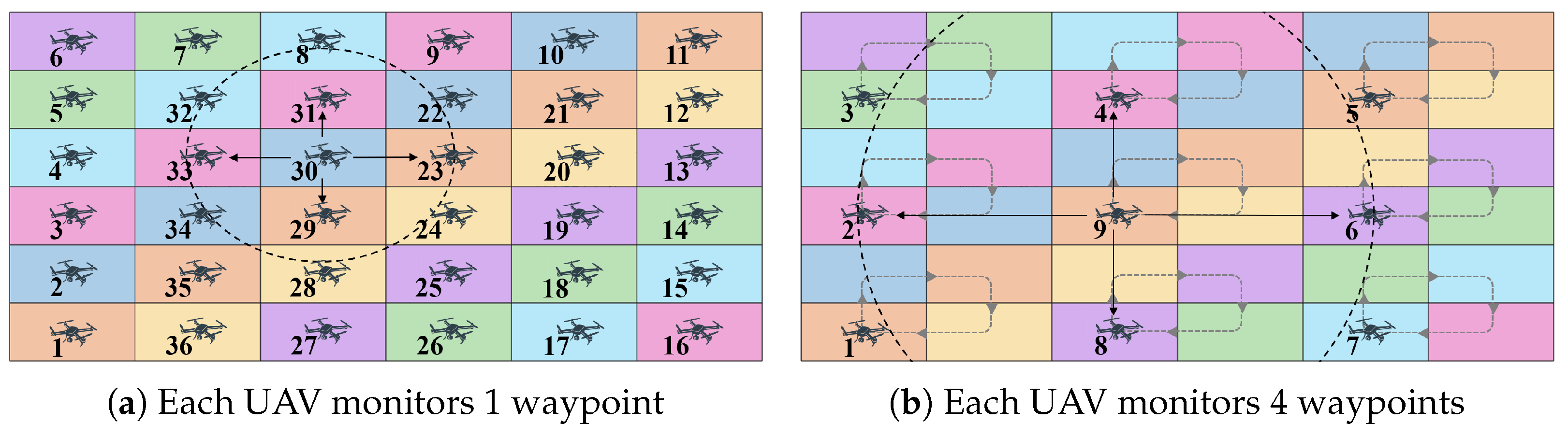
Figure 2 shows an example of the transmission in line 13 of Algorithm 1. In
Figure 2a,
is self-selected and transmits
,
,
, and
to its neighbors:
,
,
, and
. These transmissions take place one at a time. Each transmission corresponds to one loop of the
for loops in lines 5 to 15 of Algorithm 1. Each neighbor executes Algorithm 2 when it receives its corresponding message
. In
Figure 2b, each UAV monitors four waypoints. In this case,
has self-selected, and its transmission range is larger to reach its neighbors:
,
,
, and
.
| Algorithm 1 Monitoring Algorithm (Transmission) |
- 1:
Inputs: - 2:
Outputs: , f - 3:
Initialization: , , , - 4:
- 5:
for all do - 6:
- 7:
- 8:
- 9:
if or or do - 10:
- 11:
- 12:
- 13:
- 14:
end if - 15:
end for - 16:
- 17:
false - 18:
if
do - 19:
- 20:
if do - 21:
true - 22:
end if - 23:
for all do - 24:
if or do - 25:
true - 26:
end if - 27:
end for - 28:
end if
|
| Algorithm 2 Monitoring Algorithm (Reception). |
- 1:
Inputs: - 2:
Outputs: none - 3:
Initialization: same as Algorithm 1 - 4:
- 5:
- 6:
|
A UAV sends a message to each of its neighbors when it self-selects and executes Algorithm 1 (lines 5 to 15). It also evaluates its flag value after it has self-selected
T times (lines 17 to 28). However, evaluating the flag value does not require any communication with neighbors. Therefore, the communication complexity of the algorithm is determined by the number of neighbors (lines 5 to 15), and this number depends on the network topology. For example, UAVs have a maximum of four neighbors in the topology of
Figure 2. There are more topologies, with each having its own average and maximum number of neighbors. For example, when the topology is a random geometric graph (RGG), the average number of neighbors increases at a rate of
, where
is the number of UAVs, to ensure that the network is connected with high probability [
44]. Therefore, the communication complexity of Algorithm 1 is
in RGGs. The critical neighbor number of other topologies, including dense, sparse, and mobile networks, is the subject of [
45].
5. Distributed GMM Estimation
When one or more UAVs determine that
is unfit, the flag is true in Algorithm 1, and the UAVs begin to calculate new values for
. This can be accomplished by flooding the flag on the UAV network [
46].
The calculation of the new values of
is via expectation maximization [
47]. The EM algorithm consists of the execution of two iterative steps. It determines a value of
that decreases the average negative log-likelihood
until a termination criterion is met. The criterion in this paper is
because
is considered unfit when the criterion is not met according to Definition 2. The steps are the following:
Expectation Step: Estimate the contribution of each observation:
Maximization Step: Update the parameters
The maximization step in (5)–(7) depends on the set of all observations in . However, observations are distributed among , , …, and . Therefore, the EM algorithm can also be formulated as follows, where is ’s ath observation.
The expectation step in (8) is local to
. It only depends on its observations, i.e.,
. However, the maximization step depends on observations of all drones, i.e.,
,
, …, and
. To allow a distributed implementation of this step, we first note that (9)–(11) correspond to averages across all UAVs of the following quantities:
for (9),
for (10), and
for (11). Therefore, we complete the maximization step via distributed average consensus (DAC) [
31].
5.1. Distributed Average Consensus
Let
be
and assigned to
at time
. The DAC problem is to compute the average
in every UAV using message exchanges with only one-hop neighbors. A well-known equation for this operation is in (12), where
, is the weight associated with the one-hop link between
and
. Note that
if
and
are not one-hop neighbors.
Since one-hop links are undirected,
, and
. The weight matrix
needs to satisfy the following properties where
is the all-ones vector:
The calculation in (12) needs to converge to the average
of the DAC problem for all UAVs (i.e., for
) as follows:
Weights that satisfy the constraints in (13) and the asymptotic average consensus in (14) always exist. In this paper, we use the
Metropolis–Hastings (MH) weights [
23]:
5.2. Distributed Maximization Step
The averages in (9)–(11) are computed using DAC. Let
and apply (12) to calculate the average number of local targets per UAV, i.e.,
. Therefore,
DAC is applied to calculate (9) by letting
. Therefore,
DAC is applied to calculate (10) by letting
. Therefore,
Similarly, let
, then
5.3. Distributed EM Algorithm
Algorithm 3 performs a number of iterations (line 5) to evaluate the expectation step in (8) and the distributed maximization step in (16)–(18) until the termination criterion is met, i.e.,
according to Definition 2. The inputs of the algorithm (line 1) are the current and unfit GMM parameters
, the set of local observations
, and the MH weights between
and its one-hop neighbors, i.e.,
. The output (line 2) is the new GMM parameters
that satisfy the termination criterion.
| Algorithm 3 Distributed EM. |
- 1:
Inputs: , , - 2:
Output: - 3:
Initialization: for and according to (8), , , , - 4:
- 5:
while termination is false do - 6:
for all do - 7:
evaluate according to (12) - 8:
end for - 9:
for all do - 10:
evaluate according to (12) - 11:
end for - 12:
for all do - 13:
evaluate according to (12) - 14:
end for - 15:
termination ← false - 16:
for all do - 17:
evaluate according to (12) - 18:
according to (16) - 19:
according to (17) - 20:
according to (18) - 21:
- 22:
evaluate according to (8) for all s, a - 23:
if termination is false do - 24:
termination - 25:
end if - 26:
end for - 27:
end while
|
Algorithm 3 calculates using DAC, as demonstrated in (16)–(18). Initialization (line 3) consists of calculating the initial average values , , , and . Given that these values depend on for and , the evaluation of this quantity using (8) is the first step of the initialization.
Algorithm 3 operates on a token-ring protocol. The implementation of this protocol on wireless networks such as FANETs is well known [
21]. For example, the ring in
Figure 2a is the UAV sequence
,
, …, and
. The ring closes when
transmits to
. The ring in
Figure 2b is
,
, …, and
, and it closes when
or
relays the token from
to
because
is not within
’s range.
In the first round of Algorithm 3 (line 6), each UAV updates the running average that eventually converges to according to (15). Similarly, in the following three rounds (lines 9, 12, and 16), each UAV updates the other running averages: , , and . The averages are updated by communicating with one-hope neighbors according to (12).
After all running averages are updated, the new values of the GMM parameters, i.e.,
,
, and
, are calculated (lines 18, 19, and 20). The convergence of
to
(line 18) is demonstrated as follows:
The convergence of to (line 19) and the convergence of to can be demonstrated in a similar way.
The last calculation in Algorithm 3 before evaluating the termination criteria is the expectation step in (8), i.e., the evaluation of for and using the updated values of the GMM parameters , , and . This calculation depends on data local to , so it does not require communication with ’s one-hop neighbors.
Evaluation of the termination criterion (line 24) requires the calculation of , which is equivalent to according to Definition 1. Therefore, the criterion is evaluated by having the UAVs pass the values of and along the token ring network. The value of the criterion is defaulted to false (line 15) to iterate through the expectation and distributed maximization steps (lines 6 to 26) until all UAVs evaluate the criterion as true.
For each while loop of Algorithm 3 (lines 5 to 27), there are four rounds of communication over the token-ring network, which correspond to the for loops that begin on lines 6, 9, 12, and 16. Each UAV communicates with its neighbors according to (12). Given that the length of the ring is , the communication complexity of Algorithm 3 is then when the network topology is RGG.
6. Performance Evaluation
The monitoring algorithms (i.e., Algorithms 1 and 2) and the distributed EM algorithm (i.e., Algorithm 3) were implemented in MATLAB (v. R2024b), and their performance was evaluated by simulation for two flight formations, linear and grid.
The linear flight formation is shown in
Figure 3. Without loss of generality, it is assumed that each rectangular area corresponds to a UAV hovering at the center of the rectangle, as shown in
Figure 2a. Therefore, there are five UAVs in
Figure 3a,b. This assumption is to consider the worst-case scenario with the highest number of UAVs to cover all rectangular areas. In this scenario, the global set of targets is distributed across the largest set of UAVs because no single UAV covers more than one rectangular area. The rectangular areas correspond to images captured with a camera with horizontal and vertical fields of view of 62° and 49°, respectively.
It is also assumed that only adjacent UAVs are within communication range of each other, as shown in
Figure 2. Therefore, the left and right UAVs in
Figure 3 each have one neighbor, and all other UAVs have two neighbors each. This is the worst-case scenario in terms of network connectivity, i.e., the number of one-hop neighbors of each UAV is the minimum that keeps the network graph connected. The number of communication exchanges among UAVs to propagate their withheld knowledge increases as the connectivity decreases.
Two different cluster configurations are considered,
centered and
uncentered. The cluster centroids are in the center of the rectangular areas in the centered configuration (
Figure 3a), and they are at the border between adjacent areas in the uncentered configuration (
Figure 3b). All clusters have 100 targets and covariance matrix
unless otherwise specified.
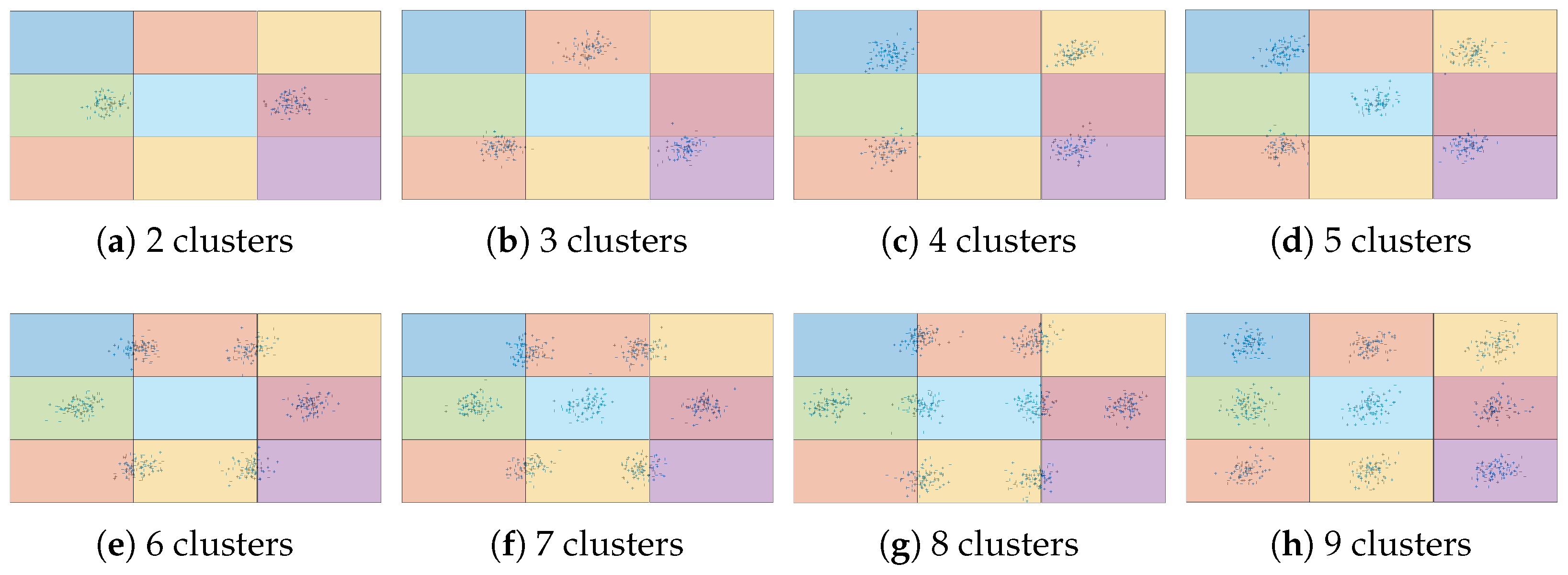
The grid flight formation is shown in
Figure 4. It is also assumed that each rectangular area corresponds to a hovering UAV in the center of the rectangle and that only adjacent UAVs are within communication range of each other, including both vertical and horizontal directions. Therefore, each of the UAVs at the corners of the grid has two neighbors; each of the other UAVs at the boundary of the grid has three neighbors, and each of the UAVs in the interior of the grid has four neighbors. There are eight different cluster configurations with an increasing number of clusters, starting with two clusters, as shown in
Figure 4a.
Figure 4b–h show the cluster configurations with three to nine clusters, respectively. The grids in
Figure 4 all have nine UAVs each, which is a grid of
. Larger grids are also included in our simulation results, from
to
. In these cases, rectangular areas decrease in size, and cluster configurations remain the same. For example,
Figure 1a shows the
grid with seven clusters, which are the same seven clusters shown in the
grid in
Figure 4f. Increasing the dimensions of the grid implies that the rectangular areas decrease in size to cover the same overall area. This is equivalent to covering the same overall area with a higher number of UAVs hovering at lower altitudes.
6.1. Performance Evaluation: Monitoring Algorithm
The performance of the monitoring algorithm is evaluated with the number of monitoring instances that UAVs need to perform until they all have the same flag value. We define a monitoring instance as the self-selection of a UAV to execute the transmission monitoring algorithm (Algorithm 1) and the corresponding execution of the monitoring algorithm for reception (Algorithm 2) at all UAVs that are within range. The number of monitoring instances corresponds to T in Algorithm 1. Therefore, if is unfit, we count the number of monitoring instances (MI) until all UAVs have a flag value of true, and if is a good fit, we count the number of MIs until all UAVs have a flag value of false. The number of MIs for all UAVs to acquire full knowledge is also evaluated. We say that a UAV acquires full knowledge when its knowledge (i.e., ) is equal to the global set of observations (i.e., ). The reason is that the centralized solution to the monitoring problem (i.e., determining if is unfit) requires knowledge of , but this information is not initially available in any single UAV but distributed across all UAVs (i.e., , , …, ).
The monitoring algorithm uses
. The value of
determines the average value of the joint pdf of the observations (i.e.,
for
) according to Definition 1. This means that the GMM is considered unfit when the average value of the joint pdf is less than
. We set its value at 3. Typical values for two-dimensional data range from 2 to 5. However, this value is application-dependent. It depends on the desired quality of the fit, variability of the data, and number of Gaussian components. The analysis of
is beyond the scope of this paper but is covered in depth in the GMM literature, including [
48].
6.1.1. Linear Formation
Figure 5 shows the number of MIs needed for all UAVs to acquire full knowledge and for all UAVs to determine that the GMM does not fit the observations (i.e., all UAVs’ flags become true). The number of MIs is plotted as a function of the number of UAVs in both cases, centered (
Figure 3a) and uncentered (
Figure 3b).
The number of MIs increases with the number of UAVs in all cases. However, the rate of increase is lower for the case that all flags become true. At 3 UAVs, the number of MIs for all flags to become true is 4 in both cases, centered and uncentered, and for full knowledge, it is 10 for both cases. On the other hand, at 15 UAVs, the number of MIs for all flags to become true is 30 for both cases, and the number of MIs for full knowledge is 245 and 264 for the centered and uncentered cases, respectively.
The higher rate of increase for full knowledge demonstrates the effectiveness of the monitoring algorithm. It requires a lower number of MIs to detect the unfitness of the GMM as the number of UAVs increases. However, the location of clusters, centered versus uncentered, does not have a significant impact on the number of MIs. This result is a confirmation that the number of MIs is highly dependent on the FANET graph diameter (i.e., the number of hops of the shortest path between the two UAVs that are farthest apart). The reason is that a larger diameter is a larger distance that needs to be covered to propagate knowledge throughout the FANET.
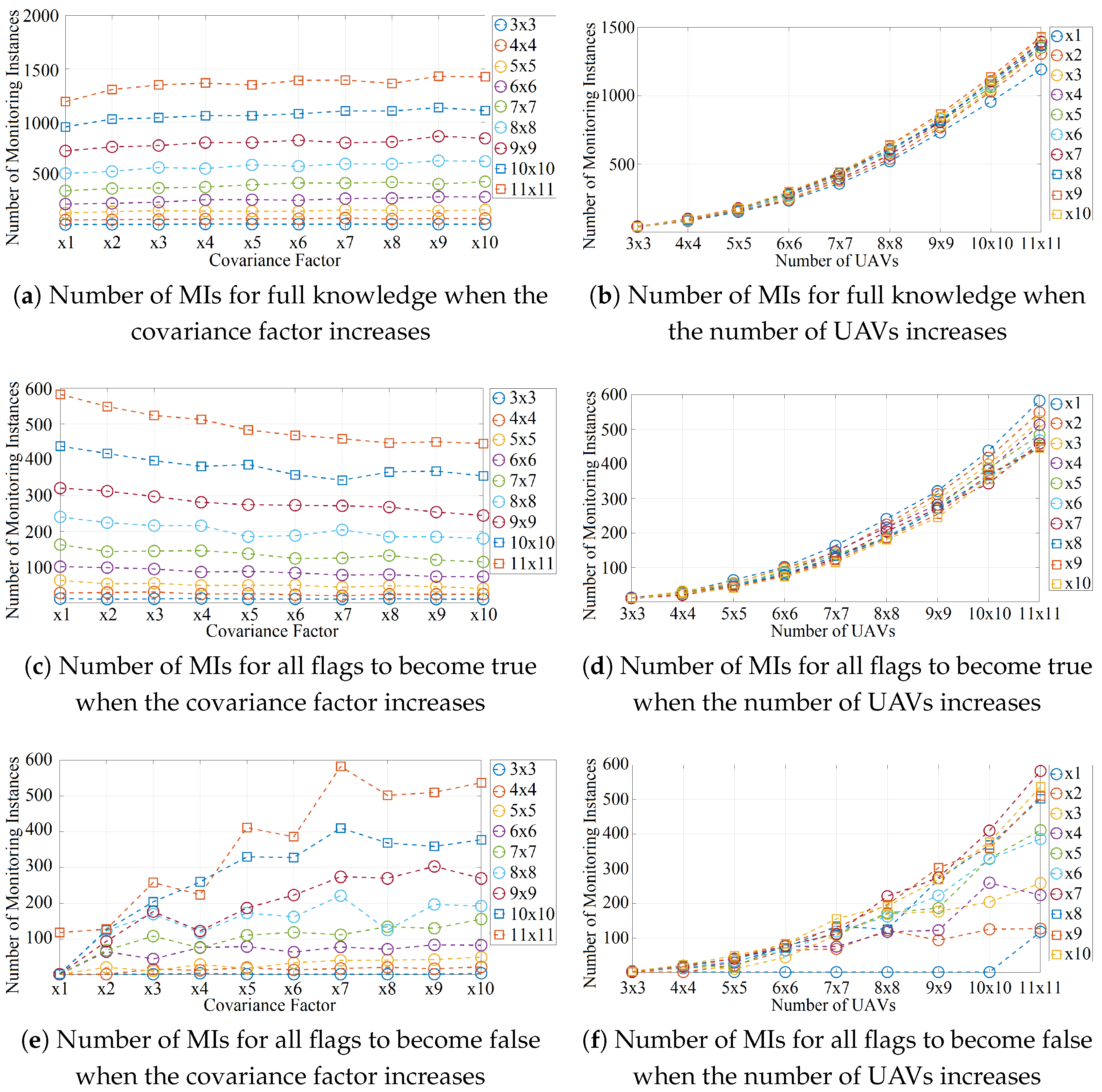
6.1.2. Grid Formation with an Increasing Covariance Factor
Figure 6 shows the number of MIs of the grid formation and when the clusters are more spread out. This is achieved by multiplying the diagonal of the covariance matrix by a scalar that we refer to as the
covariance factor. It takes integer values that increase from 1 to 10. Different sizes of grid formation are included, from
(
Figure 4) to
(
Figure 1a). In addition, in this case, only two target clusters are considered. Their centroids are shown in
Figure 4a. Their covariance matrices are
and
with 100 and 50 targets, respectively.
Figure 6a shows that the number of MIs for full knowledge increases slightly with the covariance factor, and the rate of increase is greater for larger grid sizes. When the grid size is
, the number of MIs increases from 1192 to 1425 as the covariance factor increases from 1 to 10. On the other hand, when the grid size is
, the number of MIs increases from 37 to 42.
Figure 6b shows the same data points as
Figure 6a but as a function of the grid size, not the covariance factor. The rate of increase is significant regardless of the covariance factor. The number of MIs increases from 37 to 1192 when the covariance factor is 1 and increases from 42 to 1425 when the covariance factor is 10.
Figure 6c shows that the number of MIs for all flags to become true decreases with the covariance factor and decreases faster when the size of the grid increases. At
, the number of MIs decreases from 583 to 445 as the covariance factor increases from 1 to 10. At
, the number of MIs decreases from 12 to 10. We attribute the decreasing trend to the larger area occupied by each cluster at larger factors. UAVs cover targets of multiple clusters at larger factors, facilitating the determination that the GMM parameters do not fit the target observations (i.e., all UAV flags becoming true). In other words, UAVs need to propagate knowledge further when clusters are covered by a small number of UAVs.
Figure 6d shows the same data points as
Figure 6c but as a function of the grid size, not the covariance factor. The rate of increase is again significant regardless of the covariance factor. The number of MIs increases from 12 to 583 when the factor is 1 and from 10 to 445 when the factor is 10.
The results of the grid formation in
Figure 6a–d are consistent with the results from the linear formation in
Figure 5. In both cases, the number of MIs is highly dependent on the diameter of the FANET. In other words, the number of MIs increases with the number of hops that need to be covered to relay knowledge from every UAV to other UAVs.
Figure 6e,f corresponds to the case that the GMM fits the ground observations, so the UAV flag values are expected to all be false.
Figure 6e shows that the number of MIs for all flags to become false increases with the covariance factor, and the rate of increase is greater for larger grid sizes. At
, the number of MIs increases from 0 to 3 when the covariance increases from 1 to 10. In fact, the number of MIs is 0 for all covariance factors less than 10, meaning that all UAVs start with the correct assumption that the GMM fits the observations (i.e., line 17 in Algorithm 1), and they do not override the initial assumption (lines 21 and 25). On the other hand, at
, the number of MIs increases from 118 to 536. Therefore, in this case, UAVs incorrectly override the initial assumption that the flag is false (line 17), changing its value to true (lines 21 and 25). However, after a number of MIs, all UAVs correctly determine that the flag is false.
Figure 6f shows the same data points as
Figure 6e but as a function of the grid size, not the covariance factor. The number of MIs increases in all cases of covariance factor values, and the rate of increase is greater for larger covariance factors. The number of MIs increases from 0 to 118 when the factor is 1 and increases from 3 to 536 when the factor is 10. This result is consistent with previous results. The number of MIs increases with the diameter of the FANET.
6.1.3. Grid Formation with an Increasing Number of Target Clusters
Figure 7 shows the number of MIs of the grid formation and when the number of clusters increases from two to nine, as shown in
Figure 4. Different sizes of grid formations are also included, from
(
Figure 4) to
(
Figure 1a).
Figure 7a,b shows the number of MIs for full knowledge. The differences between the subfigures in
Figure 6a,b are negligible. This is confirmation that the acquisition of full knowledge by all UAVs is dependent on the diameter of the FANET, not on the number of clusters or the covariance factor.
Figure 7c,d shows the number of MIs for all flags to become true. The results show the same trends as
Figure 6c,d with one difference. The number of MIs decreases faster with the number of clusters (
Figure 7c) than with the covariance factor (
Figure 6c). This means that the tests on lines 20 and 24 of Algorithm 1 are more sensitive to the number of clusters than the covariance factor. These tests compare
,
, and
with
, so the negative average log-likelihood given the UAV’s knowledge, agreement, or withheld knowledge is more sensitive to the number of clusters than the covariance factor.
It should also be noted that the faster decrease in the number of MIs in
Figure 7c than in
Figure 6c means that Algorithm 1 detects the unfitness of the GMM faster for larger numbers of clusters than for higher covariance factors. This observation is also valid for the number of MIs needed for all flags to become false.
Figure 7e,f shows the same trends as
Figure 6e,f with one difference. The number of MIs increases more slowly with the number of clusters (
Figure 7e) than with the covariance factor (
Figure 6e).
6.2. Performance Evaluation: Distributed EM Algorithm
The performance of the distributed EM algorithm is evaluated with the number of iterations of the while loop (i.e., line 5 of Algorithm 3) until the termination criterion is met. Given that one iteration consists of four for loops (i.e., lines 6, 9, 12, and 16), there are four rounds of communication on the wireless token-ring network per iteration.
In this case, we change our termination criterion to the same as the default criterion used in the centralized EM algorithm of the MATLAB Toolbox for Statistics and Machine Learning (i.e.,
fitgmdist in [
49]). This criterion allows us to use
fitgmdist to benchmark our distributed EM algorithm. The reason is that one EM step is completed per iteration of the
while loop of our distributed EM algorithm (i.e., line 5 of Algorithm 3). Therefore, both algorithms perform one EM step per iteration, making the comparison of the number of iterations fair.
The termination criterion is as follows. Let be the average negative log-likelihood at the iteration. The termination occurs when two conditions are met: (1) and (2) . This means that the new value of no longer decreases significantly, .
The distributed EM algorithm (i.e., Algorithm 3) and the MATLAB algorithm (i.e.,
fitgmdist [
49]) are also given the same initial GMM parameter values (i.e.,
in Algorithm 3) for a fair comparison. The values are calculated as follows. The weights
of
are uniform, i.e.,
. The centroids
of
are calculated using the MATLAB implementation of k-means. The covariance matrices
of
are set to diagonal matrices with two diagonal elements. The values of the upper and lower elements are the variance of the
x and
y coordinates of the targets of the
cluster determined from k-means.
Figure 8 shows the number of iterations of the linear formation when the number of UAVs increases from 2 to 15. Both cluster locations, centered and uncentered, and both algorithms, distributed (Algorithm 3) and centralized (fitgmdist [
49]), are evaluated in
Figure 8. Each data point in
Figure 8 is the average number of iterations of 20 simulations, with each simulation having a unique set of randomly generated targets. The number of iterations increases faster for the distributed EM algorithm than for the centralized EM algorithm as the number of UAVs increases. This result is expected because the centralized algorithm does not require DAC; all target observations are available to a single computing system, so the rounds of communication in Algorithm 3 are not needed in the centralized EM algorithm.
Figure 8 also shows that the location of clusters in the center of the image or in the boundaries of the image (i.e., centered vs. uncentered clusters shown in
Figure 3) does not have a significant effect on the number of iterations. The number of iterations increases at similar rates in both cases, centered and uncentered, and for both algorithms, centralized and distributed.
Figure 9 shows the number of iterations of the grid formation. Each data point is the average number of iterations of 20 simulations, with each simulation having a unique set of randomly generated targets.
Figure 9a shows the number of iterations when the number of clusters increases from two to nine at grid sizes that increase from
to
, including both distributed and centralized algorithms. The results are consistent with the linear configuration. The centralized EM algorithm converges with the lowest number of iterations in all cases. However, the trend of the centralized EM algorithm is to increase. On the other hand, the distributed EM algorithm tends to remain constant. There are exceptions, such as the
and
formations, which have decreasing and increasing trends, respectively, but the average trend when all grid sizes are considered is to remain constant.
Figure 9b shows the same data points as
Figure 9a but rearranged. In this case, the number of iterations is shown as the grid size increases from 3 × 3 to 11 × 11 at numbers of clusters that increase from 2 to 9. The general trend is for the number of iterations to increase with the grid size. This is expected because completing DAC requires more iterations when the data being averaged is distributed across a higher number of UAVs.
Figure 9b also shows exceptions to the general trend when the grid size increases from even to odd sizes (e.g., from 4 × 4 to 5 × 5). In other words, the number of iterations increases in both cases, even and odd, but grids of odd size converge faster. For example, the number of iterations is higher for a 10 × 10 grid than an 8 × 8 grid, and it is higher for an 11 × 11 grid than a 9 × 9 grid, but the 9 × 9 and 11 × 11 grids require fewer iterations than the 8 × 8 and 10 × 10 grids. We attribute this behavior to the effect that different network topologies have on DAC convergence [
50].
6.3. Comparison of the Monitoring and Distributed EM Algorithms with Related Work
To the best of our knowledge, distributed monitoring algorithms are based on a coordinator that collects data from nodes of the network as in [
3,
10,
11,
12,
13,
14,
15,
16,
17,
18,
19] covered in
Section 2, and our monitoring algorithm is based on [
20] to avoid the need for a coordinator. Therefore, the performance of our monitoring algorithm is not comparable to [
3,
10,
11,
12,
13,
14,
15,
16,
17,
18,
19]. The performance evaluation in [
20] did not cover the number of MIs needed for the nodes to propagate their local knowledge to determine the unfitness of the GMM. The framework closest to our monitoring algorithm is the gossip/consensus algorithm [
51,
52]. These algorithms also require a number of MIs to propagate local information across the network.
Table 2 compares the performance of Algorithm 1 [
51,
52].
Convergence in [
51] requires at least 1000 MIs in a network of 100 temperature sensor nodes of higher connectivity (i.e., lower diameter) than our
grid. Convergence in [
52] requires 12 MIs in a network of 7 UAVs in linear formation that determine the location of a target UAV detected by all monitoring UAVs under Gaussian noise. In our monitoring algorithm,
UAVs require no more than 600 MIs, according to
Figure 6c and
Figure 7c, and 7 UAVs in linear formation require 16 MIs, according to
Figure 5.
Our distributed EM algorithm is compared to the algorithms in [
22,
29] because, as explained in
Section 2, it is an adaptation of the algorithm in [
22] that uses MH weights as in [
29].
Table 3 compares the performance of Algorithm 3 [
22,
29].
The algorithm in [
22] was simulated for one scenario only: 100 nodes and 3 target clusters. The termination occurred when
, which is 10 times less tight than the termination criterion used in our simulations in
Section 6.2. The number of iterations until termination was 185. On the other hand, our distributed EM algorithm took 118 iterations for the same number of nodes and clusters (i.e.,
UAVs and 3 target clusters in
Figure 9). The algorithm in [
29] was also simulated for one scenario only: 50 nodes and 2 target clusters. The termination was at 100 iterations. Our algorithm ended with 30 iterations for
UAVs and 2 target clusters, according to
Figure 9.
7. Practical Considerations on a UAV Network
Our open-source network of autonomous UAVs is shown in
Figure 10a and documented in [
1]. Two adjacent thermal images captured with our UAVs are shown in
Figure 10b.
UAV-to-UAV communication takes place over the Zigbee network, which is used for low-power and low-bandwidth industry applications. Each UAV is a WiFi router that connects to its controller, a Raspberry Pi, and a laptop computer. The controller is to override the autonomous operation of the UAV in the case of unsafe flight maneuvers due to unexpected events such as bugs in our code development or loss of GPS. The Raspberry Pi is used to interface the thermal camera with the operating system of the UAV. The laptop computer is used to program the UAVs for autonomous operation.
The thermal images in
Figure 10b capture the same hotspot on the ground. The hotspot is partially covered on the left image and fully covered on the right image. In practice, adjacent images overlap due to geolocation errors and external factors such as wind. Hotspots are characterized by keypoints that are matched to each other to align the overlapping images. This operation is known as
point-set registration [
39]. All keypoints belong to the set of observations
defined in
Section 3, and their coordinates in meters with respect to a user-defined origin can be calculated from the UAVs’ telemetry (i.e., latitude, longitude, altitude, pitch, yaw, and roll) and the thermal camera’s fields of view and resolution.
Our preliminary work in [
53] measured the maximum packet rate on a Zigbee wireless link at 65 packets per second.
Algorithm 1 transmits
from
to each of its neighbors, one at a time (line 13 of Algorithm 1), and the maximum number of neighbors in our simulations is four. Therefore, Algorithm 1 spends
ms to complete all transmissions. The
and its neighbors are a total of 5 UAVs, and only one of them can transmit at a time not to interfere with each other. Therefore, five transmissions are
ms long. Consider the
grid flight formation. This is 49 UAVs. The number of MIs for all flags to become true is 140 on average, according to
Figure 6d. This means that Algorithm 1 takes
s at least to determine that all flag values are true when the flight formation is a
grid of 49 UAVs.
Algorithm 3 requires passing the token along the ring network four times per iteration. These four rounds of communication correspond to the
loops on lines 6, 9, 12, and 16 of the algorithm, and each UAV communicates with its neighbors in every round. Therefore, one iteration of Algorithm 3 in the
grid is
12,152 ms or 12 s long. Algorithm 3 converges after 30 iterations when there are 2 clusters of targets on the ground, according to
Table 3. This is 360 s or 6 min. The same calculation can be completed for a higher number of UAVs. For example, for the case of 100 UAVs (i.e.,
grid), Algorithm 3 converges after 120 iterations when there are 3 clusters of targets on the ground, according to
Figure 9a. Completing this number of iterations on a ring of 100 UAVs takes
s or 50 min, which is not practical. The Zigbee network would have to be replaced with a wireless network with higher data rates, such as WiFi, at the cost of higher power consumption.
The previous numerical analysis assumes ideal wireless links. It does not account for delays from lower layers of the protocol architecture: data-link and medium-access control layers. These delays can be significant when the number of neighbors increases (i.e., medium access control) and when packets are not received (i.e., data link). For example, one iteration of Algorithm 3 is 12 s long in the grid, so the convergence time increases by 12 s every time the token is lost due to a failed packet reception.
The analysis also neglects data processing time. Data processing is performed in Algorithm 1 to evaluate the average negative log-likelihood defined in (3) (lines 6, 7, 8, and 13). Data processing takes place on Algorithm 3 using the formulas in (3), (8), (12), (16)–(18). All formulas operate on observations in
, and thermal images such as those in
Figure 10b have a number of observations that do not exceed 350 in our data set. Each observation consists of two floating point numbers that correspond to the coordinates
x and
y. The evaluation of these formulas on this number of observations takes a fraction of a millisecond on our UAV platform. Therefore, data processing time is negligible with respect to UAV-to-UAV communication.
The power consumed for data processing and Zigbee radios [
53] is also negligible with respect to other aspects of UAV operation (e.g., propellers, flight controller, image processing, and WiFi).


