Article

Neural Adaptive Nonlinear MIMO Control for Bipedal Walking Robot Locomotion in Hazardous and Complex Task Applications

1
Laboratory of Aeronautical Sciences, Institute of Aeronautics and Space Studies (IASS), Blida 09000, Algeria
2
School of Digital and Physical Sciences, Faculty of Science and Engineering, University of Hull, Hull HU6 7RX, UK
3
Institute of Electrical and Electronic Engineering, Boumerdes 35000, Algeria
4
Department of Electrical and Computer Engineering, ZEP Campus, University of Western Macedonia, 50100 Kozani, Greece
*
Author to whom correspondence should be addressed.
Robotics 2025, 14(6), 84; https://doi.org/10.3390/robotics14060084
Submission received: 9 May 2025 / Revised: 7 June 2025 / Accepted: 12 June 2025 / Published: 17 June 2025
(This article belongs to the Section Humanoid and Human Robotics)

Abstract

:
This paper introduces a robust neural adaptive MIMO control strategy to improve the stability and adaptability of bipedal locomotion amid uncertainties and external disturbances. The control combines nonlinear dynamic inversion, finite-time convergence, and radial basis function (RBF) neural networks for fast, accurate trajectory tracking. The main novelty of the presented control strategy lies in unifying instantaneous feedback, real-time learning, and dynamic adaptation within a multivariable feedback framework, delivering superior robustness, precision, and real-time performance under extreme conditions. The control scheme is implemented on a 5-DOF underactuated R A B B I T robot using a d S P A C E D S 1103 platform with a sampling rate of t = 1.5   m s   ( 667   H z ) . The experimental results show excellent performance with the following: The robot achieved stable cyclic gaits while keeping the tracking error within e = ± 0.04   r a d under nominal conditions. Under severe uncertainties of trunk mass variations m t r u n k = + 100 % , limb inertia changes I l i m b = ± 30 % , and actuator torque saturation at τ = ± 150   N m , the robot maintains stable limit cycles with smooth control. The performance of the proposed controller is compared with classical nonlinear decoupling, non-adaptive finite-time, neural-fuzzy learning, and deep learning controls. The results demonstrate that the proposed method outperforms the four benchmark strategies, achieving the lowest errors and fastest convergence with the following: I A E = 1.36 , I T A E = 2.43 , I S E = 0.68 , t s s = 1.24   s , and M p = 2.21 % . These results demonstrate evidence of high stability, rapid convergence, and robustness to disturbances and foot-slip.

1. Introduction

Bipedal locomotion has long been central to robotics and biomechanics, aiming to replicate human-like walking. A major challenge has been ensuring dynamic stability, addressed early on by Gubina [1], who introduced analytical models based on the inverted pendulum. This framework became foundational for later stability assessments and advanced control techniques [2]. Lyapunov’s second method [3] added mathematical rigor to postural equilibrium, while feedback-based on–off control [4] marked early practical implementations. Modeling-constrained dynamic systems further integrated stability into robotic biped design [5]. Throughout the late 20th century, strategies evolved via pole assignment, on–off feedback, and constrained modeling [6,7,8,9]. Saleem [10] and Afifa [11] introduced fractional-order and sliding-mode control for better adaptability. Later, optimization and intelligent control—e.g., genetic algorithms [12], terrain adaptation [13], other adaptive systems [14,15]—boosted robustness. Dariush [16] enhanced gait precision via external measurement-based motion analysis.
Recent work by Chevallereau [17,18,19] on underactuated bipedal locomotion, Grizzle’s nonlinear control frameworks [20], and Djoudi’s optimal motion planning [21,22,23] emphasized the role of zero moment point (ZMP) in dynamic stability [24,25]. Neural networks and machine learning [26,27] have improved adaptability to environmental changes. Feedback control advances by Westervelt [28], Djoudi [29], and Chevallereau [30,31] further enhanced dynamic stability. Grizzle [32] addressed challenges in 3D locomotion, spurring new control methods. For human-like gait, Wang [33] and Liu [34] introduced foot rotation and toe support, improving energy efficiency, Hemami [35] introduced human and robotic movement in the air. Kim [36] and Kakaei [37] developed robust, whole-body control strategies, aiding real-world humanoid applications. Passive dynamics were explored by Martínez and Villarreal-Cervantes [38], while fuzzy logic [39] and deep learning [40] expanded adaptability in varied conditions.
Modern advancements continue to push the boundaries of bipedal locomotion, incorporating bio-inspired control strategies to enhance gait stability and adaptability. Wu [41] proposed a bionic walking control approach based on central pattern generators (CPGs), utilizing an improved particle swarm algorithm to refine locomotion patterns. Extending this research, Wu [42] introduced a multivariate linear mapping technique for stabilizing CPG-based control, further improving adaptability in dynamic environments. Additionally, passive tendon mechanisms [43] and hybrid control methodologies that blend adaptive techniques with conventional feedback control have been explored to optimize gait efficiency and stability [44]. Mou [45] introduced high-dynamic bipedal robots featuring underactuated telescopic straight legs, enhancing both agility and adaptability. Furthermore, model-predictive control strategies [46,47] have been investigated to achieve more natural and efficient gait dynamics. These ongoing developments underscore the continuous effort to bridge the gap between theoretical control frameworks and practical walking robot applications.
A key gap in the current literature is the absence of a real-time, adaptive control framework that seamlessly combines trajectory planning, dynamic modeling, instantaneous feedback, and hybrid gait transitions for bipedal robots operating in uncertain and dynamically changing environments. Motivated by the persistent limitations of existing neural adaptive MIMO control strategies, particularly their inability to maintain stability under structural damage, abrupt disturbances, or partial system failures, this work proposes a unified and robust control solution. Unlike fragmented approaches that separately address adaptation, learning, and feedback correction, our framework tightly integrates these components in real time to enhance performance in dynamically changing environments. In summary, the primary novel contributions of the proposed control method of this work are as follows:
  • Unified adaptive control: Combines adaptation, learning, and real-time feedback within a cohesive architecture, addressing the fragmentation in prior methods.
  • Robustness under critical failures: Maintains gait stability under severe conditions, including structural damage, disturbances, and system degradation.
  • Real-time feedback and learning: Achieves fast correction using finite-time dynamic feedback and RBF-based online learning in hazardous tasks.
  • Synergistic adaptation and learning integration: Combines MIMO adaptive control and neural approximation for precise trajectory tracking under uncertainty.
  • Scalability and generalization: Applicable across diverse walking modes and robotic platforms, extending its use beyond the tested 5 DOF RABBIT robot.
This paper is organized as follows: Section 2 describes a bipedal robot and its dynamic models for various walking phases, including single support, impact dynamics, symbolic modeling, and trajectory generation. Section 3 presents the control strategy, combining nonlinear decoupling with finite-time convergent control, and it includes hybrid dynamics analysis via the Poincaré method and a neural network-based adaptive framework. Section 4 reports the experimental results of the RABBIT robot across three scenarios. Section 5 concludes with key insights and future directions.

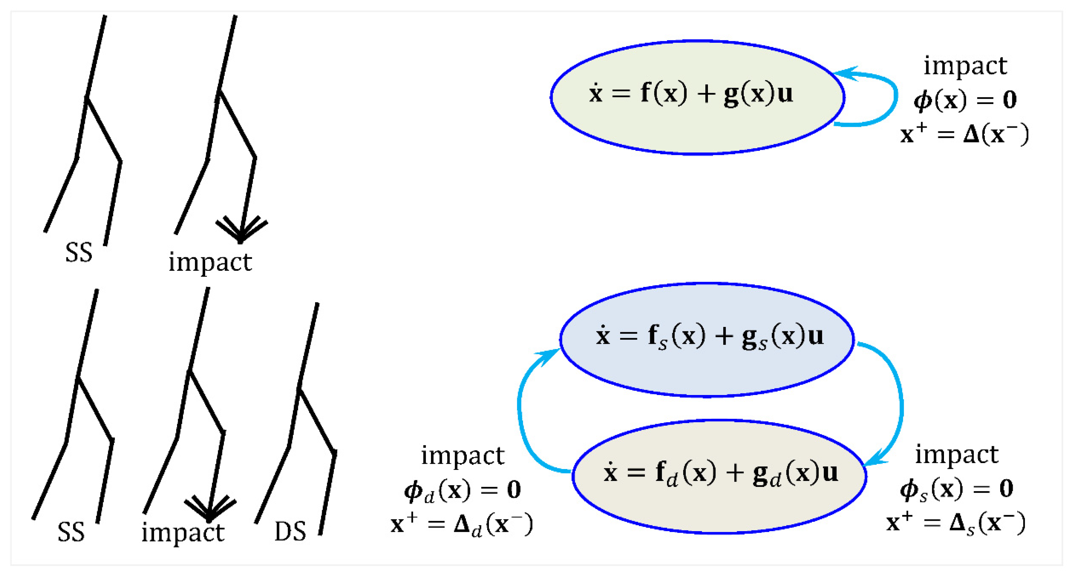
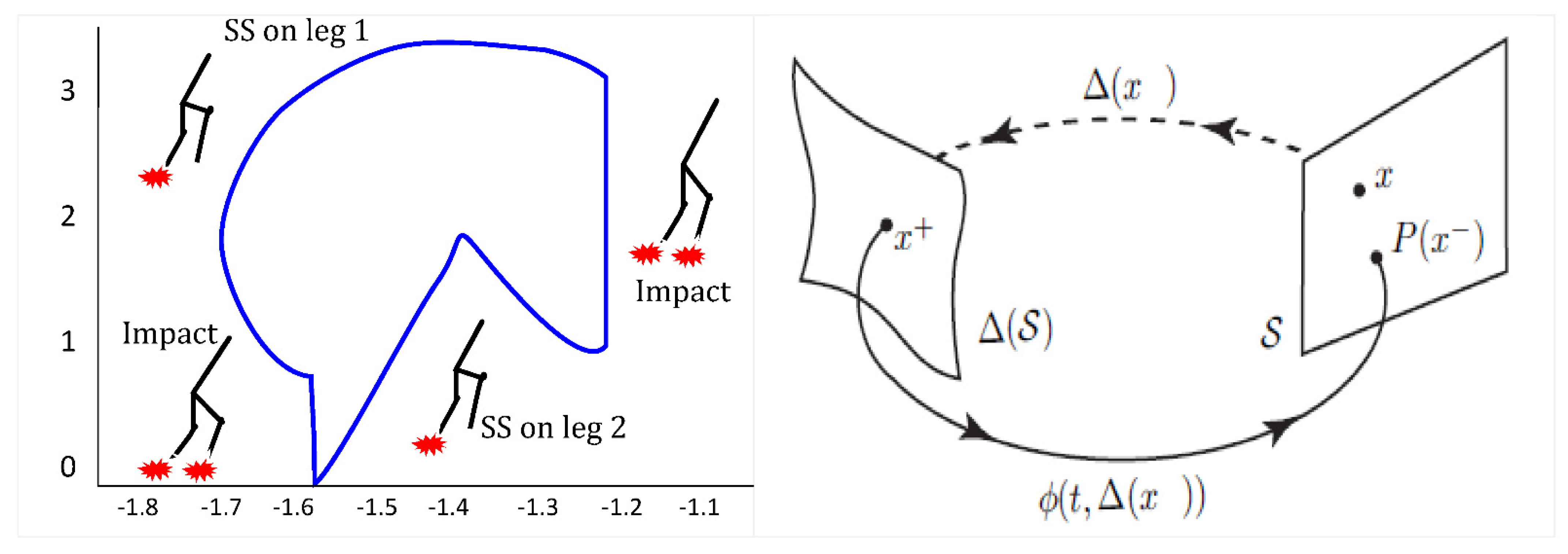
2. Mathematical Modeling of Bipedal Locomotion

This section deals with the control of bipedal walking robots, with an application to the planar RABBIT prototype robot with un-motorized ankles. Efforts have focused on the control and generation of reference trajectories, defined in the joint geometric space, allowing stable cyclic walking (see Figure 1) in a context of underactuation [31].
Walking is the alternating repetition of elementary movements from one leg to the other, resulting in a cyclic pattern that can be described in two ways. It is best modeled as a sequence of steps—elementary reference motions executed in various forms but defined by fixed kinematic properties. Each step consists of two distinct phases:
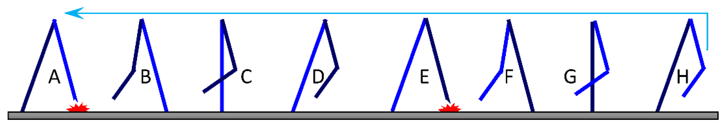
Single-support phase or swing phase, during which the locomotion system evolves as an open kinematic chain (one foot on the ground and the other is free).
Double-support phase, during which the locomotion system moves as a closed kinematic loop (both feet on the ground).
The single-support phase, a transfer phase, spans from the toe-off to heel-touch of the swing leg. Double support extends from the heel-touch of the front foot to the toe-off of the rear foot. In this phase, the system becomes overactuated, and its dynamics is underdetermined, requiring specialized methods to manage actuation redundancies [28].

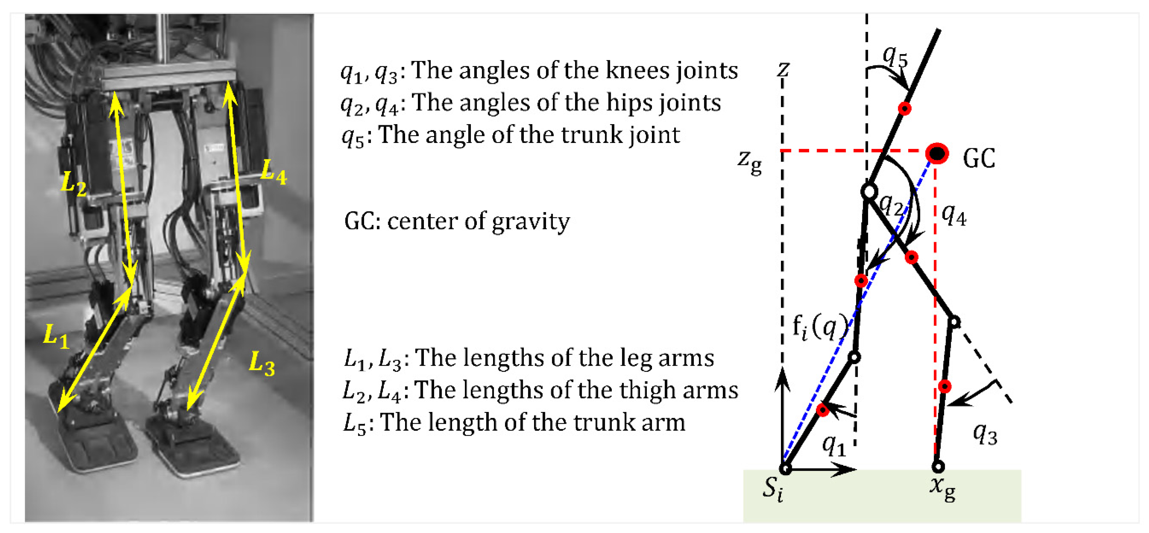
2.1. Kinematic and Dynamic Modeling of Biped Robots (Diff Phases)

The Lagrange equations give the dynamics of the system directly in the joint space q R n in the following vector form:
d d t L q ˙ L q = Q e x t
where
Q e x t t is the vector of generalized forces/torques;
L = E k E p is the L a g r a n g i a n of the system;
E k t   a n d   E p t are the total kinetic and potential energies of the system;
q t   a n d   q ˙ t are the vectors of the generalized positions and velocities.
From the Lagrangian, the equations of motion are as follows [25]:
d d t E k q ˙ E k q + E p q = Q e x t = D q , q ˙ + B T Γ + J λ
where λ is the Lagrange multiplier vector, and J is the Jacobian matrix of constraints. The last equation gives the following (see [48,49]):
A q q ¨ + C q , q ˙ q ˙ + G q = Q e x t   e q u a t i o n   o f   m o t i o n
where A (n × n) is the inertia matrix. C (n × n) corresponds to Coriolis and centrifugal effects. G (n × 1) corresponds to the effects of gravity. Matrices A , C , and G are given by:
A q = 2 E k q ˙ 2 ;   G q = E p q ;   C q , q ˙ = C i j ; C i j = k = 1 n c i , j k q ˙ k   c i , j k = 1 2 A i j q k + A i k q j A j k q i
The defining characteristic of a walking robot is the repetitive and alternating contact of its legs with the ground, making it a fundamental aspect of locomotion (Figure 2). Accurately modeling this contact is essential to account for the constraints imposed by the robot’s interaction with its environment. These constraints dictate the behavior of the foot during ground contact, ensuring that it neither lifts off nor slips, thereby maintaining stable and controlled movement.
In rigid contact (un-deformable ground), foot velocity and acceleration are zero and enforced by unknown contact forces. In compliant contact, forces depend on the ground’s deformation and its rate. The position χ i = x χ i ,   y χ i R 2 × 1 of the tip S i of the supporting foot (Figure 3) is a function of the joints q = q 1   q 2   q 3   q 4   q 5 R 5 × 1 and the position of the center of gravity (CG) according to the following: x g z g = χ i + f i q . The vector f i q = f i x ,   f i y R 2 × 1 is only a function of q and the parameters of the robot (lengths of the bodies and positions of the centers of gravity). In rigid contact, foot i , which is resting on the ground, is fixed. Its position χ i is constant, and depending on the type of contact, its orientation can also be constant. This results in an equation of the following type: χ i q = c ; here, q is the vector of generalized coordinates describing the biped, and i = 1,2 is the index. The number and type of equations written in equation ( χ i q = c ) depend on the type connection that exists between the foot in contact and the ground. The zero velocity/acceleration constraints are written by differentiating χ i = c :
χ i = c χ ˙ i q = A c i q x ˙ = 0   χ ¨ i q = A c i q x ¨ + H i q , q ˙ = 0     w i t h   A c i = χ i x = f i q   I 2 R 2 × 7
where x = q T   x g   z g R 7 × 1 , and A c i q = χ i q / x is the Jacobian matrix of χ i with respect to x . H i q , q ˙ contains the other terms appearing during the derivation. With fixed foot contact, foot velocity and acceleration are at zero.
The considered robot is an “underactuated RABBIT” prototype model presented in Figure 3. The biped is composed of five bodies (links), a trunk, and two identical legs. Each leg consists of two bodies articulated at the knee. Knees and hips are pivot joints assumed to be frictionless and without mechanical play. The vector of generalized coordinates x = q 1   q 2   q 3   q 4   q 5   x g   z g , which describes the configuration of the biped, is composed of q c = q 1   q 2   q 3   q 4 R 4 × 1 of the relative-angle motors defining the shape of the robot and q a = q 5   x g   z g R 3 × 1 , defining the situation of the trunk of the robot with respect to a fixed frame in the vertical plane ( x , z ) . q 5 is the absolute orientation of the trunk, and x g and z g are the coordinates of the center of mass of the biped. The robot’s position is described by its center of gravity, simplifying impact modeling and integrating it into the system’s dynamics. The biped, powered by four motors, has joint torques Γ = Γ 1   Γ 2   Γ 3   Γ 4 acting on the knees and hips (see Figure 4 and Figure 5 [25,28,31]).
Table 1 lists the RABBIT robot’s dynamic and geometric parameters [19,21]:
  • m i is the mass of the i t h body i = 1 7 (if we neglect feet, then i = 1 5 ).
  • I G i is the i t h moment of inertia at the center of gravity along axis y .
  • I A i is the moment of inertia of motor i around the y axis.
  • s i is the distance from body i ’s center of gravity to its frame origin.
The 7 DOF dynamic model of the robot is given according to the Lagrange formalism by the general equation of motion. With our choice of coordinates, we have [22,29]
E k = 1 2 x ˙ t A 5 q c 0 5 × 2 0 2 × 5 m I 2 × 2 x ˙ t ; E p = m g z g   Q e x t t = D q , q ˙ + q c x Γ t + i = 1 2 δ χ i δ x R i  
where m is the total mass of the biped, g is the gravity acceleration, and A 5 q c R 5 × 5 is the inertia matrix. D q , q ˙ R 7 × 1 is a vector that regroups the terms of dissipative forces at the joints. R i denotes ground reaction forces. Notice that A q c x ¨ + C q , q ˙ x ˙ + G q = Q e x t , so we can write
D q , q ˙ + B Γ + J λ = D q , q ˙ + q c x Γ + A c 1 q R 1 + A c 2 q R 2
where A q c R 7 × 7 is the symmetric positive–definite inertia matrix, which defines kinetic energy. C q , q ˙ R 7 × 7 is a matrix that groups the centrifugal and Coriolis inertia terms together. G q R 7 × 1 represents the terms of gravity. D q , q ˙ R 7 × 1 is a vector that regroups the terms of dissipative forces at the joints, and B R 4 × 7 . The presented model is convenient for all phases of planar bipedal locomotion. For double-support phases, both ground reactions are not zero. For single-support phases, only one reaction force is not zero. For flight phases, both reaction forces are zero. The direct dynamic model of the RABBIT robot during the single-support phase has four joint couples Γ = Γ 1   Γ 2   Γ 3   Γ 4 as inputs and the state vector of the robot q = q 1   q 2   q 3   q 4   q 5   . With respect to q ˙ = q ˙ 1   q ˙ 2   q ˙ 3   q ˙ 4   q ˙ 5 , this model is the robot simulator, at its output gives the real articular acceleration x ¨ t with x = q   x g   z g and the ground reaction force R i . In this section, we provide the calculation of this model. The equations of motion governing the robot when it is in the single-support mode can be deduced from Equation (6). If we consider that the biped is resting on foot 1, there is only one force from the reaction of two components, R 1 = R 1 x ,   R 1 z , and the friction torque is zero at R 2 = 0 ,   0 . The dynamic model is written as follows:
A q c x ¨ + C q , q ˙ x ˙ + G q = B Γ + A c 1 q R 1 ;     A q c = b l k d i a g A 5 q c   m I 2 × 2
The model comprises seven differential equations, and we have nine unknowns, which are joint acceleration x ¨ with seven components and the two components of the force of reaction R 1 = R 1 x ,   R 1 z . This system can be completely defined by writing the stress equation with respect to the foot in contact with the ground. The foot in contact must not slip or take off, so its position is constant, and therefore, its speed and acceleration are zero. Thus, we have the position of the foot in support denoted by χ 1 t , and it is as follows: χ 1 t = c o n s t ; χ ˙ 1 = 0 ; χ ¨ 1 = 0 . We deduce, analogously to the kinematic and dynamic constraints, A c 1 q x ˙ t = 0 and A c 1 q x ¨ + H 1 q , q ˙ = 0 , where H 1 q , q ˙ = A c 1 q x ¨ is a matrix of dimension 2 × 1 , and A c 1 q is given as A c 1 q = f 1 q / q I 2 . By combining the equations of the dynamic model and the second equation’s constraint on the acceleration of the foot in support, we obtain a ninth-order system, A q c x ¨ A c 1 q R 1 = B Γ C q , q ˙ x ˙ G q , with A c 1 q x ¨ + H 1 q , q ˙ = 0 . Thus, acceleration x ¨ and the reaction force R 1 are given by the following [17,18,19,30]:
x ¨ R 1 = A q c A c 1 q     A c 1 q 0 2 × 2 1 B Γ C q , q ˙ x ˙ G q H 1 q , q ˙ ; A q c = A 5 q c 0 5 × 2 0 2 × 5 m I 2 × 2 ;   B = I 4 × 4 0 3 × 4
In the case of single-phase support, we will use the 5 DOF model:
A 5 × 5 q q ¨ + C 5 × 5 q , q ˙ q ˙ + G 5 × 1 q = Γ 0

2.2. The Model of Impacts

Impacts are modeled as high-intensity forces acting over an infinitesimal time t , represented by the integral of the contact force during this interval. Since t is very small, positional changes are neglected. Thus, impact causes a sudden change in velocity and not position, and it is often expressed using a Dirac function scaled by the impulse’s magnitude. The goal is to compute post-impact velocities and impulses, assuming that pre-impact velocities are known. At the end of single support, when swing leg j contacts the ground, an inelastic impact occurs. The ground reaction is modeled as a Dirac delta-function with intensity I R j , and the foot’s velocity is assumed to drop to zero immediately after contact. Depending on whether the stance leg lifts off, two types of impact may occur. The rebound between two links is classically described by the coefficient of restitution ε , which—via Newton’s impact law—relates the normal component of their relative velocity before and after impacts. For foot–ground collision during walking, it becomes v i n + = ε v i n , where v i n is the normal velocity upon contact. The value of ε , ranging from 0 (perfectly inelastic) to 1 (perfectly elastic), depends on the contact materials. By integrating the dynamic equations over an infinitesimal impact duration, the impulsive dynamics governing this phase can be derived. Since the matrices A q c and A c j q depend solely on the robot’s configuration, they are considered constant over the short collision duration. The resulting impact model is expressed as follows: A q f x ˙ + x ˙ = A c j q f I R j .
A 5 q f 0 5 × 2 0 2 × 5 m I 2 × 2 x ˙ + x ˙ = f j q / q I 2 × 2 I R j
Here, the superscripts (+) and (−) denote post- and pre-impact velocities, respectively, while q f represents the final configuration of the single-support phase. The contact forces, being theoretically infinite upon impact, yield finite impulsive effort I R j when integrated over the vanishing impact duration. The acceleration of the robot is taken as infinite, and by integrating it, we obtain the velocity variation x ˙ + x ˙ . As A q f is invertible, the velocity after impact is x ˙ + = x ˙ + A q f 1 A c j q f I R j , so we obtain A c j q f x ˙ + = A c j q f x ˙ + A c j q f A q f 1 A c j q f I R j . When matrix A c j q f is of full rank, this equation enables us to calculate I R j under the assumption that ( A c j q f x ˙ + = 0 ), so I R j = A c j q f A q f 1 A c j q f 1 A c j q f x ˙ . Moreover, one can derive an alternative formulation without the use of x ˙ (see [23,25]). First, we define δ q = q ˙ + q ˙ ; then,
A 5 q f δ q = m f j q f q x ˙ g + x ˙ g z ˙ g + z ˙ g = m f j q f q f j q f q q ˙ + f i q f q q ˙
Thus, the biped angular velocity vectors before and after impact are related by linear equation q ˙ + = q f q ˙ , where q f = 1 1 q f 2 q f   w i t h
1 q f = A 5 q f + m f j q f q f j q f q ; 2 q f = A 5 q f + m f j q f q f i q f q
The impulse efforts are modeled by Formalsky’s equation (see [17,25]):
I R j = m f j q f q q f f i q f q q ˙
A walking gait consists of alternating single-support, impact, and double-support phases. The system state η t , comprising configuration and velocity variables, evolves according to a hybrid model η ˙ t = f η t + g η u   w h e n   η t S , and η t + = ϕ η t   w h e n   η t S . Here, u is the control input, and f , g , and ϕ are nonlinear continuous functions. The impact set S defines the switching surface containing all states that trigger a ground impact. The second expression (as given by Westervelt and Chevallereau) models the instantaneous velocity change at impact (see [28]).
During single support, the robot evolves under a continuous dynamic model. An impact is detected when the swing foot reaches ground level ( ϕ = 0 ), causing a discontinuous change in velocity. This is followed by either single or double support on the opposite foot (see Figure 6). The double-support phase ends through a control-triggered vertical acceleration that lifts the foot off the ground.

2.3. Symbolic Calculations of the Model

During the initial and final single-support configurations and the double-support phase, both feet of the robot are in contact with the ground. These two feet thus form a closed kinematic loop. Three parameters are sufficient to determine these configurations: the distance between the feet d , the abscissa of the hip x h , and the height of the hip z h .
Now, we present the geometric model to express joint variables in terms of Cartesian variables. To simplify calculations, we define the absolute angle α i on the robot (see Figure 7) and compute them based on Cartesian parameters z h , x h , and d . A change in variable allows expressing the geometric model in terms of relative variables used for dynamics.
We decompose our calculation on the two legs, and the benchmark with respect to which all calculations are performed is related to the ankle of the rear support leg. The loop closure makes it such that the height of the hip, z h , is the same for the two legs, and the distance d between the legs is constant. This leads to the following constraints: x h = L 1 S α 1 + L 2 S α 2 ; z h = L 1 C α 1 + L 2 C α 2 ; d x h = L 3 S α 3 + L 4 S α 4 ;   a n d   z h = L 3 C α 3 + L 4 C α 4 , where S = sin and S = cos . In Table 1, we have lengths L 1 = L 2 = L 3 = L 4 ; this equality can greatly simplify calculations, but we prefer to keep different lengths to generalize the calculation and leave the choice of adding robustness to others. From the inverse geometric model, we have absolute angles α 1 , α 2 , α 3 , and α 4 in the function of step length d , the abscissa of the hip x h , and the height of the hip z h . We already have the absolute angle q 5 , which is also known. We obtain the following relations: q 5 + q 2 + α 2 = π , q 5 + q 4 + α 4 = π , q 5 + q 2 + q 1 α 1 = π and q 5 + q 2 + q 1 + α 3 = π     q 1 = α 1 + α 2 , q 2 = π q 5 α 2 , q 3 = α 4 α 3 , and q 4 = π q 5 α 4 . With angle q 5 being known, we have a system of four equations, and four unknowns can be solved easily to give us the expressions of the required positions:
p f 1 = 0 0 ; p g 1 = p f 1 + L 1 sin q 5 + q 2 + q 1 cos q 5 + q 2 + q 1 ; p h = p g 1 + L 2 sin q 5 + q 2 cos q 5 + q 2 p g 2 = p h + L 4 sin q 5 + q 4 cos q 5 + q 4 ; p f 2 = p g 2 + L 3 sin q 5 + q 3 + q 4 cos q 5 + q 3 + q 4
where p f 1 is the position vector of the first foot (first leg), p f 2 is the position vector of the second foot (second leg), p g 1 is the position vector of the first knee, p g 2 is the position vector of the second knee, and p h is the position vector of the hip.
The center of mass of each arm can be calculated from the previous relation by
p c 1 = p f 1 + s 1 L 1 sin q 5 + q 2 + q 1 cos q 5 + q 2 + q 1 ; p c 2 = p g 1 + s 2 L 2 sin q 5 + q 2 cos q 5 + q 2 p c T = p h + s 5 sin q 5 cos q 5 ;     p c 4 = p h + s 4 sin q 5 + q 4 cos q 5 + q 4 ;   p c 3 = p g 2 + s 3 sin q 5 + q 4 + q 3 cos q 5 + q 4 + q 3
The total C G of the robot is: p g = m 1 p c 1 + m 2 p c 2 + m 3 p c T + m 4 p c 4 + m 5 p c 3 / m , with m = m 1 + + m 5 . The coordinates of the feet and C G in the absolute frame are
P g = q 6 , q 7 T ; P f 1 = P g p g ; P f 2 = P f 1 + p f 2 ;         P c 1 = P f 1 + p c 1 ; P c 2 = P f 1 + p c 2 ; P c T = P f 1 + p c T ;         P c 3 = P f 1 + p c 3 ; P c 4 = P f 1 + p c 4 .  
The potential energy is: Ep = g[0 1] m 1 P c 1 + m 2 P c 2 + m 5 P c T + m 4 P c 4 + m 3 P c 3 . The absolute joint velocities are as follows: ω a 1 = q ˙ 5 + q ˙ 2 + q ˙ 1 ; ω a 2 = q ˙ 5 + q ˙ 2 ; ω a 3 = q ˙ 5 + q ˙ 4 + q ˙ 3 ; ω a 4 = q ˙ 5 + q ˙ 4 and ω a T = q ˙ 5 . The linear velocity of the center mass of each body is given by
v c 1 = P c 1 q q ˙ ; v c 2 = P c 2 q q ˙ ; v c 3 = P c 3 q q ˙ ; v c 4 = P c 4 q q ˙ ; a n d v c T = P c T q q ˙
The kinetic energies of each body of the RABBIT robot are
E k j = 1 2 m j v c j T v c j + I j ω a j 2 + I A j q ˙ j 2 ; f o r   j = 1 4   a n d   E k T = 1 2 m 5 v c T T v c T + I 5 ω a T 2
Thus, we have E k = E k 1 + E k 2 + E k T + E k 3 + E k 4 , with I j = I j 0 m j s j 2 and I 5 = I 50 . The matrices of the 7 DOF RABBIT robot model during single support were computed using MATLAB’s (R2023) symbolic toolbox (see Appendix A). Figure 8 clearly shows the detailed modeling flowchart, from defining symbolic variables to deriving the system matrices via the L a g r a n g i a n .

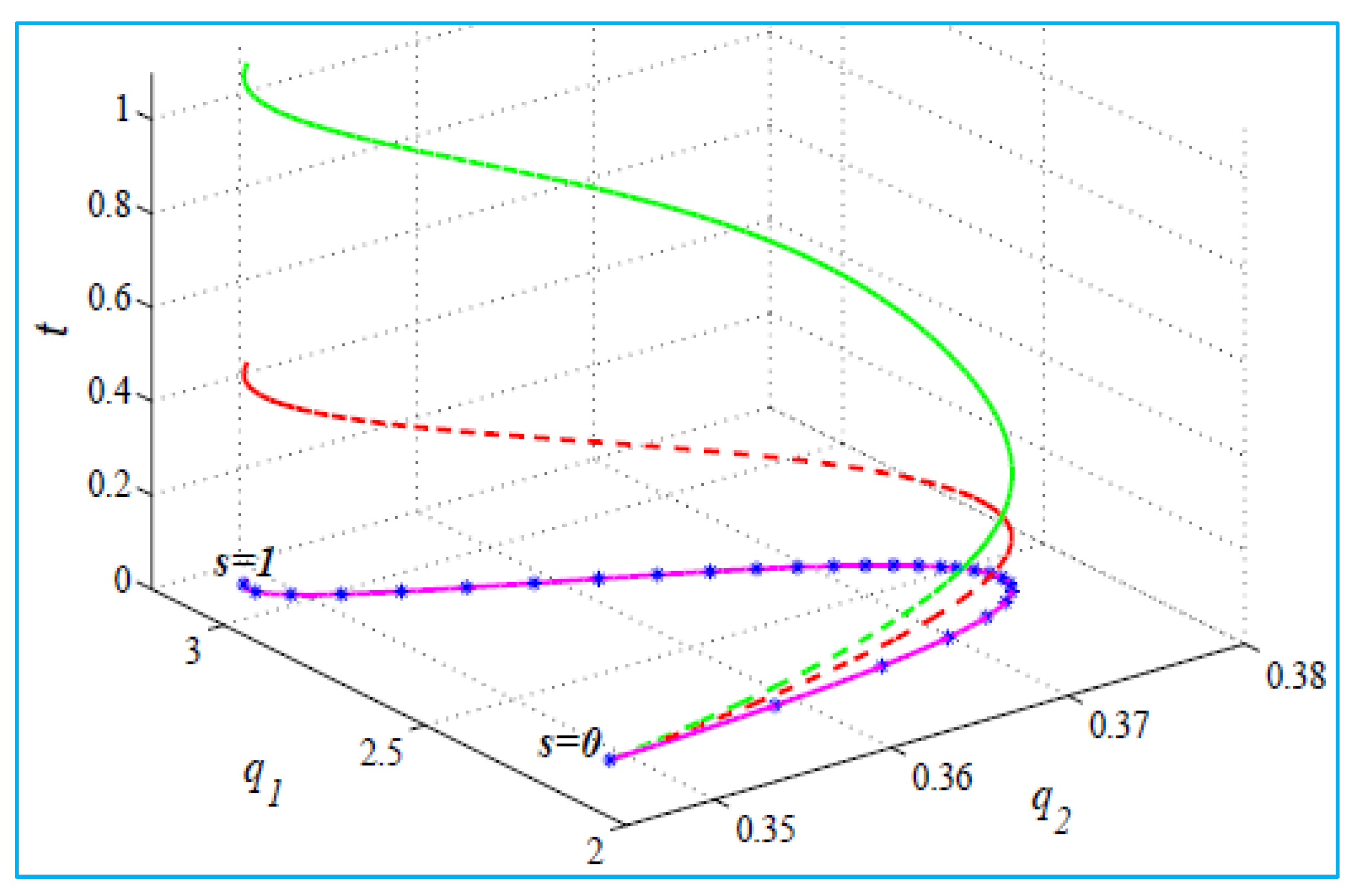
2.4. Optimal Trajectories Generation

Generally, in robotics, the reference trajectory is a motion written as a function of time for different link positions and velocities. This is valid for all types of fully actuated robots, but in our case, the five degrees of freedom is not fully motorized during the single-support phase. The four angles q 1 q 4 are motorized, but the rotation about the standing leg is free. For such cases, many solutions have been proposed in the literatures. The robot will track polynomial reference trajectories written in terms of curvilinear abscissa s 0   1 , which is
q d   t = q d   s t , q ˙ d   t = d q d   s   d s s ˙ a n d q ¨ d   t = d 2 q d   s   d s 2 s ˙ 2 + d q d   s   d s s ¨
  • Here, q d   0 = initial configuration, and q d 1 = final configuration.
  • For the first single support, the two legs change their roles from one step to another q d   0 = E q d 1 , where the matrix E = e 3   e 4   e 1   e 2   e 5 R 5 × 5 is the permutation matrix. The trajectory in polynomial form is q d s = α 0 + α 1 s + α 2 s 2 + α 3 s 3 + α 4 s 4 , and q ˙ d   s = α 1 + 2 α 2 + 3 α 3 s 2 + 4 α 4 s 3 s ˙ t . The optimal values of q d   s , q ˙ d   s are given in [21]. Figure 9 shows how joint motion differs from the path.
The coefficients can be obtained by (according to [25])
α 0 α 1 α 2 α 3 α 4 = 16 16 I 5 16 I 5 16 I 5 0 5 0 5   0 5 4 I 5 16 I 5 16 I 5 16 I 5   0 5 4 I 5 I 5 0 5 32 I 5   0 5 2 I 5 16 I 5 0 5 48 I 5   0 5 I 5 16 I 5 0 5 64 I 5 1 q d s = 0   q d s = 0.5   q d s = 1   d q d / d s s = 0 d q d / d s s = 1

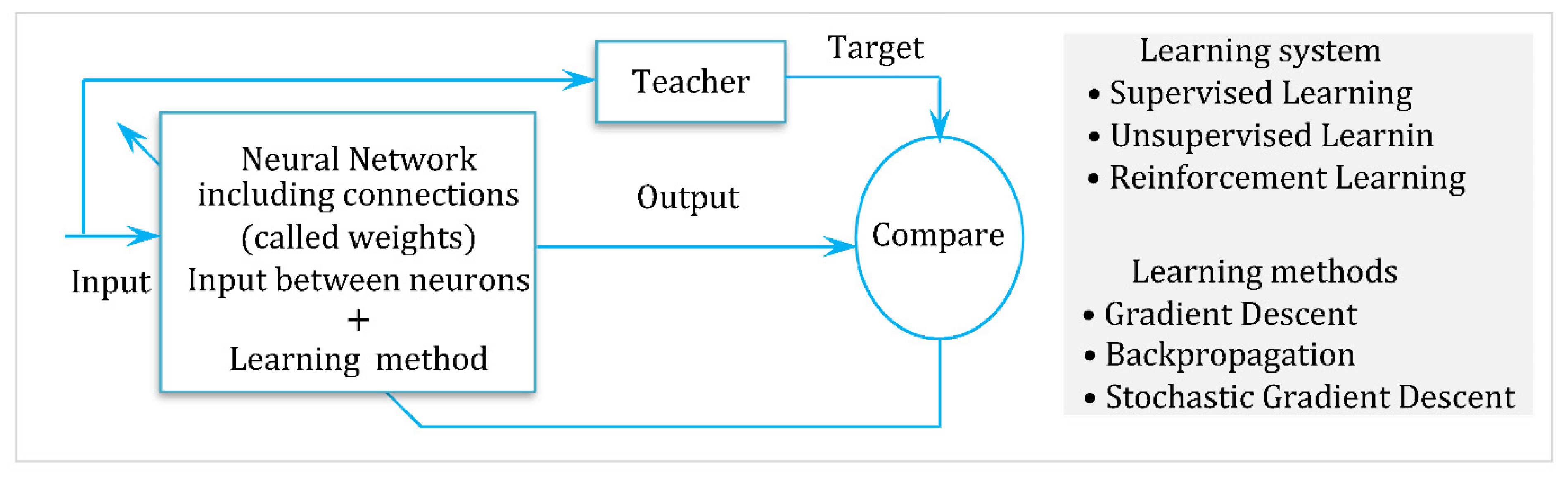
3. Basics of Intelligent Adaptive Control and Neural Networks

The dynamic modeling of walking robots via Lagrange–Euler methods and its finite time convergent control is complex and error-prone due to underactuation, multi-link setups, and hybrid phases [50,51]. Neural networks (NNs) provide a data-driven alternative, with feedforward architectures approximating nonlinear dynamics. However, static networks cannot handle time-varying control, requiring dynamic NNs that capture system evolution. These are computationally intensive and prone to overfitting. Structure-aware algorithms help reduce the degrees of freedom. Parameter-linear models like RBF networks, despite their universal approximation capabilities, face the curse of dimensionality. Exploiting known system structures allows static, compact networks to efficiently approximate robot dynamics, offering better generalization, lower computational costs, and suitability for real-time control [52,53,54,55].

3.1. Neural Networks and Global Approximation Theory

Neural networks are composed of interconnected nodes (or neurons) linked by weighted connections, where the weights serve as trainable parameters. The specific arrangement of nodes and interconnections defines the network architecture, which varies across models and must be selected carefully based on the target application. As network capabilities differ by structure, choosing an appropriate architecture is essential for achieving optimal performance in a given control or modeling task.
Definition 1.
(Function Approximation): If   f x : R n R m is a continuous function in a compact set   Ω x and   y W , x : R s × R n R m is an approximating function that depends continuously on   W and x , then the approximation problem is to determine the optimal parameter W for some metric (or distance function) d such that d y W , x , f x ϵ for an acceptable small e [53].
In function approximation, a neural network defines an estimator y W , x for an unknown function f x , where the weight W is adjusted to minimize output errors over a training dataset. This involves two core challenges: the representation problem, which concerns selecting a suitable function structure y W , x , and the learning problem, which focuses on optimizing W to best match the target function. A neural network is a parallel, distributed computational model composed of simple processing units capable of learning from experience and storing knowledge through training. It mimics the brain in two key ways: learning occurs through interaction with the environment, and acquired knowledge is encoded in the synaptic weights connecting the neurons. A neuron serves as the fundamental processing unit of a neural network. Its structure is illustrated in Figure 10, and it provides the foundation for constructing a wide range of neural network architectures.
Claim 1.
If A C K , R n is an algebra of continuous vector-valued function f that separates points and contains constant functions, then A is dense in C K , R n on a compact domain K . Furthermore, neural nets (including RBFs) with sufficient width and appropriate activation σ are universal approximators of f under some conditions.
Moreover, in many practical scenarios, a two-layer neural network (single hidden layer) is often sufficient. Due to their fundamental universal approximation capability, such architectures are typically adequate for a wide range of control applications.
Theorem 1
(Stone–Weierstrass [55]). If f : K R m R n is a continuous function on a compact set K of certain sub-algebras, then, for any ε > 0 , there exists a continuous function f ^ x = f u n c t i o n W , V , σ , x , b such that f x f ^ x < ε for all x K with:
  • σ  is a nonlinear function that acts element-wise on vectors;
  • V R p × m , b R p × m , and W R n × p are the approximator parameters;
  • p N  is an index of approximation.
Theorem 1 asserts that certain sub-algebras of continuous functions—if they separate points and contain constants—are dense in the space of continuous functions. This gives a general framework for function approximation using algebras.
Theorem 2
(Cybenko [55]). For any continuous vector-valued function  f C K , R n with a compact K R m , for any ϵ > 0 , there exists a neural network of the form f ^ x = j = 1 N w j σ j a j x + b 1 j + b 2 j , where w j R n ,  a j R m , and   b 1 j , b 2 j R such that max x K f ^ x f x < ε . We know that σ j : R R is a non-constant, bounded, and continuous activation function. In matrix form, f ^ x = W σ A x + b 1 + b 2 , where σ x = σ 1 x , , σ m x R m such that max x K f ^ x f x < ε for all  x K .
Cybenko’s theorem (2) is a result from neural network theory. It provides constructive proof that single-hidden-layer feedforward neural networks with a suitable nonlinear activation function can approximate any continuous function. The basic structure of the multi-layer perceptron (MLP) network (see Figure 11) is very flexible and can be employed in a wide variety of modeling and control tasks.
Despite their universal approximation power, MLPs suffer from slow, non-convergent training, complex architecture tuning, nonlinear parameterization, and forgetting. These issues are addressed using a single-layer network (usually RBFs) or adaptive modular networks with local learning, offering faster, simpler, and more stable performance [56,57,58,59,60]. Figure 12 shows the functional diagram of this learning process.
Commonly used activation functions σ . include sigmoid functions, hyperbolic tangent, and radial basis functions, among others. In recent years, various types of neural network architectures have been developed to suit different application domains, particularly in control systems. The most widely adopted structures are as follows:
• Fuzzy neural networks.
• Polynomial basis function network.
• Gaussian RBF networks.
• Radial basis function networks.
• Wavelet neural networks.
• General form neural networks.
A three-layer feedforward neural network can be defined by specifying the input vector x R n , the output vector y R m , and the hidden layer activation vector α R h . The interconnection weights between the input and hidden layers are denoted by v i j , and those between the hidden and output layers are denoted by w j k . The inputs to each activation function and the overall network output are determined by these weighted connections and the following chosen activation functions: z x = V x ;   a n d   y z = W σ z = W σ V x , where W = w j k , V = v i j . A general multivariable function f x R m can be approximated by a neural network in the form f x = W σ V x + ϵ x , representing the approximation error. If there exist matrices W and V of appropriate dimensions such that ϵ x = 0 , the function f x is said to lie within the functional range of the neural network. It is well established—based on the Stone–Weierstrass theorem—that any sufficiently smooth function can be approximated over a compact domain to arbitrary accuracy by increasing the network’s size and choosing a suitable activation function σ . .
Let f x R m represent an unknown nonlinear function (e.g., modeling error or disturbance), where x R n is the system’s state. The universal approximation theorem states that, for any continuous function f x , there exists a feedforward neural network (three-layer feedforward NN) of the form f x f ^ x = i = 1 p W i σ i z , with z = A x + b , or we omit the intermediary variable z as f x = W σ A x + b or
f x = W 11 W p 1     W 1 m W p m σ 1 x σ 1 x ;   I f   σ   i s   a   s i g m o i d s   t h e n   f x = W 1 + e A x + b = W 1 1 + e a i x + b i i = 1 p
  • σ x = σ 1 x , , σ p x R p is the activation vector.
  • W R p × m is the output weight matrix.
  • σ i x denotes nonlinear sigmoid activation functions (e.g., tanh, ReLUs, etc.).
  • A R p × n is the stacked weight matrix ( i t h row is a i ); b R p denotes biases.
  • The exponential and division are element-wise.
The coefficients a i and b i are the hidden-layer parameters ( a i R n input-to-hidden-weight “nonlinear layer”, and b i R denotes the bias of neuron i ).

3.2. Radial Basis Function Neural Networks and Training

Radial basis function neural networks (RBFNNs) consist of three layers: an input layer, a hidden layer of nonlinear units, and a linear output layer. Each hidden unit computes a localized activation—typically a Gaussian—based on the Euclidean distance between the input and its associated center. The output is a linear combination of these activations [58,59]. RBFNNs are well-suited for online nonlinear adaptive modeling and control due to their linear parameterization with respect to output weights (enabling efficient online adaptation), localized activations (ensuring spatially local learning), and fast initial convergence—making them ideal for real-time applications. When the input weight matrix is V = I , the feedforward neural network becomes an RBFNN, with output expressed as f x = W μ x + ϵ x , where ϵ x is a bounded approximation error and W is an ideal weight vector. In RBFNNs, μ x = μ 1 x , , μ p x R p are a radial basis functions, and they are typically Gaussian, with μ i x = exp x c i 2 / σ i 2 and
  • c i R n is the center of the i t h basis function, i = 1 , , m ;
  • μ i x > 0 is the width (spread), and it measures the similarity between x and c i ;
  • W = arg min W R p × n s u p x Ω x f x W σ x .
So, the RBFNN becomes f x = i = 1 p w i μ i x = W μ x . In order to train the RBFNN, we should minimize the objective function: J = e n 2 = y ^ n y n 2 . To adapt the center c j , perform J / c j = e n w j . μ j x n / c j = e n w j . μ j x n . x n c j / σ j 2 . Again, for σ j , we have J / σ j = e n w j . μ j x n / σ j = e n w j . μ j x n . x n c j 2 / σ j 3 . The formal description of the training is given by Algorithm 1.
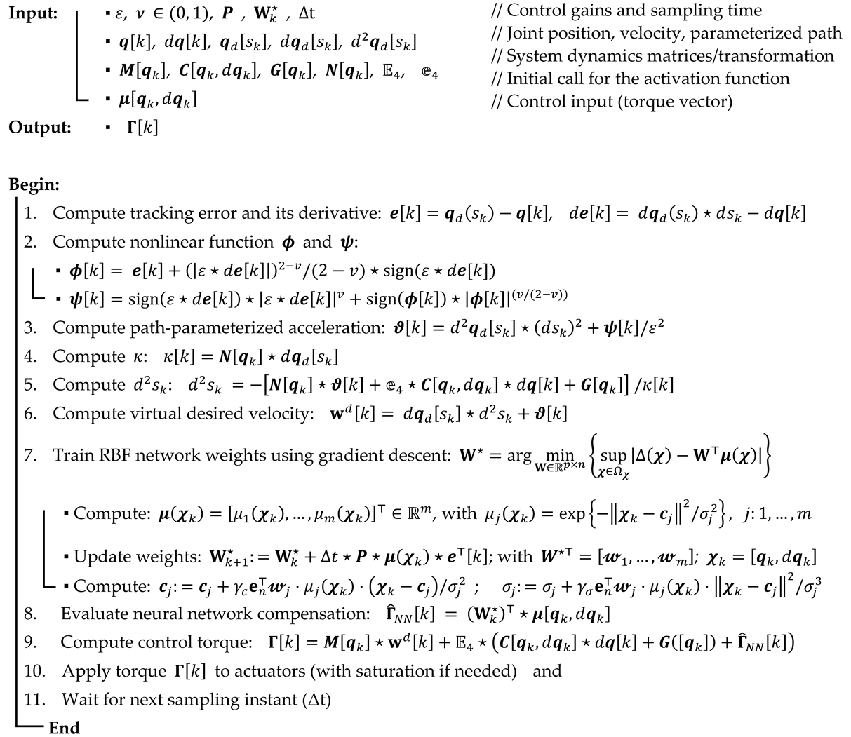
Algorithm 1: RBF Neural Network Training via Gradient Descent
Robotics 14 00084 i001

3.3. Adaptive Neural Network Control

Neural network-based adaptive control has emerged as a robust alternative to traditional model reference adaptive control (MRAC), especially for systems with high uncertainty and nonlinearities. Among neural models, radial basis function neural networks stand out for their universal approximation, rapid convergence, and structural simplicity (see Figure 13). Unlike MRAC, which adapts parameters via a reference model, RBFNNs use data-driven learning to directly approximate unknown dynamics, enhancing flexibility and real-time robustness. This contrast forms a foundation for advancing intelligent adaptive control in complex environments [26].
We employ a radial basis function neural network to approximate the unknown nonlinear functions and compensate for unmodeled dynamics and external disturbances in the bipedal locomotion control model. The system dynamics are expressed as M q q ¨ + C q , q ˙ q ˙ + G q = F + q , q ˙ , t . Here, . represents the lumped model uncertainties and external disturbances, which are approximated by the neural network x = W μ x + ϵ x , where ϵ x is the bounded error: ϵ x ϵ ¯ and
  • x = q , q ˙ R 2 n is the input vector (joint positions and velocities);
  • μ x R m is the RBF vector, defined by μ i x = exp x c i 2 / σ i 2 , i = 1 , , m ;
  • W R m × n is the ideal weight matrix.
The adaptive update law is derived using Lyapunov theory by W ^   = Γ W ϕ x e , where W ^ is the online estimated weight matrix, Γ W > 0 is the adaptation gain matrix, and e t = q t q d t is the velocity tracking error. To cancel uncertainty, the control input is given as F t = F 0 t W μ x , where the nonlinear dynamic inversion control is F 0 t = M q a 0 t + C q , q ˙ q ˙ + G q W μ q , q ˙ , with α 0 ,   1 being the fractional power and a 0 t = q ¨ d K 1 e α K 2 e ˙ . K 1   a n d   K 2 are gain matrices.
Theorem 3.
Under the control law  F t = F 0 t W μ x and adaptation mechanism, the tracking error e t = q t q d t converges to zero in finite time, and all signals in the closed-loop system remain bounded.
Proof. 
Define the Lyapunov Candidate Function V t = e t 2 + T r e W P 1 e W / 2 , with e W = W W . Taking the derivative and substituting the control law (with the Schwartz inequality) yields V ˙ t e K 1 e t α / 2 α e ˙ K 2 e ˙ t α + ε M . e ˙ t with 0 < α < 1 and x W μ x ε M . By choosing sufficiently large gains K 1   a n d   K 2 , the right-hand side becomes V ˙ t < c V t β . This differential inequality implies the finite-time convergence of e t to zero in the time bounded by t f V 0 β 1 / 1 β c . □

4. Stability and Control of RABBIT Robot

In this section, we propose a control law for the RABBIT robot and analytically demonstrate its asymptotic stability over a compound walking cycle consisting of simple-e-support phases separated by instantaneous impacts. Optimal trajectories are generated for the underactuated case. While the goal of walking control is to keep the robot within its viability space, designing a strategy around this concept is challenging due to the need to explore all possible biped movements. We therefore adopt a more restrictive approach focused on cyclic walking, where each step repeats identically with alternating leg roles. This periodic motion is represented in phase space by closed curves—known as limit cycles—where velocity is plotted against position (see Slotine and Li, 1991 [49]).

4.1. Nonlinear Decoupling Control

During flat-foot contact, a biped robot behaves as a fully actuated mechanical structure, allowing the use of classical control methods like PD, PID, or sliding mode. This section focuses on the computed torque control (input/output linearization), which uses the system’s dynamic model. With minimal parameterization, the stance-phase dynamics are expressed as follows [3,4,5,6,7,8]:
A 5 × 5 q q ¨ + C 5 × 5 q , q ˙ q ˙ + G 5 × 1 q = Γ 0
To track q d ( t ) , acceleration must be q ¨ = w d = q ¨ d + K v q ˙ d q ˙ + K p q d q , so
Γ   0 = A 5 × 5 q w d + C 5 × 5 q , q ˙ q ˙ + G 5 × 1 q
In a detailed manner, we can summarize the nonlinear decoupling control law (NDC) in
Γ = M 4 × 5 q w d + E 4 C 5 × 5 q , q ˙ q ˙ + G 5 × 1 q w h e r e w d = d q d   s   d s s ¨ + ϑ ϑ = d 2 q d   s   d s 2 s ˙ 2 + K v e ˙ + K p e e = q d q ; e ˙ = q ˙ d q ˙ κ = N 1 × 5 q d q d   s   d s A 5 × 5 q = M 4 × 5 q N 1 × 5 q M 4 × 5 q = E 4 A 5 × 5 q N 1 × 5 q = e 4 A 5 × 5 q E 4 = I 4 × 4 0 4 × 1 e 4 = 0 1 × 4 1 s ¨ = N 4 × 5 q ϑ + e 4 C 5 × 5 q , q ˙ q ˙ + G 5 × 1 q / κ
Chevallereau [19,29] defined the conditions for a joint path to yield stable, cyclic motion, with its attraction region bounded by angular momentum. Reaction force constraints (e.g., no take-off or slip) limit initial velocity. The proposed control law ensures convergence to a reference path in finite time, guaranteeing admissible motion.

4.2. Finite-Time Convergent Control

This type of control was proposed by Bhat and Bernstein in 1998 [28,29,50], and its basic idea is the choice of some gains such that the error will converges rapidly to zero. The high gains may directly affect motor torques, but they should be adjusted so that the maximum developed torques will never exceed 150 Nm. The acceleration of the robot has the form q ¨ = w d , which is
  q ¨ = q ¨ d + 1 ε 2 ψ = d q d d s s ¨ + ϑ s , s ˙ , q , q ˙ w h e r e ϑ = d 2 q d d s 2 s ˙ 2 + 1 ε 2 ψ ;   ψ = ψ 1 ψ 5
and the component ψ k is given by
ψ k = sign ε e ˙ q k ε e ˙ q k v + sign ϕ k ϕ k v 2 v ,   0 < v < 1 ϕ k = e q k + ε e ˙ q k 2 v 2 v sign ε e ˙ q k
When we replace acceleration q ¨ = w d in the 5 DOF model, we get the model Γ 0 = A 5 × 5 q w d + C 5 × 5 q , q ˙ q ˙ + G 5 × 1 q , and this can be written as
Γ 0 = A 5 × 5 q d q d d s s ¨ + ϑ + C 5 × 5 q , q ˙ q ˙ + G 5 × 1 q
If we multiply both sides by E 4 = I 4 × 4 0 4 × 1 , we get
Γ = M 4 × 5 q w d + C 4 × 5 q , q ˙ q ˙ + G 4 × 1 q
where M 4 × 5 q = E 4 A 5 × 5 ; C 4 × 5 q , q ˙ = E 4 C 5 × 5 q , q ˙ ; and G 4 × 1 q = E 4 G 5 × 1 q .
From the other side, if we multiply both sides by matrix e 4 = 0 1 × 4 1 , we get
N 1 × 5 q d q d d s s ¨ + ϑ + e 4 C 5 × 5 q , q ˙ q ˙ + G 5 × 1 q = 0
which implies that (i.e., with κ = N 1 × 5 q d q d   s / d s )
s ¨ = κ 1 N 1 × 5 q ϑ + e 4 C 5 × 5 q , q ˙ q ˙ + G 5 × 1 q
Finally, we summarize the finite-time convergent control (FTCC) in
Γ = M 4 × 5 q d q d d s s ¨ + ϑ + E 4 C 5 × 5 q , q ˙ q ˙ + G 5 × 1 q ϑ = d 2 q d d s 2 s ˙ 2 + ψ ε 2 ; κ = N 1 × 5 q d q d   s   d s   ψ = sign ε e ˙ ε e ˙ v + sign ϕ ϕ v 2 v ϕ = e + ε e ˙ 2 v 2 v sign ε e ˙     0 < v < 1   s ¨ = N 4 × 5 q ϑ + e 4 C 5 × 5 q , q ˙ q ˙ + G 5 × 1 q / κ    
Figure 14 illustrates the switching process between dynamic inversion and finite-time convergent control for a biped robot (the complete functional algorithm of this process is given in Appendix B). From the input state, joint variables and desired trajectories are computed. Based on the selected control type, the system derives the control law from the dynamic model to ensure accurate motion tracking.
Parameters v and ε are used to adjust the settling time of the controller. The key difference between the two control strategies lies in replacing K v e ˙ + K p e with ψ / ε 2 . The primary goal of walking robot control is to achieve cyclic movement, which is composed of several phases (such as the single-support phase, double-support phase, etc.) and impacts. Achieving this objective does not necessarily require the control to be stable during each independent phase, but rather, it demands convergence toward a limit cycle. In this context, the phase-plane representation of the nonlinear dynamic system serves as a valuable analytical tool. Starting from the initial conditions, the robot’s movement is traced in the phase plane, and the characteristics of the resulting curves are analyzed. Since robot walkers have more than two states, each joint’s movement is represented in its own phase plane and plotted according to the joint position. The robot’s movement corresponds to the succession of these differential phases (see Figure 15), and cyclic movement forms a closed curve in each phase plane.
If this closed cycle (see Figure 15) is isolated, it represents a limit cycle, which can be stable, unstable, or semi-stable. Movements near the limit cycle may converge toward it. Henri Poincaré developed a technique to analyze dynamic system stability by creating a hyper-surface of dimension n 1 , transversal to the limit cycle. The flow’s intersection with this hyper-surface leads to the Poincaré return map. The control law uses computed torque, a standard method in robotics, with a slight modification to ensure finite-time convergence to the desired path. The finite-time feedback control proposed in [17,18,19,20,21,22,23] and [31] is employed. Joint-tracking errors are defined relative to trajectories satisfying the desired path as follows: e t = q d s t q t , e ˙ t = d q d / d s s ˙ q ˙ t . The desired behavior of the configuration variables in the closed loop is given by q ¨ = q ¨ d + ψ / ε 2 , where ψ q ,   q ˙ ,   s ,   s ˙ from [25,28] is the term that ensures q t q d s t     0 in finite time. In fact, the settling time can be chosen to be shorter than the time duration of a step.

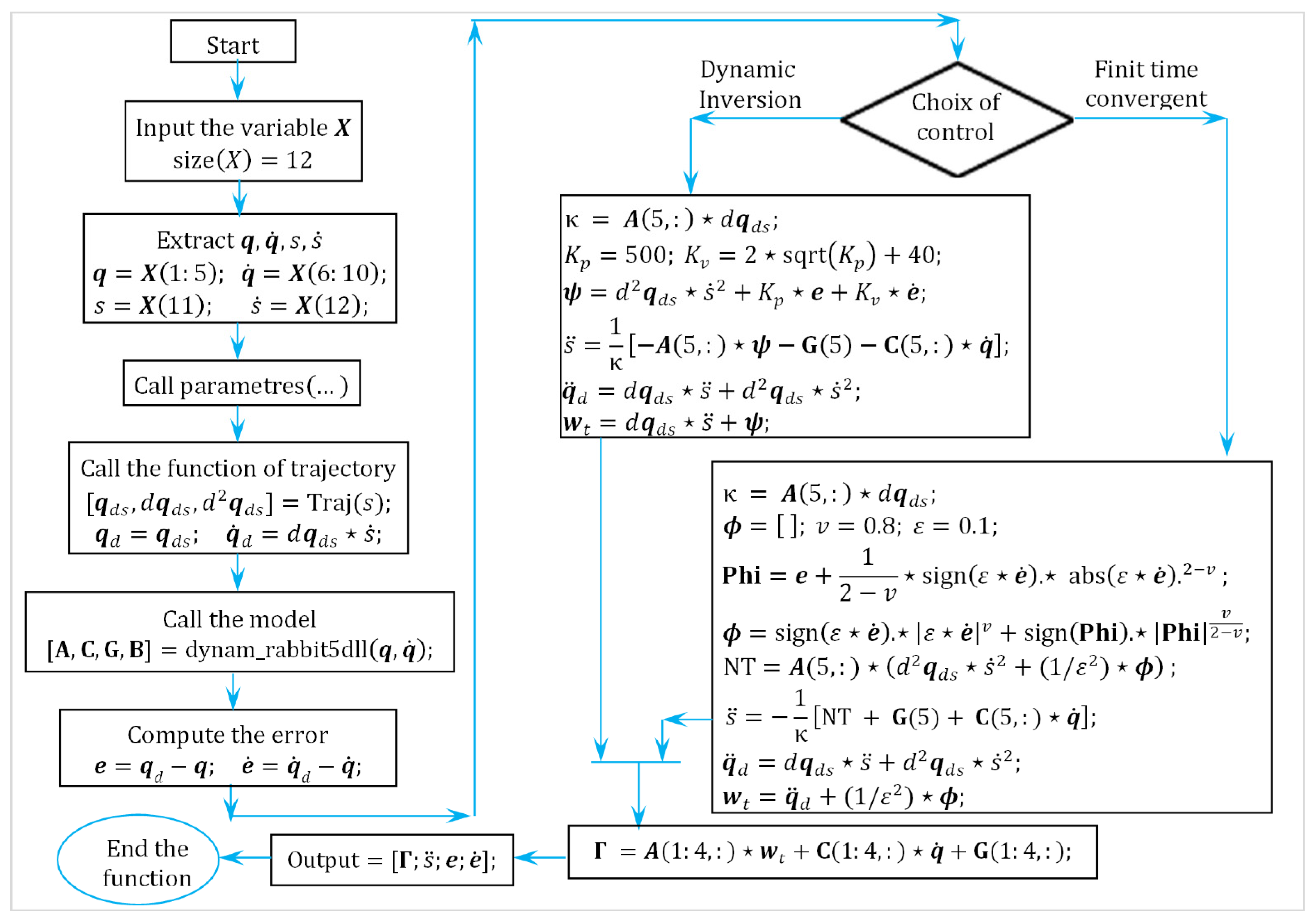
4.3. The Proposed Adaptive Finite-Time Convergent Control

The previous approach relies on the exact cancelation of system nonlinearities. However, uncertainties in parameter values, computational round-off errors, and the computational burden of modeling complex systems make exact cancelation impractical. To address this, it is often necessary to simplify the equations of motion by neglecting certain terms, enabling the faster computation of the control law. Thus, the adaptive nonlinear control law is more realistically expressed as a linear combination of two control signals: Γ t = Γ i d e a l t + Γ a d a p t i v e t , where Γ a d a p t i v e t = K ϕ t μ q and Γ i d e a l t = M 4 × 5 q w d t + E 4 C 5 × 5 q , q ˙ q ˙ + G 5 × 1 q . The vector q t represents the state of the controlled system, while μ q encapsulates the disturbance model features. K ϕ t is an adaptive weight vector for the disturbance model. The controller calculates the error e t between the system’s state and the reference model’s state. This error is then used to adapt the value of K ϕ t in real time. The adaptive controller estimates the model’s uncertainty dynamically and generates an adaptive control action Γ a d a p t i v e t that cancels out the uncertainty, thereby restoring the nominal system for the baseline controller. The adaptive control term models system uncertainty as follows: Γ a d a p t i v e = K ϕ μ q , where K ϕ t = E 4 W T t ; W t contains the network weights adjusted by the controller. μ q is the feature vector of the uncertainty model. For nonlinear or unknown disturbance models, radial basis functions (RBFs) with Gaussian kernels are employed. In adaptive learning control, the RBF kernel is commonly used in kernel-based algorithms. Equation (32) defines the adaptive control law as the sum of an ideal component and an adaptive term that compensates for system uncertainties.
Γ = M 4 × 5 q w d + E 4 C 5 × 5 q , q ˙ q ˙ + G 5 × 1 q + W μ w d = d q d s   d s s ¨ + ϑ s , s ˙ , q , q ˙   ϑ = d 2 q d d s 2 s ˙ 2 + ψ ε 2 ; κ = N 1 × 5 q d q d   s   d s   ψ = sign ε e ˙ ε e ˙ v + sign ϕ ϕ v 2 v   ϕ = e + ε e ˙ 2 v 2 v sign ε e ˙ 0 < v < 1   s ¨ = N 4 × 5 q ϑ + e 4 C 5 × 5 q , q ˙ q ˙ + G 5 × 1 q / κ   d W d t = P μ q d s q ; μ = v e c t o r   o f   b a s i s   f u n c t i o n s
An adaptive radial basis function neural network is employed in the design of the regulator, which consists of two layers: the input-hidden layer and the output layer. The weight matrix W plays a crucial role here, as sensory feedback is integrated into it. The update learning rule for W is given by the following update rule: W ˙ t = P μ e t , where μ (i.e., μ i = exp γ x x i 2 ) is the vector of radial basis functions, and γ is the learning rate. The matrix P is positive definite. The unknown variations of Δ t = W μ are approximated by a neural network (such as RBFNN or multilayer perceptron), where W denotes the matrix of unknown weights to be identified. This formulation can represent various feedforward and recurrent neural networks. Given the universal approximation property of neural networks, we have Δ ^ t = W μ + ε , where W is the optimal (unknown) weight, and ε represents the bounded approximation error ( ε ε M ).
Condition of convergence and existence of cyclic motion: To establish convergence and the existence of cyclic motion in our planar biped, we examine the single-support phase using the selected coordinate system. The derivative E k / q ˙ 5 represents the angular momentum σ of the biped about the stance leg tip S i . This quantity is given by σ = E k / q ˙ 5 = N q c q ˙ , where N q c corresponds to the fifth row of the matrix A 5 q c + m f i q / q f i q / q . Furthermore, the derivative of the potential energy with respect to q 5 is E p / q 5 = m g x S i x g . Accordingly, the fifth equation of the dynamic model during the single-support phase can be expressed in the following simple form:
σ ˙ t = N q c q ¨ t + q ˙ t N q c / q q ˙ t = m g x S i t x g t
We define the desired configuration of the biped as q d t = q r s t , where q r s is a prescribed vector function parameterized by the scalar s . If κ = N q c q r / s 0 , then the proposed control law guarantees the convergence of q t to q r s t in finite time, which can be made shorter than single-step durations [19,20,50]. In the absence of initial errors, the trajectory q r s t is tracked exactly. The evolution of s t is derived from s ¨ t , provided that the initial conditions s 0 and s ˙ 0 are known. We set s 0 = 0 and select s ˙ 0 to minimize the initial joint velocity error.
ϵ = q ˙ 0 q ˙ r 0 2 = q ˙ 0 q r s 0 / s s ˙ 0 2
Thus, s ˙ 0 is such that ϵ / s ˙ 0 = 0 . We obtain
s ˙ 0 = q ˙ T 0 q r s 0 / s / q r s 0 / s T q r s 0 / s
From the equation for s ¨ t , it follows that a singularity arises in the proposed control law if κ = N q c q r / s = 0 . For the reference trajectory q s = q d s , we define the function f s = N q r s q s / s . Although N depends only on the first four components of q r s , we retain notation N q r s for clarity. If f s remains sufficiently bounded away from zero along the reference path and the tracking error stays small, singularities are avoided.
The objective is to develop a control strategy that guarantees the stable periodic motion of the biped robot. The control input s ¨ t ensures finite-time convergence to a reference trajectory q d t = q r s t , with the convergence time chosen to be shorter than the one-step duration. Consequently, from the second step onward, the biped accurately tracks the reference path. In this framework, the 5 DOF biped model is reduced to a 1 DOF model in terms of s t , based on the prescribed reference. This reduced model resembles an inverted pendulum, and its analysis focuses on the existence and uniqueness conditions for admissible cyclic trajectories.
During the single-support phase, the biped behaves as an underactuated system, meaning that it cannot arbitrarily track a desired trajectory q d t . A trajectory q r s t is termed an admissible reference motion if it satisfies the system’s dynamics. The analysis of angular momentum σ is sufficient to determine the evolution of the scalar parameter s , from which the full motion of the robot can be derived. Since σ is linear with respect to the velocity vector q ˙ t and given that the velocity along the reference motion is proportional to s ˙ , the angular momentum can be expressed as σ = f s s ˙ . The scalar function f s depends on q r s and the physical parameters of the biped. Assuming f s 0 over the interval 0 s 1 , the function is either strictly positive or strictly negative. In the remainder of this discussion, we assume f s > 0 . It follows that s ˙ = σ / f s . If the reference path q r s is known, then the horizontal position x g of the center of mass can also be expressed as a function of s , denoted as x g = x g s . In this case, the derivative of the angular momentum becomes σ ˙ = m g x g s x S i . Under a prescribed joint trajectory, the equations for σ ˙ t and s ˙ t together form a reduced-order model that captures the admissible dynamics. Given the initial values for σ and s , the functions   σ t and s t can be uniquely determined. The second system, which is composed of two subsystems s ˙ t = σ / f s ; σ ˙ t = m g x g s x S i is analogous to the classical equation of motion for a physical pendulum with a single degree of freedom [19,51]. As such, it admits an integral of motion similar to the energy integral of pendulum dynamics. Specifically, the system has conserved quantity σ 2 t ϕ s = c n s t , where ϕ s is a scalar potential function associated with the configuration-dependent gravitational term:
ϕ s = 2 m g k + s x g ξ x S i f ξ d ξ ; k   d e n o t e   t h e   k t h   s t e p
Using the expression σ = f s s ˙ , the integral of motion σ 2 t ϕ s = c n s t can be rewritten as f 2 s s ˙ 2 s ϕ s = c o n s t a n t or, equivalently, f 2 s s ˙ 2 s f 2 k + s ˙ 2 k + = ϕ s . The functions f s and ϕ s can be computed once the reference trajectory q r s is specified. These functions are periodic with period 1, so the robot’s behavior can be analyzed within the interval of 0 s 1 , corresponding to a single step. For human walking, the abscissa x g of the center of mass increases over time. To mimic this behavior, we choose q r s such that x g increases with s on the interval [ 0 ,   1 ] . The single-support phase starts when x g < x S i and ends when x g > x S i . The potential function ϕ s reaches a negative minimum value ϕ m s = min 0 < < 1 ϕ s = ϕ s g at s = s g , where x g s g = x S i . After this point, x g > x S i and ϕ s increase strictly monotonically. These results are summarized in the following theorem.
Theorem 4.
The path  q r s with   k < s < k + 1 can be achieved by the biped if and only if   σ ˙ k + > ϕ m or s ˙ k + > ϕ m / f 0 + .
A cyclic admissible reference motion is defined by a periodic evolution of the angular momentum σ or, equivalently, by a periodic evolution of the scalar velocity s ˙ , denoted as s ˙ c . All admissible reference motions satisfy the energy-like relation σ 2 t ϕ s = c n s t and are fully characterized by the definition of ϕ s . Therefore, a cyclic admissible reference motion exists i f f there exists an initial angular momentum σ k + such that σ k + 1 + = σ k + or, equivalently, if and only if there exists an initial velocity s ˙ k , denoted as s ˙ c k , such that the time-increasing s ( t ) satisfies s ˙ k + 1 = s ˙ k = s ˙ c k = s ˙ c 0 . Under these conditions, the biped’s states are identical at the beginning of steps k and k + 1 (except for the role-swapping of the legs). Given the periodic nature of f s and ϕ s , the following must hold: f 2 1 s ˙ c 2 0 f 2 0 + s ˙ c 2 0 = ϕ 1 . Analyzing this equation, we conclude the following necessary condition for the existence of a cyclic admissible reference motion:
  • If f 0 + = f 1 and ϕ 1 = 0 , any initial value s ˙ k > s ˙ m yields cyclic ref-motion.
  • If f 0 + = f 1 and ϕ 1 0 or if values ϕ 1 and f 2 1 f 2 0 + have different signs, then there is no cyclic reference motion.
  • The previous equation has a unique solution s ˙ c 0 = ϕ 1 / f 2 1 f 2 0 + 1 / 2 if and only if values ϕ 1 and f 2 1 f 2 0 + have the same sign.
Using equation of s ˙ c 0 , the next theorem can be formulated.
Theorem 5.
A unique cyclic reference motion exists if and only if the following is satisfied:   ϕ 1 / f 2 1 f 2 0 + + ϕ m / f 2 0 + > 0 . The initial cyclic velocity for one step is defined by equation   s ˙ c 0 = ϕ 1 / f 2 1 f 2 0 + 1 / 2 .
We assume the existence of a unique cyclic admissible reference motion and that the initial velocity s ˙ is sufficiently large to ensure a monotonic evolution of the parameter s t . We define the relative velocity error, or “velocity diff”, between the actual velocity s ˙ s and the nominal cyclic velocity s ˙ c s by the expression e s = s ˙ s s ˙ c s / s ˙ c s . The biped motion converges to the cyclic reference if and only if e s converges to zero, i.e., if the actual velocity s ˙ s converges to the nominal cyclic velocity s ˙ c s . Using the energy relation derived previously, e s can be explicitly expressed as a function of the initial error e k for k < s < k + 1 , yielding the following equation:
  e s = 1 + e k e k + 2 f 2 0 + s ˙ c 2 0 f 2 0 + s ˙ c 2 0 + ϕ s 1 / 2 1
The expression of the error function e ( s ) includes a square root and is well-defined only for positive arguments. This imposes the following condition on the initial error e ( k ) : e k > ϕ m / f 0 + s ˙ c 0 . This inequality is equivalent to a lower bound on the initial velocity: s ˙ k + > ϕ m / f 0 + . This condition guarantees that the argument under the square root in e s remains strictly positive, allowing a valid evaluation of the velocity error over the interval. The evolution of the velocity difference e s over a single step can be directly deduced from the evolution of the function ϕ s . While the function ϕ s is cyclic, it is not continuous at the step boundary s = k . Therefore, Equation (37) for e s is only valid within a single-step interval k < s < k + 1 . However, the velocity difference e s itself remains continuous at s = k because both s ˙ s and s ˙ c s are continuous at that point. This allows a consistent evaluation of e k + 1 based on e k . Using the earlier relation, f 2 1 s ˙ c 2 0 f 2 0 + s ˙ c 2 0 = ϕ 1 , we derive an iterative formula for the evolution of e k from one step to the next:
e k + 1 = 1 + e k e k + 2 f 0 + f 1 2 1 / 2 1
Theorem 6.
(Condition of Convergence): The admissible reference motion converges towards the cyclic admissible reference motion if and only if  s ˙ 0 > ϕ m / f 0 + and   f 0 + > f 1 (or equivalently   ϕ 1 > 0 ).
Proof. 
With k < s < k + 1 , if k , then error function e s 0 is uniform for any s if and only if e k 0 when k because e s is defined by the equation of e s , and the function f 2 0 + s ˙ c 2 0 / f 2 0 + s ˙ c 2 0 + ϕ s is cyclic and bounded. Thus, to prove that biped motion converges to the cyclic admissible reference motion, it is necessary and sufficient to prove the convergence of e s towards 0 when k . If f 0 + < f 1 , then using the equation of error e k + 1 and inequality f s > 0 , we can deduce that e k + 1 f 0 + / f 1 . e k , and we can conclude that   e k 0 when k . It follows from the equation of e k + 1 that if f 0 + = f 1 , then e k + 1 = e k . If f 0 + > f 1 , then e k + 1 f 0 + / f 1 . e k , and there is no convergence. The condition s ˙ 0 > ϕ m / f 0 + ensures that s t is an increasing function during the first step. If f 0 + < f 1 , the condition s ˙ k > ϕ m / f 0 + will be satisfied for all k , and the function s t increases for all steps. □
The convergence of the admissible reference motion can also be shown using a section of the Poincare map as in [17,19,25]. The equation of e k + 1 easily allows the use of e k + 1 as a function of e k . Combining Theorems 4–6, the next corollary can be deduced.
Corollary 1.
The admissible reference cyclic motion is orbitally asymptotically stable if and only if the reference joint path is such that
f 0 + < f 1 ,   ϕ 1 f 2 0 + + ϕ m f 2 1 f 2 0 + > 0
According to the above theorems and this corollary, the conditions for the existence and convergence of cyclic motion are defined by inequalities. Therefore, the proposed control strategy inherently includes robustness. Despite tracking or modeling errors, the robot’s behavior will converge to cyclic motion provided that the reference path is suitable (i.e., it satisfies the inequalities with some margin). In the presence of modeling errors, the resulting cycle may deviate slightly from the predicted cycle, but stable walking will still be achieved, as demonstrated in the experimental results.
Discrete implementation of the proposed algorithm: Although the control algorithm is formulated in continuous time, its real-world implementation requires discretization due to the sampled nature of digital platforms like dSPACE DS1103, which features a 400 MHz PowerPC 604e DSP. The algorithm was executed with a fixed sampling period of Δt = 1.5 ms (667 Hz). Using a zero-order hold (ZOH), control inputs are assumed constant between samples, and all states are updated at each discrete time step:
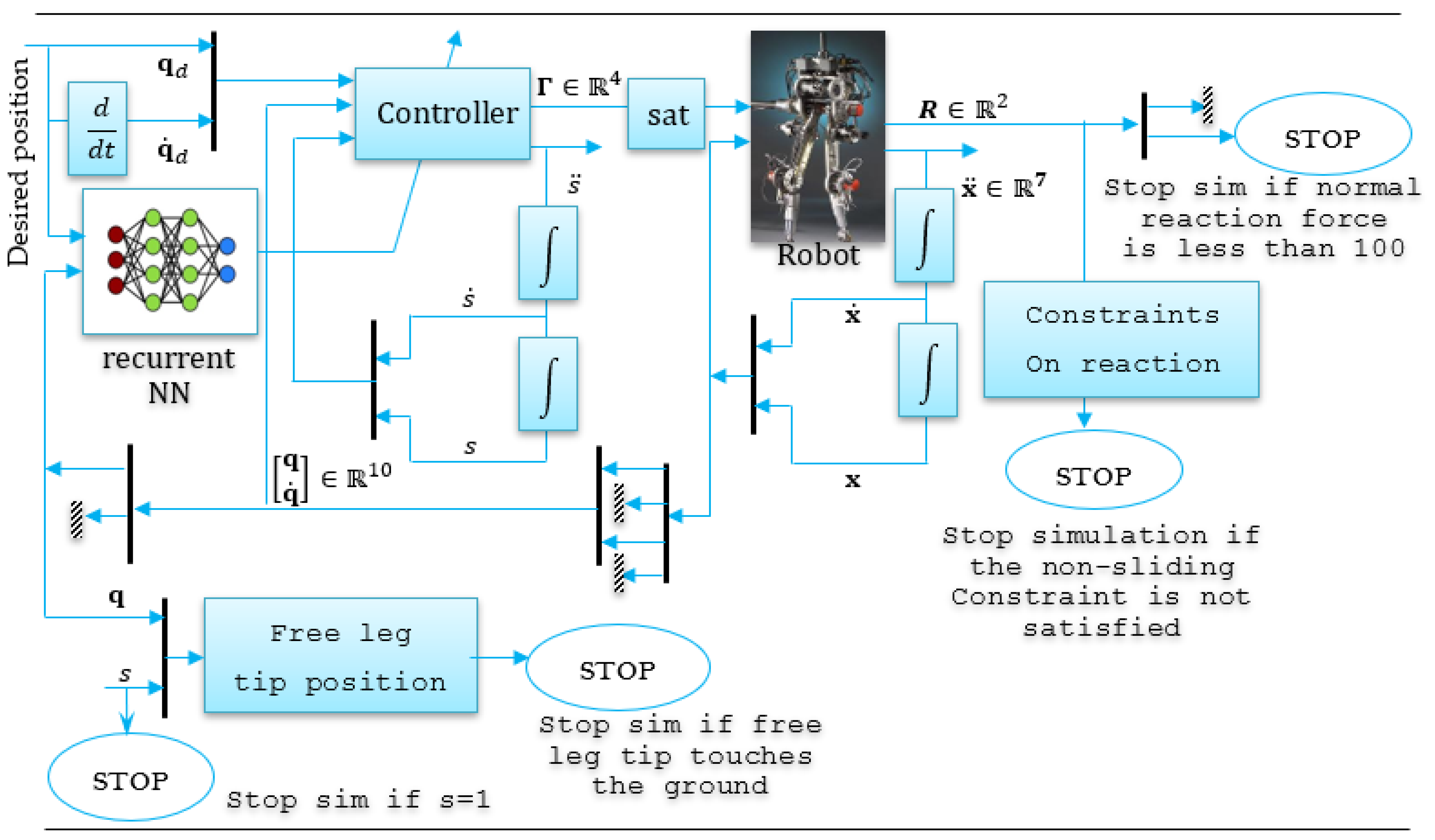
  • Sampling and Discretization Framework: The control algorithm was implemented on a real-time platform with a fixed sampling rate of Δ t = 1.5   m s   ( f r e q = 667   H z ) . To discretize the continuous-time controller, we adopted zero-order hold (ZOH) assumptions, which consider control inputs constant between samples. The state updates are computed at each sampling instant.
  • Discretization of the Control Law: The control law includes the following:
    • An FTC correction term Γ F T C t (including the dynamic inversion);
    • An adaptive RBF neural network compensation term Γ N N t
Each term is computed at sampling t k = k . t as Γ k = Γ F T C k + E 4 Γ N N k , where the following is the case:
  • Γ F T C k includes fractional or high-gain error terms computed via FTCC logic;
  • Γ N N k = W ^ k μ q k , q ˙ k .
Care is taken to handle potential high-gain effects to avoid numerical instability.
3.
Numerical Differentiation: Velocity q ˙ and acceleration q ¨ are approximated by q ˙ [ k ] q k q k 1 / Δ t and q ¨ k q ˙ k q ˙ k 1 / Δ t . Given the sensitivity of numerical differentiation to noise, digital filters (e.g., low-pass filters, Kalman filter, or Savitzky–Golay filter) are employed to smooth the signals, ensuring accurate derivative estimation without amplifying measurement noise.
4.
Neural Network Online Update: The RBF neural network is trained online using discrete adaptation: W ^ k + 1 = W ^ k + Δ t P μ k e k . This ensures real-time learning while keeping the update rate within the system’s computational limits.
5.
Real-Time Execution: The full control loop is executed at each sampling instant on the dSPACE DS1103 platform. The timing constraints ( 1.5   m s were met through:
  • Efficient MATLAB/Simulink code generation;
  • Pre-computation and lookup tables for RBF activations;
  • Optimization of matrix operations and control scheduling.
6.
Validation and Testing: Discrete implementation was tested via the following:
  • Hardware-in-the-loop (HIL) simulation;
  • Real-time experiments under various scenarios.
The scenarios included actuator limits, external disturbances, inertia variations, and sensor noise. Feedback was provided by high-resolution encoders (C4 and CHM 506) fil-tered for accuracy. Robustness to mechanical imperfections and terrain variation was handled through adaptive compensation/safety mechanisms (e.g., emergency stops).
7.
Performance Preservation: The discretized control law successfully preserved key properties of the original continuous-time formulation, including the following:
  • FTC convergence through gain-tuned discretization framework;
  • Robustness to uncertainties maintained via filtering and adaptive NN updates;
  • Bounded control effort and tracking ensured through careful discretization and real-time computation strategies.
The control loop ran reliably at a 1.5 ms cycle despite hardware constraints like backlash, compliance, and actuator saturation. The discretized control law preserved finite-time convergence, robustness through filtering and adaptation, and bounded control efforts, enabling stable and accurate bipedal locomotion in real-world tests.
Presented below (in Algorithm 2) is a formal pseudocode of the complete implemented control algorithm.
Algorithm 2: The complete algorithm of the implemented discrete control law
Robotics 14 00084 i002

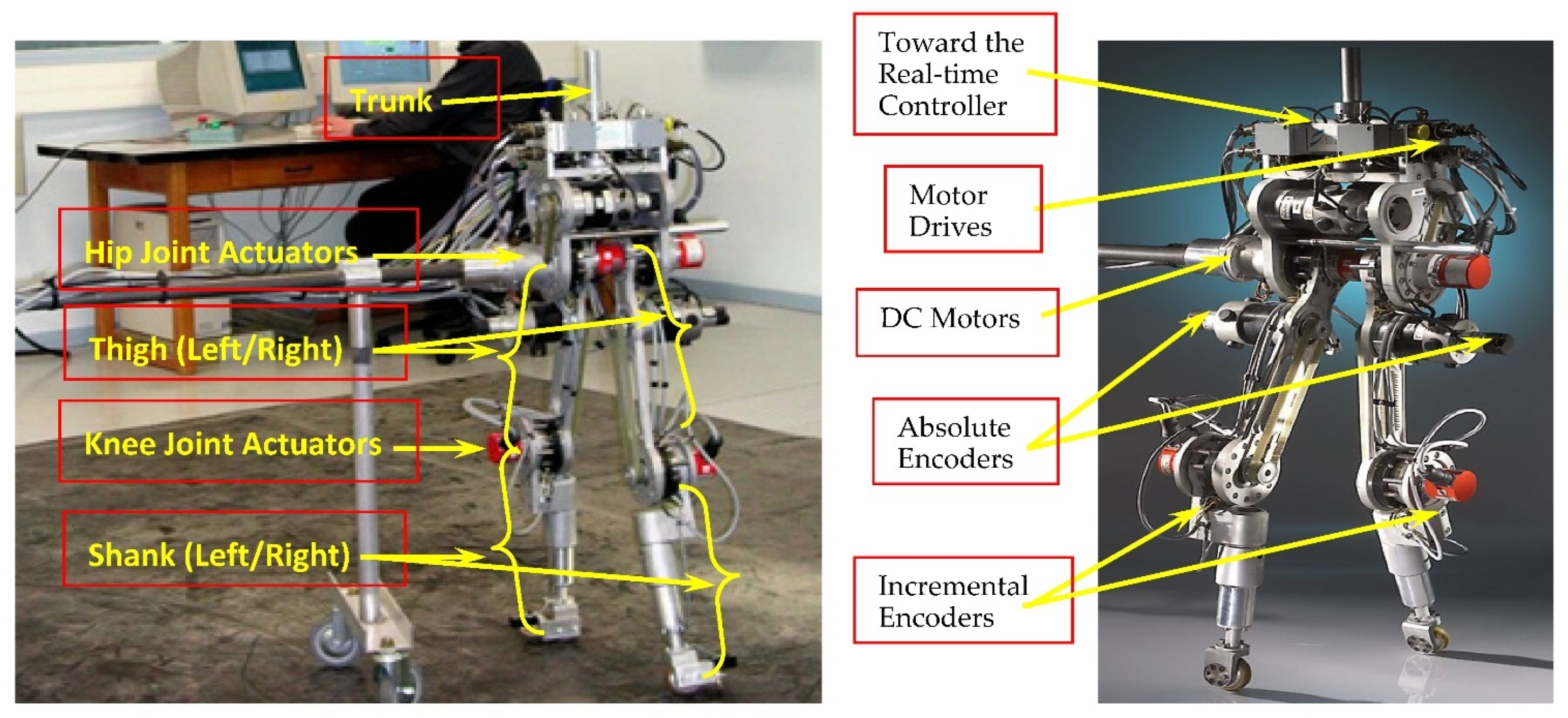
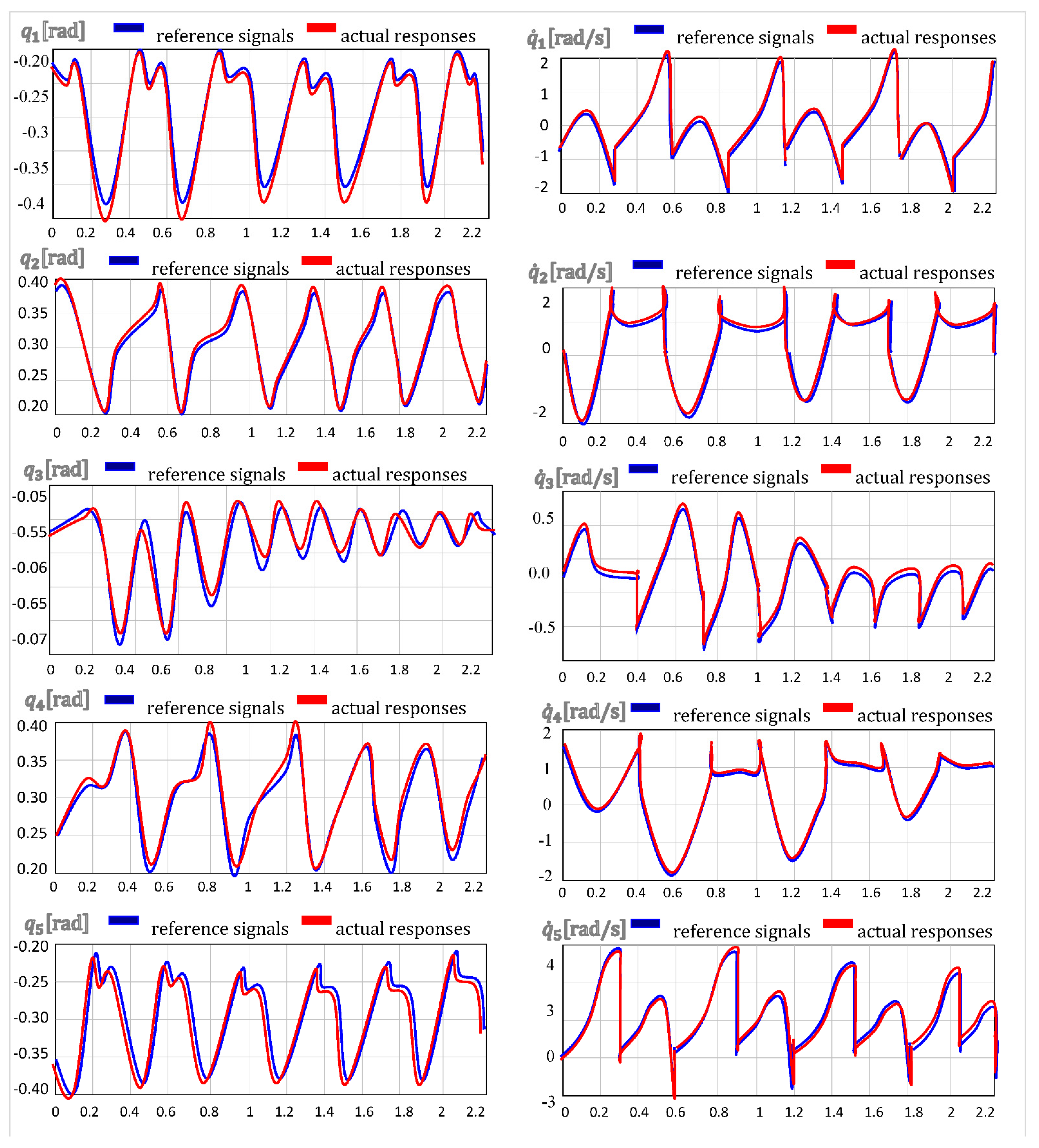
5. Experimental Results of the RABBIT Robot

To implement the proposed control algorithm, the dSPACE DS1103 system was employed as the real-time control platform. This system enables the automatic generation and cross-compilation of SIMULINK diagrams into run-time software for its 400 MHz PowerPC 604e DSP, allowing controller development using a high-level language. The DS1103 also integrates essential functionalities—including low-level computations, digital-to-analog and analog-to-digital conversions, and a user interface—within a single package. This eliminates the need for low-level I/O programming and significantly streamlines the debugging process. Control computations were executed with a sampling period of 1.5 ms (667 Hz). The used components are given in Table 2.
Modeling errors are an inherent challenge in any control strategy. Given the complexity of the RABBIT mechanism (Figure 16), various factors contribute to discrepancies between the idealized dynamics and the actual system, leading to modeling errors:
  • Friction in the motor–belt–gear assemblies and at the tower’s universal joint;
  • Unmodeled flex dynamics due to cabling, gear torsion, and deformation;
  • Inaccuracies due to poor estimates of link inertias + dSPACE + power electronics;
  • Digital implementation limitations (e.g., sampling, quantization);
  • Non-rigid impacts due to compliance at the end of the leg, etc.
In addition to control design and modeling, the robot’s mechanical structure contributes to robustness. Several imperfections and structural tolerances, though not explicitly included in the model, play a practical role in ensuring stable locomotion:
  • Joint Backlash Tolerance: ±0.8° due to slack and gear tolerances.
  • Linkage Compliance: Up to 1.2 mm deflection under peak load.
  • Assembly Misalignments: Errors up to ±0.5 mm between joint axes.
  • Flexibility: ~2–3 mm compliance in the foot–ground interface, damping vibrations.
  • Unmodeled Dynamics: 4–6% damping from residual friction stabilizes oscillations.
These mechanical flexibilities, although not accounted for in the L a g r a n g i a n model, act as passive stabilizers. They absorb impact shocks, reduce vibration transmission, and help maintain the integrity of the gait cycle under experimental conditions.
The RABBIT robot is the result of a collaborative effort among seven French laboratories (IRCCYN Nantes, LAG Grenoble, LMS Poitiers, LVR Bourges, LGIPM Metz, LRV Versailles, and LIRMM Montpellier), developed under the CNRS ROBEA project focused on the control of bipedal robots for walking and running. As illustrated in Figure 16, the robot consists of two legs and a trunk but lacks feet. Its joints are positioned at the hips and knees, and it is equipped with four actuators—one at each knee and one at each hip. The physical properties of RABBIT, including limb masses and lengths, are detailed in Table 1. Movement is constrained to the sagittal plane through a radial bar linked to a central column, which guides the robot’s forward motion along a circular path. RABBIT represents a minimal bipedal system capable of producing both walking and running gaits. Below is an overall scheme for the controlled RABBIT robot simulator (Figure 17).
To provide clarity and ensure the reproducibility of this experimental study, we list the fourteen functions utilized throughout the implementation in the following table.
•The 1  function:  Main ProgramThe primary script coordinating the simulation.
•The 2  function:  robot_parametresDefines the physical parameters of the robot.
•The 3  function:  [Out1] = dm7dof (Entree1)Computes the dynamic equations of the 7 DOF robot.
•The 4  function:  [Out] = reaction_forcesde (R1)Calculates the ground reaction forces.
•The 5  function:  [qp,Ir] = impact (qf,qpf)Models the impact phase/computes post-impact velocities.
•The 6  function:  [A,Ac1,Ac2] = dynam_impact (qf)Computes dynamic matrices related to the impact.
•The 7  function:  [qd_s,dqd_s,ddqd_s] = Traj (s)Generates the desired trajectory.
•The 8  function:  stick_inf (x)
Displays or manages the stick-figure representation.
•The 9  function:  [Out] = pos_swing_leg (Entree)Computes the position of the swing leg.
•The 10 function:  [Out] = discrete_control _law (Entree)
Implements the discrete-time control law.
•The 11 function:  [A,C,G,B,Ac1,hxs] = dyn_7dof_rabbit (q,dq)Returns the full dynamic model of the 7 DOF RABBIT.
•The 12 function:  [A,C,G,B] = dynam_5dof_rabbit (q,dq)Provides the reduced 5 DOF dynamic model.
•The 13 function:  [dqp,F] = post_impact_dynamics (q,dqm)Calculates post-impact dynamics.
•The 14 function:  dess (tout,ERR,ERRP,qp,qpp,R,pos_p,Gama)Handles the graphical visualization of the results.
Challenges in early model development and solutions: During development, challenges included modeling complex nonlinear dynamics, ensuring controller stability under uncertainties, and managing hardware limitations and disturbances. These issues were addressed through advanced simulation, adaptive and robust control, noise filtering, phased testing, and safety protocols. The proposed control system utilizes high-performance hardware, notably a dSPACE DS1103 controller with a 400 MHz PowerPC 604e DSP capable of executing complex algorithms—including neural updates and filtering—within a 1.5 ms sampling period. Real-time performance is maintained via optimized codes, pre-computation, and efficient matrix operations. The system employs high-torque DC motors (RS420J) driven by RS420 RTS10/20-60 current drives, which enable precise control but are limited by thermal and current constraints that risk saturation under high loads. Motion transmission through HFUS-2UH gear reducers (1/50) introduces compliance, backlash, and delay, affecting accuracy. Position feedback from C4 incremental encoders (250 counts/rev) and CHM 506 P426R absolute encoders (8192 counts/rev) provides high resolutions, necessitating filtering methods like Kalman filters to mitigate noise. Mechanical imperfections and backlash induce nonlinearities that require robust control strategies, while external disturbances and terrain variability challenge stability and are managed adaptively. Safety measures include soft limits, emergency stops, and fault detection. The hardware’s operational limits highlight the importance of optimized and adaptive control to ensure reliable bipedal locomotion. Table 3 summarizes these issues and their corresponding solutions.
First experimental scenario: The theoretical results previously established were evaluated using a closed-loop test of the locomotion system. The experiment (Figure 18) involved implementing the dynamic control law with parameters ε = 0.1   a n d   ν = 0.8 . The system was initiated on a cyclic trajectory under ideal conditions without introducing model errors. The results demonstrate that the proposed control law effectively drives the robot’s states to accurately track the reference trajectory.
Figure 18 illustrates the robot’s behavior during the first five steps under the proposed control law, showing a transition from the initial state to a stable, symmetric gait with constant forward velocity per step. The close alignment between the reference and actual responses highlights the excellent trajectory tracking performance of the implemented control system. Regular, repeating patterns in the joint variable evolution and near-zero tracking errors confirm orbital stability and indicate that cyclic walking motion has been achieved. Sharp transitions in velocity profile q ˙ correspond to impact events, where the swing leg contacts the ground and role switching occurs, further confirming the controller’s effectiveness in handling the hybrid dynamics of bipedal locomotion. Figure 19 shows motor controls remaining well below the 30 N limit during a cyclic step. It also illustrates joint positions and velocities in the phase plane, confirming that the control law maintains the robot on its cyclic trajectory. While tracking errors exist, they remain cyclic. Ground reaction forces consistently point upward, ensuring contact constraint compliance. The phase-plane evolution of a joint variable reveals motion convergence and impact moments. The stabilization of q 1 , q 2 , and q 3 relative to the desired limit cycle demonstrates rapid control input convergence and diminishing tracking errors, restoring cyclic motion within a few steps.
The proposed method offers a globally convergent adaptive controller without relying on local linearization, time-invariance, or decoupled dynamics. It inverts the estimated inertia matrix and numerically differentiates joint velocities. With adaptation slower than the control bandwidth, the controller—validated on the underactuated RABBIT biped in single support—achieves geometric tracking that adapts to gravity and reference sequences (Figure 20). It converges to a stable limit cycle despite initial mismatches, model errors, or disturbances.
Second experimental scenario (Robustness Testing 1): The robustness of the proposed control law is assessed by introducing intentional parameter uncertainties (Figure 21). The inverse dynamics use online adaptation, while the direct dynamics are deliberately perturbed to reflect modeling errors, including mass and inertia increases ( + 20 % for thighs, + 30 % for tibias, + 100 % for the trunk, and + 30 % for trunk inertia) and a horizontal force of 350   N applied to the center of mass during 1.2   s < t < 4.4   s .
An experimental evaluation (see Figure 21) was carried out for five steps, assuming no modeling error at the initial step. The state of the robot was initialized on the periodic orbit (see Figure 21a). From these results, we notice that, starting on the cyclic trajectory, all constraints are satisfied, and trajectory tracking is perfect, but the initial speed of the curvilinear abscissa is limited by a maximum value, beyond which the robot may violate constraints during the step (Figure 21b,c). Convergence toward a periodic motion was obtained for each of the five joints of the robot (Figure 21d). For this value, the torques are at the limit of the value 150 Nm. The results presented correspond to five steps, using the same control parameters ( ε = 0.1 and ν = 0.8 ).
Third experimental scenario (Robustness Testing 2): This experimental scenario investigates the robustness of the control strategy under combined structural and parametric uncertainties. Specifically, the contact model was structurally modified, and mass/inertia discrepancies of ±20% were introduced between the control model and the real model while maintaining symmetry between the legs. These perturbations inherently cause deviations in the robot’s state during ground contact. Additionally, the mismatch between the flight-phase controller and the real model prevents the precise conservation of angular momentum upon landing. To further reflect realistic physical constraints, a torque saturation of ±150 Nm was enforced, consistent with the actuator limits of the RABBIT platform. The corresponding results are illustrated in Figure 22.
Figure 22 shows the time evolution of the joint trajectory q i t (top subplots), along with their corresponding tracking error e i t = q i t q i r e f t (bottom subplots), for all four joints of the biped robot over a time window of 35 to 38 s. The reference trajectories (dashed lines) are compared against the actual responses (solid blue lines), and the performance of the proposed neural adaptive controller can be evaluated accordingly. The plots clearly demonstrate that the actual joint trajectories closely follow the desired periodic reference signals, with minimal phase lag or amplitude deviation. The corresponding tracking errors remain bounded and within a narrow range (less than ±0.04 rad), reflecting high precision and the robustness of the controller even under disturbances or uncertainties. These results confirm that the controller ensures accurate trajectory tracking, stability, and synchronization across all joints. The periodic nature of the motion and the small tracking errors indicate convergence toward a stable limit cycle, validating the controller’s effectiveness in maintaining coordinated bipedal locomotion. The control behavior and phase-plane convergence are shown in Figure 23.
Figure 23 present the phase-plane trajectories of the configuration variables, clearly illustrating convergence to a stable limit cycle. Upon touchdown, the leg roles switch, replicating the behavior observed under the rigid contact model. At the beginning of the stance phase, the impact causes an abrupt change in the robot’s velocities, which, at that instant, still reflect their flight-phase values. Since the initial conditions are taken from the periodic orbit of the rigid contact model and no parametric modeling errors are introduced, flight-phase perturbations remain minimal. The results confirm the existence of a stable periodic gait. The obtained responses further demonstrate that the proposed neural adaptive controller is robust under structural uncertainties and partial actuator degradation. Compared to the classical approach, the adaptive controller yields smoother control inputs, as reflected in the torque waveforms. The combined use of a neural adaptive controller with a finite-time convergent algorithm, in parallel with the system’s inverse dynamics, significantly improves trajectory tracking accuracy and overall control performance.
Statistical analysis and confidence: To evaluate the robustness and repeatability of the proposed control approach, each scenario was repeated five times under identical conditions. The mean and standard deviation were calculated for each performance metric. Table 4 presents the 95 % confidence intervals for joint-tracking errors (rad) based on five trials per joint. Figure 24 displaying error bars for ± 1 standard deviations, and it presents a comprehensive analysis of joint tracking and control performance for a bipedal walking robot across multiple simulation trials. For example, the joint-tracking error across all joints was μ = 0.017   r a d   ± σ = 0.004   r a d , and the average convergence time was 0.85 ± 0.11   s , indicating high consistency. A 95 % confidence interval was computed using the well-known Student’s t-distribution: C I 95 % = x ¯ ± t 0.05 , d f = 4   σ / n = x ¯ ± 2.776   σ / 5 , where t 0.05 , d f = 4 = 2.776 .
Across five experimental trials per joint, 95% confidence intervals were computed using Student’s t-distribution ( d f = 4 , t = 2.776 ). The joint-tracking errors remained within tight bounds, demonstrating the consistency and robustness of the proposed control. Figure 24 provides a comprehensive statistical evaluation of the proposed control strategy for bipedal locomotion, combining visual and numerical metrics to assess performance consistency, robustness, and control efficiency.
Figure 24a shows the mean joint-tracking errors for the hips/knees with ±1 standard deviation error bars from five independent trials, demonstrating high precision ( 0.017   r a d ± 0.004   r a d ) and consistent tracking. Figure 24b presents the box plots of error-tracking distributions, revealing narrow interquartile ranges and minimal outliers, highlighting uniform performance across joints and trials. Figure 24c displays convergence times with ±1 standard deviation error bars, with an average of 0.85 ± 0.11   s , confirming rapid stabilization. Figure 24d illustrates torque usage through box plots, indicating moderate variability and bounded control efforts, with occasional peaks likely due to gait transitions or impacts. Overall, this statistical analysis confirms the robustness, adaptability, and repeatability of the neural adaptive control law. The low tracking errors, fast convergence, and stable torque demands collectively support its effectiveness for real-time, repeatable bipedal walking under uncertain conditions.
Lastly, Figure 25 shows the joint-tracking time-series plot with ±1 standard deviation confidence bounds across five trials for each joint.
Figure 25 summarizes the robot’s control performance across multiple trials, highlighting accurate joint tracking (mean ≈ 0.017 rad ± 0.004 rad), rapid convergence (≈0.85 s ± 0.11 s), and stable torque demands with minimal outliers. The phase-plane and trajectory plots confirm consistent joint dynamics and convergence to limit cycles, while the correlation matrix indicates weak coupling between control efforts and errors, reflecting a robust and well-structured controller. Despite these strengths, several limitations must be acknowledged. First, the current implementation depends on a high-frequency control loop (667 Hz) and the real-time updates of neural weights, which introduces notable computational overhead and demands a high-performance embedded platform. Second, tuning the control gains and neural network parameters remains nontrivial and may require expert intervention for different robot configurations or walking environments. Third, although robustness against disturbances and modeling errors is demonstrated, the controller’s performance under terrain irregularities or full 3D walking scenarios remains to be validated.
Comparative Study: Now, we present a comparative evaluation of the proposed neural adaptive MIMO controller against four advanced control strategies. These include the following: classical MIMO nonlinear decoupling control [23], non-adaptive finite-time convergent control [19], a neural fuzzy incremental learning mechanism [56], and a deep learning control strategy for biped robot locomotion [57]. To ensure rigorous assessment, standard performance metrics—integral absolute error (IAE), integral time absolute error (ITAE), and integral square error (ISE)—were computed:
  • IAE: Integral of absolute error (total error over time; insensitive to early transients).
  • ISE: Integral squared error (indicates large deviations; sensitive to overshoots).
  • ITAE: Integral time absolute error (Weights late errors; sensitive to slow settling)
C o n t i n u o u s   t i m e : I A E = 0 T e t   d t ; I T A E = 0 T t e t   d t I S E = 0 T e t 2   d t D i s c r e t e   t i m e : I A E = T s k = 0 N e k ;     I T A E = T s 2 k = 0 N k . e k ;   I S E = T s k = 0 N e k 2
Here, we have an error e t = q d t q t R 5 . These indices quantify transient behavior, convergence speed, and accumulated error energy [61,62,63]. The results clearly show that the proposed neural controller outperforms the others across all metrics, with significantly lower IAE, ITAE, and ISE values, confirming its robustness, fast response, and adaptability. Detailed numerical results are summarized in Table 5, where the performance analyses support these findings.
The quantitative results in Table 5 confirm the superior performance of the proposed MIMO neural adaptive control strategy, which achieves the lowest error metrics—IAE (1.36), ITAE (2.43), and ISE (0.68)—alongside the fastest settling time (1.24 s) and minimal overshoot (2.21%). This indicates rapid convergence, excellent disturbance rejection, and high robustness under foot-slip and noise. In contrast, classical nonlinear decoupling control shows the slowest settling (2.83 s), highest overshoot (14.65%), and largest errors, reflecting limited adaptability and joint coupling effects. While the non-adaptive finite-time controller and neural fuzzy mechanism offer better performance than classical control, they still exhibit longer settling times and higher overshoots. The deep learning-based controller, although achieving decent steady-state behavior, suffers from delayed adaptation and terrain sensitivity. These findings collectively highlight the proposed controller’s effectiveness in ensuring stable and responsive bipedal locomotion, achieving rapid dynamic response and enhanced disturbance attenuation. Additionally, this architecture eliminates the typical trade-off between steady-state accuracy and transient behavior. A comparative evaluation of the proposed control scheme against state-of-the-art controllers across key performance metrics is presented in Table 6.
In contrast to classical nonlinear decoupling, finite-time controllers, and neural fuzzy or deep learning strategies, the proposed adaptive MIMO control offers a unified framework with several distinct advantages:
  • Improved tracking accuracy, with joint error reduction exceeding 30–50% compared to classical decoupling [23] or fuzzy [39] control methods.
  • Faster convergence, achieving limit-cycle stabilization within fewer steps (1–2 cycles) versus the 3–5 cycles typically required in state-of-the-art [40] or [56].
  • Higher robustness under uncertainties, maintaining stable gait under actuator saturation, payload variation (>20%), and ground contact perturbations.
  • Real-time adaptability, thanks to the online learning capability of RBF neural networks integrated within a finite-time control backbone.
These results confirm the superiority of the proposed controller in terms of stability, adaptability, and resilience to real-world disturbances. This contribution not only advances adaptive control theory for underactuated systems but also demonstrates practical applicability for field-deployable humanoid robots in uncertain environments. Compared to existing approaches such as classical nonlinear decoupling [19], finite-time control [23], neural fuzzy logic [39], deep reinforcement learning-based methods [40], and recent adaptive neural controllers [56,57], our method exhibits faster convergence, better disturbance rejection, and improved real-time adaptability. While earlier works often focused on specific performance criteria in isolation (such as tracking accuracy, adaptability, or robustness), our framework unifies these objectives into a single control strategy. This hybrid neural–adaptive approach is specifically designed to handle underactuation, impact dynamics, structural uncertainties, and external disturbances in a cohesive and experimentally validated manner.
Future research will aim to reduce computational overhead through hardware-efficient implementations (e.g., FPGA acceleration or quantized neural networks) while also developing automated tuning strategies such as metaheuristics or gradient-free optimizers to ease deployment. Additionally, extending this framework to terrain-adaptive locomotion, obstacle negotiation, and multi-step planning under hybrid dynamics remains a priority. Broader applications to multi-legged robots and dynamically reconfigurable platforms will also be explored, alongside the integration of more advanced learning algorithms and enhanced real-time feedback mechanisms for improved adaptability and robustness.

6. Conclusions

In this study, we presented and experimentally validated a neural adaptive MIMO control framework for bipedal walking robots aimed at ensuring robust trajectory tracking and stable locomotion under model uncertainties, external disturbances, and actuator limitations. The controller demonstrated superior adaptability, smooth control responses, and consistent convergence to stable limit cycles, clearly outperforming classical control strategies. Numerically, it achieved the lowest values for IAE, ITAE, and ISE, along with fast settling times and minimal overshoot, even in the presence of torque saturation, trunk mass variations, and ground perturbations. Repeated trials confirmed the robustness and repeatability of the system, which maintained stable gaits and smooth control transitions across all tested conditions. These findings highlight both the theoretical soundness and practical applicability of the proposed method for real-world robotic locomotion in uncertain and dynamic environments.

Author Contributions

B.B.: Conceptualization, data curation, formal analysis, investigation, methodology, project administration, resources, software, visualization, and writing—original draft. J.I.: Conceptualization, funding acquisition, investigation, supervision, resources, and writing—original draft. G.F.F.: Project administration, validation, and writing—review and editing. K.H.: Data curation, methodology, validation, and writing—review and editing. All authors have read and agreed to the published version of the manuscript.

Funding

This research received no external funding.

Data Availability Statement

The data that support the findings of this study are available from the corresponding author upon reasonable request.

Conflicts of Interest

The authors declare no conflicts of interest.

Abbreviations

The following abbreviations are used in this manuscript:
CPGCentral pattern generators;NNNeural network;
DOFDegree of freedom;IAEIntegral absolute error;
FTCCFinite-time convergent control;ISEIntegral square error;
MLPMulti-layer perceptron;ITAEIntegral time absolute error;
MIMOMulti-input multi-output;RBFRadial basis function;
MRACModel reference adaptive control; RBFNNRadial basis function neural network;
NDCNonlinear decoupling control;ZMPZero-moment point.

Appendix A

The following MATLAB script symbolically derives the full dynamics of the 7-degree-of-freedom RABBIT biped robot using L a g r a n g i a n formalism. It defines joint positions, velocities, and link geometries; computes the center-of-mass location; evaluates potentials and kinetic energies; and formulates the dynamic model. This symbolic formulation serves as the foundation for subsequent control designs and simulations.
Robotics 14 00084 i003
Note A1.
Compared to the 7 DOF model, the 5 DOF version eliminates the stance leg’s actuation, reducing the generalized coordinates from  q = q 1 , , q 7 to q = q 1 , , q 5 . The model focuses on swing leg and torso dynamics, simplifying the mass A q , Coriolis C q , q ˙ , and gravity G q terms, while the actuation matrix becomes B = q c / q , reflecting control only on selected joints.
Note A2.
The apparent inconsistency between the 5 DOF and 7 DOF descriptions of the RABBIT robot arises from diff-modeling contexts. The 7 DOF model represents the full dynamics during the double-support phase, including a 3 DOF floating base and 2 DOF base for each leg (i.e., used for simulation). In contrast, the 5 DOF model is for the single-support phase, where the stance foot is fixed, reducing the system’s degrees of freedom through holonomic constraints. This contextual shift between full and reduced models is standard in bipedal robot modeling and reflects practical control simplifications.

Appendix B

We present the function d i s c r e t e _ c o n t r o l _ l a w , implementing two discrete control strategies for the 5 DOF model based on the global selector variable C h o i x . The input vector E n t r e e = [ q , q ˙ , s , s ˙ ] contains joint states and the phasing variable. Desired trajectories ( q d , q ˙ d , q ¨ d ) are generated from s , with tracking errors ( e , e ˙ ) computed. Depending on the mode, the control law computes virtual control w t , phasing acceleration s ¨ , and torque Γ for actuated joints. The output vector is S o r t i e = [ Γ ; s ¨ ; e ; e ˙ ] .
Robotics 14 00084 i004

References

  1. Gubina, F. On the Dynamic Stability of Biped Locomotion. IEEE Trans. Biomed. Eng. 1974, 21, 102–108. [Google Scholar] [CrossRef] [PubMed]
  2. Hemami, H. The Inverted Pendulum and Biped Stability. Math. Biosci. 1977, 34, 95–110. [Google Scholar] [CrossRef]
  3. Hemami, H. Postural Stability of Two Biped Models via Lyapunov Second Method. IEEE Trans Autom. Control. 1977, 22, 66–70. [Google Scholar] [CrossRef]
  4. Hemami, H. A Feedback On-Off Model of Biped Dynamics. In Proceedings of the International Conference on Cybernetics and Society, Denver, CO, USA, 8–10 October 1979. [Google Scholar]
  5. Hemami, H. Modeling and Control of Constrained Dynamic Systems with Application to Biped Locomotion. IEEE Trans. Autom. Control 1979, 24, 526–535. [Google Scholar] [CrossRef]
  6. Hemami, H. Stability of Planar Biped Models by Simultaneous Pole Assignment and Decoupling. Int. J. Syst. Sci. 1980, 11, 65–75. [Google Scholar] [CrossRef]
  7. Hemami, H. Initiation of Walk and Tiptoe of a Planar Nine-Link Biped. Math. Biosci. 1982, 61, 163–189. [Google Scholar] [CrossRef]
  8. Hemami, H. Some Aspects of Euler-Newton Equations of Motion. Ing. Arch. 1982, 52, 167–176. [Google Scholar] [CrossRef]
  9. Han, J.-Y.; Hemami, H. Nonlinear Adaptive Control of an N-Link Robot with Unknown Load. Int. J. Robot. Res. 1987, 6, 71–86. [Google Scholar] [CrossRef]
  10. Saleem, O.; Abbas, F.; Iqbal, J. Complex fractional-order LQIR for inverted-pendulum-type robotic mechanisms—Design and experimental validation. Mathematics 2023, 11, 913. [Google Scholar] [CrossRef]
  11. Afifa, R.; Ali, S.; Pervaiz, M.; Iqbal, J. Adaptive backstepping integral sliding mode control of a MIMO separately excited DC motor. Robotics 2023, 12, 105. [Google Scholar] [CrossRef]
  12. Cheng, M.Y.; Lin, C.S. Genetic Algorithm for Control Design of Biped Locomotion. J. Robot. Syst. 1997, 14, 365–373. [Google Scholar] [CrossRef]
  13. Kasiyanchuk, D.A. Planar Walking of a Five-Link Biped Robot over a Stepped Surface with Obstacles of Different Heights and Lengths. J. Phys. Conf. Ser. 2024, 2701, 012020. [Google Scholar] [CrossRef]
  14. Awan, Z.S.; Ali, K.; Iqbal, J.; Mehmood, A. Adaptive backstepping based sensor and actuator fault tolerant control of a manipulator. J. Electr. Eng. Technol. 2019, 14, 2497–2504. [Google Scholar] [CrossRef]
  15. Saleem, O.; Ali, S.; Iqbal, J. Robust MPPT control of stand-alone photovoltaic systems via adaptive fractional-order PID controller with self-adjusting fractional orders. Energies 2023, 16, 5039. [Google Scholar] [CrossRef]
  16. Behzad, D. Multi-Modal Analysis of Human Motion From External Measurements. Trans. ASME 2001, 123, 272–278. [Google Scholar]
  17. Chevallereau, C. Parameterized Control for an Under-Actuated Biped Robot. In Proceedings of the 15th Triennial World Congress, Barcelona, Spain, 21–26 July 2002; Volume 35, pp. 539–544. [Google Scholar]
  18. Chevallereau, C. RABBIT: A Testbed for Advanced Control Theory. IEEE Control. Syst. Mag. 2003, 23, 5. [Google Scholar]
  19. Chevallereau, C. Tracking a Joint Path for the Walk of an Underactuated Biped, Robotica; Cambridge University Press: Cambridge, UK, 2004; Volume 22, pp. 15–28. [Google Scholar]
  20. Grizzle, J.W. Nonlinear Control of Mechanical Systems with an Unactuated Cyclic Variable. IEEE Trans. Autom. Control 2005, 50, 5. [Google Scholar] [CrossRef]
  21. Djoudi, D. Optimal Reference Motions for Walking of a Biped Robot. In Proceedings of the 2005 IEEE International Conference on Robotics and Automation, Barcelona, Spain, 18–22 April 2005. [Google Scholar]
  22. Djoudi, D. Stability Analysis of a Walk of a Biped with Control of the ZMP. In Proceedings of the IEEE/RSJ International Conference on Intelligent Robots and Systems, Edmonton, AB, Canada, 2–6 August 2005. [Google Scholar]
  23. Djoudi, D. Feet Can Improve the Stability Property of a Control Law for a Walking Robot. In Proceedings of the 2006 IEEE International Conference on Robotics and Automation, Orlando, FL, USA, 15–19 May 2006. [Google Scholar]
  24. Choi, T.-Y. A Hybrid SOF-PID Controller for a MIMO Biped Robot. Artif. Life Robot. 2006, 10, 69–72. [Google Scholar] [CrossRef]
  25. Djoudi, D. Contribution à la Commande D’un Robot Bipède. Ph.D. Thesis, Central School of Nantes, Nantes, France, 2007. [Google Scholar]
  26. Yilei, W. Robust Recurrent Neural Network Control of Biped Robot. J. Intell. Robot. Syst. 2007, 49, 151–169. [Google Scholar]
  27. Vukobratovi, M.K. Contribution to the Integrated Control of Biped Locomotion Mechanisms. Int. J. Humanoid Robot. 2007, 4, 49–96. [Google Scholar] [CrossRef]
  28. Westervelt, E.R.; Chevallereau, C. Feedback Control of Dynamic Bipedal Robot Locomotion; CRC Press: Boca Raton, FL, USA, 2007. [Google Scholar]
  29. Djoudi, D. A Path-Following Approach to Stable Bipedal Walking and Zero Moment Point Regulation. In Proceedings of the 2007 IEEE International Conference on Robotics and Automation, Roma, Italy, 10–14 April 2007. [Google Scholar]
  30. Chevallereau, C. Stable Bipedal Walking with Foot Rotation Through Direct Regulation of the Zero Moment Point. IEEE Trans. Robot. 2008, 24, 390–401. [Google Scholar] [CrossRef]
  31. Chevallereau, C. Bipedal Robots Modeling, Design and Walking Synthesis; Wiley-ISTE: Hoboken, NJ, USA, 2009. [Google Scholar]
  32. Grizzle, J.W. Models, Feedback Control, and Open Problems of 3D Bipedal Robotic Walking. Automatica 2014, 50, 1955–1988. [Google Scholar] [CrossRef]
  33. Wang, T. Stable Walking Control of a 3D Biped Robot with Foot Rotation, Robotica; Cambridge Press: Cambridge, UK, 2014; Volume 32. [Google Scholar]
  34. Liu, Y. Human-Like Walking with Heel Off and Toe Support for Biped Robot. Appl. Sci. 2017, 7, 499. [Google Scholar] [CrossRef]
  35. Hemami, H. Human and Robotic Movement in the Air. Comput. Electr. Eng. 2020, 81, 106496. [Google Scholar] [CrossRef]
  36. Kim, D. Dynamic Locomotion for Passive-Ankle Biped Robots and Humanoids Using Whole-Body Locomotion Control. Int. J. Robot. Res. 2020, 39, 936–956. [Google Scholar] [CrossRef]
  37. Kakaei, M.M. New Robust Control Method Applied to the Locomotion of a 5-Link Biped Robot. Robotica 2020, 38, 2023–2038. [Google Scholar] [CrossRef]
  38. Martínez-Castelán, J.N.; Villarreal-Cervantes, M.G. Integrated Structure-Control Design of a Bipedal Robot Based on Passive Dynamic Walking. Mathematics 2021, 9, 1482. [Google Scholar] [CrossRef]
  39. Khoi, P.B.; Nguyen Xuan, H. Fuzzy Logic-Based Controller for Bipedal Robot. Appl. Sci. 2021, 11, 11945. [Google Scholar] [CrossRef]
  40. Li, Z.; Peng, X.B.; Abbeel, P.; Levine, S.; Berseth, G. Sreenath. Reinforcement learning for versatile, dynamic, and robust bipedal locomotion control. Int. J. Robot. Res. 2024, 44, 840–888. [Google Scholar] [CrossRef]
  41. Wu, Y.; Tang, B.; Qiao, S.; Pang, X. Bionic Walking Control of a Biped Robot Based on CPG Using an Improved Particle Swarm Algorithm. Actuators 2024, 13, 393. [Google Scholar] [CrossRef]
  42. Wu, Y.; Tang, B.; Tang, J.; Qiao, S.; Pang, X.; Guo, L. Stable Walking of a Biped Robot Controlled by Central Pattern Generator Using Multivariate Linear Mapping. Biomimetics 2024, 9, 626. [Google Scholar] [CrossRef] [PubMed]
  43. Gao, H.; Wang, S.; Shan, K.; Mu, C.; Wang, X.; Su, B.; Yu, H. Stable Rapid Sagittal Walking Control for Bipedal Robot Using Passive Tendon. Actuators 2024, 13, 240. [Google Scholar] [CrossRef]
  44. Yamano, J.; Kurokawa, M.; Sakai, Y.; Hashimoto, K. Realization of a Human-like Gait for a Bipedal Robot Based on Gait Analysis. Machines 2024, 12, 92. [Google Scholar] [CrossRef]
  45. Mou, H.; Tang, J.; Liu, J.; Xu, W.; Hou, Y.; Zhang, J. High Dynamic Bipedal Robot with Underactuated Telescopic Straight Legs. Mathematics 2024, 12, 600. [Google Scholar] [CrossRef]
  46. Xu, Z.; Xie, J.; Hashimoto, K. Human-Inspired Gait and Jumping Motion Generation for Bipedal Robots Using Model Predictive Control. Biomimetics 2025, 10, 17. [Google Scholar] [CrossRef] [PubMed]
  47. Yang, T.; Tong, Y.; Zhang, Z. Flexible Model Predictive Control for Bounded Gait Generation in Humanoid Robots. Biomimetics 2025, 10, 30. [Google Scholar] [CrossRef]
  48. Khalil, W.; Dombre, E. Modélisation, Identification et Commande des Robots; Hermes Science Publications: Cachan, France, 1999. [Google Scholar]
  49. Slotine, J.-J.E. Applied Nonlinear Control; Prentice-Hall: Hoboken, NJ, USA, 1991. [Google Scholar]
  50. Bhat, S.P. Continuous finite-time stabilization of the translational and rotational double integrators. IEEE Trans. Autom. Control 1998, 43, 678–682. [Google Scholar] [CrossRef]
  51. Nayfeh, A.H.; Mook, D.T. Nonlinear Oscillations; John Wiley and Sons: New York, NY, USA, 1976. [Google Scholar]
  52. Tejeda, Y.G. Deep Learning with Convolutional Neural Networks: A Compact Holistic Tutorial with Focus on Supervised Regression. Mach. Learn. Knowl. Extr. 2024, 6, 2753–2782. [Google Scholar] [CrossRef]
  53. Manca, V. Artificial Neural Network Learning, Attention, and Memory. Information 2024, 15, 387. [Google Scholar] [CrossRef]
  54. Mienye, I.D. Recurrent Neural Networks: A Comprehensive Review of Architectures, Variants, and Applications. Information 2024, 15, 517. [Google Scholar] [CrossRef]
  55. Cabello, J.G. Mathematical Neural Networks. Axioms 2022, 11, 80. [Google Scholar] [CrossRef]
  56. Yang, L.; Lai, G.; Chen, Y.; Guo, Z. Online Control for Biped Robot with Incremental Learning Mechanism. Appl. Sci. 2021, 11, 8599. [Google Scholar] [CrossRef]
  57. Alemayoh, T.T.; Lee, J.H.; Okamoto, S. A Deep Learning Approach for Biped Robot Locomotion Interface Using a Single Inertial Sensor. Sensors 2023, 23, 9841. [Google Scholar] [CrossRef] [PubMed]
  58. Wurzberger, F.; Schwenker, F. Learning in Deep Radial Basis Function Networks. Entropy 2024, 26, 368. [Google Scholar] [CrossRef]
  59. Yang, Y. A Novel Radial Basis Function Neural Network with High Generalization Performance for Nonlinear Process Modelling. Processes 2022, 10, 140. [Google Scholar] [CrossRef]
  60. Kuo, P.-H. Artificial rabbits optimization–based motion balance system for the impact recovery of a bipedal robot. Adv. Eng. Inform. 2025, 63, 102965. [Google Scholar] [CrossRef]
  61. Bekhiti, B. On Hyper-Stability Theory Based Multivariable Nonlinear Adaptive Control: Experimental Validation on Induction Motors. IET Electr. Power Appl. 2025, 19, e70035. [Google Scholar] [CrossRef]
  62. Scaldaferri, A.; Angelini, F. Learning to Walk with Adaptive Feet. Robotics 2024, 13, 113. [Google Scholar] [CrossRef]
  63. Marquez-Acosta, E. Experimental Validation of the Essential Model for a Complete Walking Gait with the NAO Robot. Robotics 2024, 13, 123. [Google Scholar] [CrossRef]
Figure 1. Gait cycle representation in bipedal locomotion. The figure illustrates alternating leg movement and the cyclical structure of bipedal walking, which forms the basis for trajectory planning and control design in the proposed framework.
Robotics 14 00084 g001
Figure 2. Hypotheses on foot/ground contact. No-slip and unilateral contact conditions are assumed for stable gait modeling.
Robotics 14 00084 g002
Figure 3. Studied biped and a choice of generalized coordinates. The figure depicts the robot model, showing joint/generalized coordinates definitions used for dynamic modeling and control design.
Robotics 14 00084 g003
Figure 4. Prismatic joint principle for planar structures: this is the translation-based joint mechanism used in planar systems, contributing to simplified kinematic representation.
Robotics 14 00084 g004
Figure 5. Revolute joint principle for planar structures: the figure shows the rotational joint used for the robot’s knees and hips, essential for defining angular dynamics in the planar model.
Robotics 14 00084 g005
Figure 6. Two examples of hybrid-system walking, demonstrating the sequence of locomotion phases (single support, impact, and double support) and highlighting the hybrid nature of bipedal walking dynamics. The equations depict the system’s dynamics before and after impact, incorporating the effects of single-support and double-support phases, with variables representing the state and control inputs.
Robotics 14 00084 g006
Figure 7. The operational variables and articular variables: the figure presents the relationship between absolute and relative joint variables to convert Cartesian to joint-space representations.
Robotics 14 00084 g007
Figure 8. Flowchart of the 7 DOF dynamic model, which outlines the symbolic modeling process using L a g r a n g i a n formulation, leading to the computation of system matrices for control.
Robotics 14 00084 g008
Figure 9. Joint-space trajectory parameterization for a two-link robot: contrasts path planning versus joint space, which is used for smooth, admissible reference motions under u n d e r a c t u a t i o n .
Robotics 14 00084 g009
Figure 10. The structure of the multi-input single-layer perceptron vs. MIMO perceptron: the figure explains the neural network architectures used for function approximation in bipedal control systems. The perceptron sums weighted input w k i , applies an activation function σ , and produces output y k . The MIMO perceptron uses a weight matrix W and bias b to produce the output y .
Robotics 14 00084 g010
Figure 11. The basic structure of the MIMO multi-layer perceptron (MLP) network illustrates the MLP architecture adopted for modeling nonlinear multivariable systems in robotic locomotion.
Robotics 14 00084 g011
Figure 12. Neural network updates and the learning mechanism: the figure shows the adaptive learning loop used for weight adjustment in neural control, enabling real-time disturbance compensation.
Robotics 14 00084 g012
Figure 13. The MRAC-based neural networks vs. RBFNNs. Contrasts traditional MRAC with RBF neural networks, highlighting their structure and suitability for adaptive biped control.
Robotics 14 00084 g013
Figure 14. Flowchart of switching process between the NDC and FTCC. The figure presents the hybrid control switching logic between nonlinear decoupling and FTC convergence strategies.
Robotics 14 00084 g014
Figure 15. Phase-plane cycle of a robot joint with impact: the figure shows the joint’s closed-loop phase trajectory, highlighting limit cycles and cyclic stability during impact events.
Robotics 14 00084 g015
Figure 16. A tested prototype of RABBIT (Grenoble as part of the French National Project ROBEA) Photograph of the underactuated planar biped RABBIT robot used for experimental validation. The setup includes hip and knee joint actuators, DC motors, incremental and absolute encoders, and a mechanical support for sagittal-plane motion. Developed under the CNRS ROBEA project, this minimalistic yet realistic platform enables the evaluation of walking and running control strategies under constrained conditions.
Robotics 14 00084 g016
Figure 17. Functional schematic of the overall RABBIT robot simulator. Illustrates the control and simulation framework, including monitoring conditions, physical constraints, and stop logic.
Robotics 14 00084 g017
Figure 18. Profile of absolute joint angles and absolute joint velocities.
Robotics 14 00084 g018
Figure 19. Profile (evolution) of the commanded control for each motor and the phase planes.
Robotics 14 00084 g019
Figure 20. Sequence of the configurations of the optimal trajectory.
Robotics 14 00084 g020
Figure 21. Joint-tracking performance and phase portraits under parameter uncertainties and external disturbance.
Robotics 14 00084 g021
Figure 22. Actual joint trajectories vs. the measured joint trajectories and their errors.
Robotics 14 00084 g022
Figure 23. The control signals v.s the convergence towards a cyclic motion in the phase planes.
Robotics 14 00084 g023
Figure 24. Statistical evaluation of joint tracking, convergence, and torque profiles for adaptive bipedal locomotion control (the performance analysis across multiple simulations).
Robotics 14 00084 g024
Figure 25. Time-domain and phase-space joint analysis with correlation insights across repeated gait cycles under realistic disturbance conditions and across multiple simulation tests.
Robotics 14 00084 g025
Table 1. Biped parameters for simulation.
TrunkThighLegFootMotors and Gears
The   mass   m i   k g 17.0006.8003.2301.000Maximum torque Γ m a x [Nm] 150
The length L i   m 0.60000.4000.4720.250Reduction ratio50
Inertia I G i   k g m 2 2.22000.2500.4000.012Gears’ inertia I A i   [ k g m 2 ] 3.32 × 10 4
Center of inertia s i   [ m ] 0.14340.1630.1270.000
Table 2. Components used in the experimental setup of RABBIT robot.
ComponentModel and/or Size (Specification) Manufacturer
DC motors RS420J Parvex SA, Dijon, France
Motor current drives RS420 RTS10/20-60 Parvex SA, Dijon, France
Incremental encoders (motors)C4 (250 counts/rev) Parvex SA, Dijon, France
Absolute encoders (joints) CHM 506 P426R/8192/16 (8192 counts/rev)Ideacod, Strasbourg, France
Incremental encoders (central tower) GHM5 Ideacod, Strasbourg, France
Gear reducersHFUS-2UH, size: 25 (ratio: 1/50)HDT T-Cup, Peabody, MA, USA
Real-time controllerDS1103 (400 MHz PowerPC 604e DSP) dSpace, Paderborn, Germany
Table 3. Difficulties encountered and solutions in the development process.
StageDifficulties EncounteredSolution Strategies
Establishing the Early Model Complexity of system dynamics: • Nonlinear, high dimensional.
• Coupled dynamics in bipedal and MIMO structure, leading to modeling challenges.
Simplifications may cause inaccuracies.
Parameter uncertainty and variations in mass, friction, and actuator parameters complicate precise modeling.
• We used high-fidelity simulation tools with advanced noise filters ( K a l m a n filter) and identification techniques for accurate models.
• We incorporated intelligent adaptive and robust approaches to handle uncertainties.
• We employed machine learning (i.e., R B F N N networks) to approximate complex dynamics.
Method Design Ensuring stability and convergence:
Guaranteeing controller stability under uncertainties and disturbances.
Real-time implementation constraints:
Achieving fast computation for real-time control with complex algorithms like neural networks.
• We used F T C C techniques and adaptive networks for rapid, stable tracking.
• We optimized algorithms for efficiency and tested them on platforms prior experiment.
• We conducted extensive hardware-in-the-loop ( H I L ) tests to validate stability.
ExperimentalProcess Hardware limitations and noise:
• Sensor noise.
• Actuator saturation.
• Mechanical imperfections.
Environmental disturbances and external factors:
• Disturbances causing deviations.
Safety concerns: risks of damage during testing.
• We implemented safety protocols such as soft limits and emergency stops and used sensor filtering and noise reduction techniques.
• We adopted a phased testing approach:
simulations → HIL → real-world experiments.
• We incorporated robustness features into the control design to manage disturbances
Table 4. Statistical confidence bounds on joint-tracking performance.
JointMean E r r q (Rad) Std Dev (Rad) 95% CI Lower 95% CI UpperConv-Time(s)Std Dev (s)Mean T (Nm)Std Dev
Hip L0.020900.001490.019050.022750.770.01638.433.53
Knee L0.015040.001080.013700.016370.690.01531.682.45
Hip R0.021460.001380.019750.023170.780.01440.364.28
Knee R0.017390.001550.015460.019320.650.01334.692.12
Table 5. Performance evaluation of control strategies based on IAE, ITAE, and ISE.
Control Strategy I A E I T A E I S E Settling
Time   t s s   s
Overshoot
M p   %
Comments
Classical MIMO nonlinear decoupling control [23] 3.727.982.102.83 [s]14.65%Slower settling, visible overshoot, and coupling between joints
Non-adaptive finite-time convergent control [19]2.485.101.321.95 [s]8.75%Better transient performance, smoother adaptation
Proposed MIMO neural adaptive control 1.362.430.681.24 [s]2.21%Fast convergence, minimal overshoot, robust under foot-slip/noise
Neural fuzzy incremental learning mechanism [56]2.224.621.011.63 [s]6.36%Robust to disturbances, though high complexity slightly increases ITAE.
Deep learning control for biped robot locomotion [57]2.806.501.852.47 [s]11.12%Good steady state but poor adaptability to terrain change
Table 6. Benchmarking the proposed method against state-of-the-art approaches.
Performance IndicatorFTCC1
[14]
FTCC2
[19]
NDC
[23]
NF-ILM
[39]
RLBM
[40]
NNC
[56]
DLC
[57]
Proposed
Scheme
• Error minimization
• Global stability
• Time of convergence
• Control efficiency
• Disturbance rejection
• Chattering suppression
• Math complexity
• Computation load
• Tuning difficulty
GoodAdequateGoodBadGoodFairGoodExcellent
YesYesYesYesYesDifficultYesYes
FastFastSlowDelayedSwiftTardyPokyVery fast
MediumLowLowMediumFairLowFairHigh
GoodBestBetterBadGoodFairGoodExcellent
AdequateAdequateFairGoodGoodGoodBetterHigh
MediumHighHighLowHighHighLowAdequate
HighHighHighLowHighHighLowMedium
HighMediumHighLowLowHighLowMedium
Disclaimer/Publisher’s Note: The statements, opinions and data contained in all publications are solely those of the individual author(s) and contributor(s) and not of MDPI and/or the editor(s). MDPI and/or the editor(s) disclaim responsibility for any injury to people or property resulting from any ideas, methods, instructions or products referred to in the content.

