Humanoid Motion Generation in Complex 3D Environments

Abstract

We address the problem of humanoid locomotion in 3D environments consisting of planar regions with arbitrary inclination and elevation, such as staircases, ramps, and multi-floor layouts. The proposed framework combines an offline randomized footstep planner with an online control pipeline that includes a model predictive controller for gait generation and a whole-body controller for computing robot torque commands. The planner efficiently explores the environment and returns the highest-quality plan it can find within a user-specified time budget, while the control layer ensures dynamic balance and adequate ground friction. The complete framework was evaluated via dynamic simulation in MuJoCo, placing the JVRC1 humanoid in four scenarios of varying complexity.

1. Introduction and Related Work

Humanoid robots have seen remarkable advancements in recent years due to improvements in both design and control. They are increasingly being considered for practical applications in settings where human-like mobility is essential. Unlike wheeled robots, which are mostly limited to flat and structured environments, humanoids are designed to traverse complex, human-centric environments, including stairs and ramps.

Despite recent successes demonstrating formidable agility, we have seen less impressive results in the field of the autonomous navigation of complex environments. Indeed, in such environments, it is necessary to combine long-term planning with real-time control.

Moving in complex and cluttered environments demands the ability to plan over a long horizon, ensuring that the robot can reach a distant goal without getting stuck. To make the problem more approachable, the possible paths the robot can take are often reduced to those that can be constructed as concatenations of primitives, i.e., elementary motions represented by footstep displacements [1]. Approaches based on grid or graph search (e.g., using A*) proved effective in relatively simple contexts [2,3,4]. However, it is well known that the performance of discrete planners may deteriorate in complex environments due to insufficient granularity (depending on the resolution of the grid and the size of the primitive catalog) and combinatorial explosion (due to the need to explore a large number of branches in a high-dimensional space). Moreover, designing appropriate heuristics may prove difficult in practice.

The representation of the environment is a crucial aspect, not only for efficiency reasons but also because it can allow or disallow features of the algorithm. A commonly used representation is an elevation map, which associates each point in the $xy$-plane with a corresponding elevation value. Although elevation maps are easy to reconstruct from data, they have limitations, e.g., they do not allow for the representation of multi-floor environments. In [5,6], the authors showed efficient ways to represent the environment as a set of planar regions and tested online footstep planning using an A* algorithm.

A significant boost in search efficiency can be obtained using sample-based methods, such as those based on Rapidly-exploring Random Trees (RRT) [7]. These methods can address some of the limitations of search techniques because the expansion mechanism is biased towards exploration. RRT in its basic formulation, however, does not account in any way for the quality of the produced plan and can lead to inefficient motions. Furthermore, the use of a primitive catalog results in a certain granularity of the final plan, as the number of possible choices is limited by the number of primitives available.

On the control side, many techniques have been proposed. While approaches based on reinforcement learning and imitation learning have proven to produce very agile motions, these are usually not designed to move in crowded environments because high-level commands are given as reference velocities, rather than a precise sequence of footstep positions. Conversely, approaches based on model predictive control can more effectively follow an input reference footstep plan. Classic methods use a Linear Inverted Pendulum (LIP) as a simplified dynamic model [8], which is unsuited to motion in complex environments due to the constant height Center of Mass (CoM) requirement. However, later studies have shown that different simplified models can still be used to generate variable-height CoM trajectories, e.g., see [9].

The problem becomes more complex when the surfaces on which it is possible to step have an arbitrary orientation since the possibility of slipping of the contact feet is significant. Therefore, it is necessary to generate interaction forces that offer sufficient friction. One possibility is to produce a sufficiently robust controller that can walk blindly and adapt to unknown slope changes [10,11]. While this has its advantages, there are cases in which the terrain information is known, and its use undoubtedly produces better performance. Ref. [12] focused on the problem of moving across surfaces with known, different orientations, but the footstep plan was given a priori. In [13], we proposed a method for humanoid gait generation based on an predictive control formulation that included an explicit stability constraint. While this method used the LIP as a template model, we showed that it can be extended in order to generate vertical motions, including running [14]. In [15], we integrated our controller with a footstep planner to realize motion in complex environments constituted by horizontal ground patches at different heights (a world of stairs). The exploration was performed by randomly expanding a tree of possible footstep sequences with the goal of reaching a given goal region. The planner was given a time budget, after which it would return the best found plan according to a specified optimality criterion using an RRT*-like strategy [16].

In this paper, we propose a comprehensive framework for footstep planning and control that addresses the unique demands posed by complex environments, including the presence of stairs, inclined planes, and multiple floors. The footstep planner is based on an offline randomized exploration strategy that is continuous in nature (i.e., it uses neither gridmaps nor motion primitives) and finds the best footstep plan in a given time budget. Its goal is to find the sequence that reaches a given goal position in the minimum number of steps. The control pipeline is constituted by a model predictive controller (MPC) and a whole-body controller (WBC) generating torque control commands for the humanoid.

In particular, our unified framework is capable of

• planning a collision-free sequence of footsteps in a world of ramps, i.e., an environment constituted by planar regions with different inclinations, without using motion primitives;
• optimizing said footstep plan according to a quality metric and returning the best solution found within the given time budget;
• providing, along with the footstep sequence, variable-height collision-free trajectories for the swing foot in order to overcome small obstacles on the ground or climb at a different height;
• generating a stable 3D CoM trajectory that allows the robot to move along the planned footstep sequence;
• computing torque commands for the humanoid robot in such a way that contact forces provide sufficient friction to avoid slipping.

We validated the footstep planner with an extensive testing campaign in which we evaluated its performance in several different simulated environments and compared results using different time budgets. Furthermore, we tested the full framework, including the control modules, in dynamic simulations in MuJoCo 3.2.7.

The rest of this article is organized as follows. In Section 2, we formulate the motion generation problem, while, in Section 3, we give an overview of the proposed approach. A full description of the introduced footstep planner is given in Section 4, while the control architecture is presented in Section 5. We extensively test the proposed approach on increasingly complex environments through dynamic simulations in MuJoCo in Section 6. Section 7 concludes the article.

2. Problem Formulation

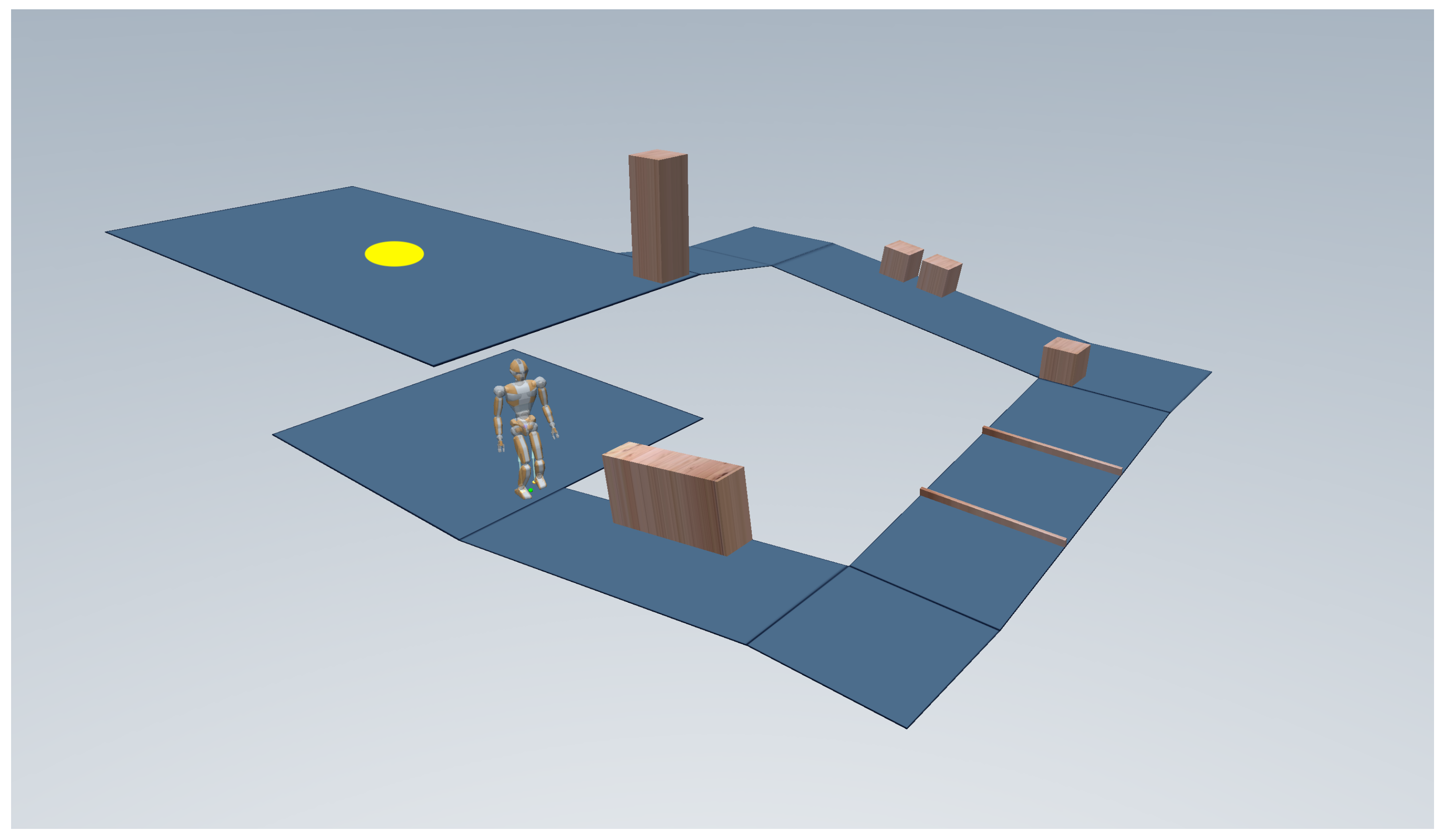
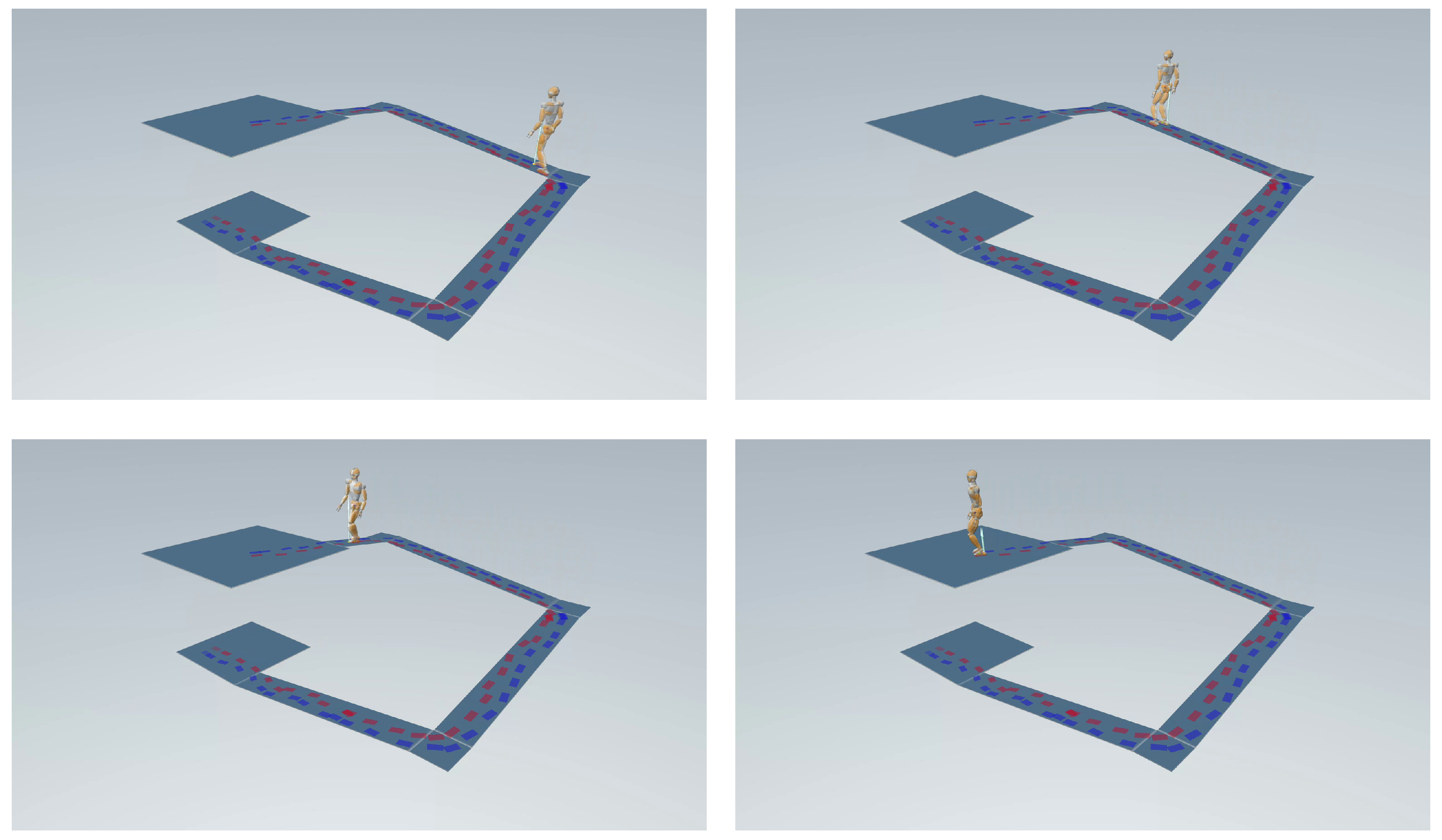
In the situation of interest (Figure 1), a humanoid robot moves in a world of ramps, a specific 3D environment consisting of planar regions that are arbitrarily placed and oriented in space. This characterization encompasses office-like scenarios, with rooms connected by staircases or ramps, possibly arranged on several floors and populated by obstacles. Depending on its elevation and/or inclination, a planar region may be accessible for the humanoid to step on or not.

The mission of the robot is to reach a certain goal area $\mathcal{G}$, assumed to be contained in a single planar region. The locomotion task is accomplished as soon as the robot places a foot inside $\mathcal{G}$.

We wanted to devise a complete framework enabling the humanoid to plan and execute a motion to fulfill the assigned task in the world of ramps. This required addressing two fundamental problems: finding a 3D footstep plan and generating a variable-height gait consistent with such a plan. Footstep planning consists of finding both footstep placements and swing foot trajectories; overall, the footstep plan needed to be feasible (in a sense to be formally defined later) for the humanoid, given the characteristics of the environment. Gait generation consists of finding a CoM trajectory that realizes the footstep plan while guaranteeing the dynamic balance of the robot at all time instants. Starting from the trajectories of the CoM and the feet, a whole-body controller generates torque commands for the robot joints that comply with the robot kinematic and dynamic limitations.

The problem was solved under the following assumptions.

A1

Information about the environment geometry was completely known a priori and collected in a map $\mathcal{M}$ expressed as

$$\mathcal{M}=\{{\mathcal{R}}_1,\dots ,{\mathcal{R}}_n\},$$

(1)

where ${\mathcal{R}}_i$ is an arbitrarily oriented planar region in the 3D space (a ramp).

A2

The humanoid was endowed with a localization module which, using the available sensor data, provided an estimate of the robot’s current state in terms of its CoM and swing foot pose.

In view of assumption A1, a complete footstep plan leading to the goal area $\mathcal{G}$ could be computed offline before the humanoid started to execute the motion. While we maintained this viewpoint in the present study, an extension to the online case could be devised along the same lines of [15], i.e., by updating the footstep plan on the basis of new information gathered and added to $\mathcal{M}$ during the motion, e.g., using visual information [5,6,15].

3. Proposed Approach

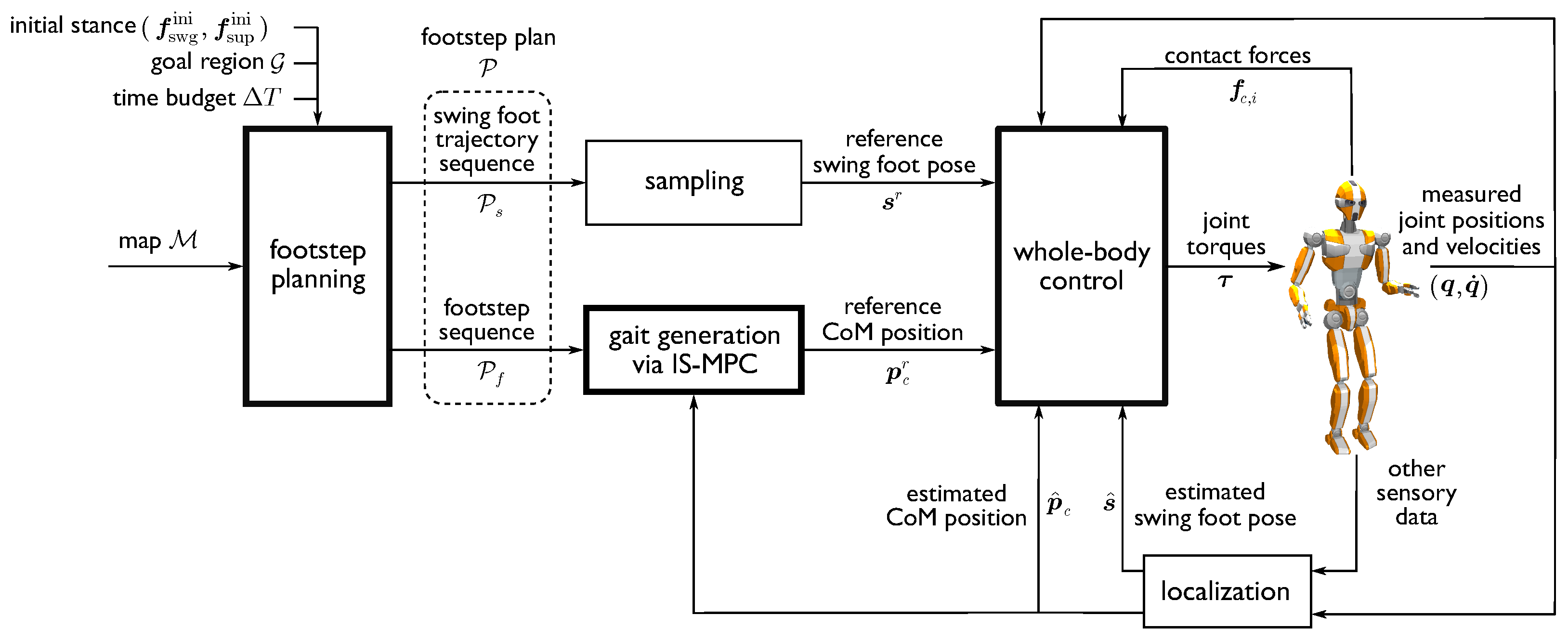
To solve the described problem, we adopted the architecture shown in Figure 2, in which the main components were the footstep planning, gait generation, and whole-body control modules.

In the following, we denote by $\mathit{f}=(x_f,y_f,z_f,{\alpha }_f,{\beta }_f,{\gamma }_f)$ the pose of a footstep, with $x_f$, $y_f$, and $z_f$ representing the coordinates of a representative point, henceforth collectively denoted as ${\mathit{p}}_f$.  ${\alpha }_f,{\beta }_f,{\gamma }_f$ is its orientation, expressed via roll–pitch–yaw angles, collectively denoted as ${\mathit{\varphi }}_f$. Moreover, a pair $({\mathit{f}}_{\mathrm{swg}},{\mathit{f}}_{\sup })$ defines a stance, i.e., the feet poses during a double support phase, after which a step is performed by moving the swing foot from ${\mathit{f}}_{\mathrm{swg}}$ while keeping the support foot at ${\mathit{f}}_{\sup }$.

The footstep planner receives as input the initial humanoid stance $({\mathit{f}}_{\mathrm{swg}}^{\mathrm{ini}},{\mathit{f}}_{\sup }^{\mathrm{ini}})$, the goal area $\mathcal{G}$, a time budget $\Delta T$, and the map $\mathcal{M}$ of the environment.

The time budget is the time afforded to the planner for finding a solution. After each iteration, if the elapsed time exceeds this budget, the algorithm is terminated. At this point, the planner either returns a solution or ends with a failure. Including explicitly this parameter as one of the inputs to the algorithm allowed us to compare different budgets to evaluate the performance of the planning module, but it also paved the way for the extension to the online case as, here, the time budget could be set to be equal to the duration of a step to meet the real-time requirement.

The planner works off-line to find, within $\Delta T$, an optimal footstep plan $\mathcal{P}=\{{\mathcal{P}}_f,{\mathcal{P}}_s\}$ leading to the desired goal area $\mathcal{G}$. In $\mathcal{P}$, we denote by

$${\mathcal{P}}_f=\{{\mathit{f}}^1,\dots ,{\mathit{f}}^n\}$$

(2)

the sequence of footstep placements, whose generic element ${\mathit{f}}^j$ is the pose of the j-th footstep, with ${\mathit{f}}^1={\mathit{f}}_{\mathrm{swg}}^{\mathrm{ini}}$ and ${\mathit{f}}^2={\mathit{f}}_{\sup }^{\mathrm{ini}}$. Also, we denote by

$${\mathcal{P}}_s=\{{\mathit{s}}^1,\dots ,{\mathit{s}}^{n-2}\}$$

(3)

the sequence of associated swing foot trajectories, whose generic element ${\mathit{s}}^j$ is the j-th step, i.e., the trajectory leading the foot from ${\mathit{f}}^j$ to ${\mathit{f}}^{j+2}$ over a fixed duration $T_s$.

Once the footstep plan has been generated, the sequence of footsteps ${\mathcal{P}}_f$ is sent to a gait generation module based on a 3D extension of our Intrinsically Stable MPC (IS-MPC). This module computes in real time a variable-height CoM trajectory that is compatible with ${\mathcal{P}}_f$ and guaranteed to be stable, i.e., bounded with respect to a specific point called the Zero Moment Point (ZMP, more on this in Section 5.1). In particular, we denote by ${\mathit{p}}_c^r$ the current reference position of the CoM produced by IS-MPC. Also, let ${\mathit{s}}^r$ be the current reference pose of the swing foot, obtained by sampling the appropriate subtrajectory in ${\mathcal{P}}_s$.

Finally, the reference trajectories ${\mathit{p}}_c^r$ and ${\mathit{s}}^r$ are passed to a WBC, which computes the joint torque commands $\tau$ for the robot to track these trajectories while ensuring that the generated contact forces are feasible.

Sensor information, including joint encoder data, is used by the localization module to continuously update the estimate of the CoM position and swing foot pose (${\widehat{\mathit{p}}}_c$ and $\widehat{\mathit{s}}$, respectively) through kinematic computations. Finally, these estimates are used to provide feedback to both the gait generation and whole-body control modules.

4. Footstep Planner

The footstep planner takes as input the robot initial stance $({\mathit{f}}_{\mathrm{swg}}^{\mathrm{ini}},{\mathit{f}}_{\sup }^{\mathrm{ini}})$, a goal region $\mathcal{G}$, the time budget $\Delta T$, and the elevation map ${\mathcal{M}}_z$. Based on the given optimality criterion, this module returns the best footstep plan $\mathcal{P}$ to the goal that is found within $\Delta T$.

The planning algorithm builds a tree $\mathcal{T}$, where each vertex $v=({\mathit{f}}_{\mathrm{swg}},{\mathit{f}}_{\sup })$ identifies a stance, and an edge between two vertexes v and $v^{\prime }=({\mathit{f}}_{\mathrm{swg}}^{\prime }={\mathit{f}}_{\sup },{\mathit{f}}_{\sup }^{\prime })$ represents a robot step between the two stances, i.e., a collision-free trajectory such that one foot swings from ${\mathit{f}}_{\mathrm{swg}}$ to ${\mathit{f}}_{\sup }^{\prime }$ and the other remains fixed at ${\mathit{f}}_{\sup }$.

A footstep plan $\mathcal{P}$ to a generic vertex v consists of a branch starting at the root of the tree and connecting it to v. The sequences ${\mathcal{P}}_f$ and ${\mathcal{P}}_s$ for this plan are obtained by collecting respectively the support foot poses of all vertexes and the steps corresponding to all edges along $\mathcal{P}$.

4.1. Footstep Feasibility

Footstep ${\mathit{f}}^j=({\mathit{p}}_f^j,{\mathit{\varphi }}_f^j)=(x_f^j,y_f^j,z_f^j,{\alpha }_f^j,{\beta }_f^j,{\gamma }_f^j)\in {\mathcal{P}}_f$ is feasible if it satisfies the following requirements:

R1

${\mathit{f}}^j$ is fully contained in a single horizontal region.

In practice, one typically uses an enlarged footprint to ensure that this requirement will still be satisfied in the presence of small positioning errors.

R2

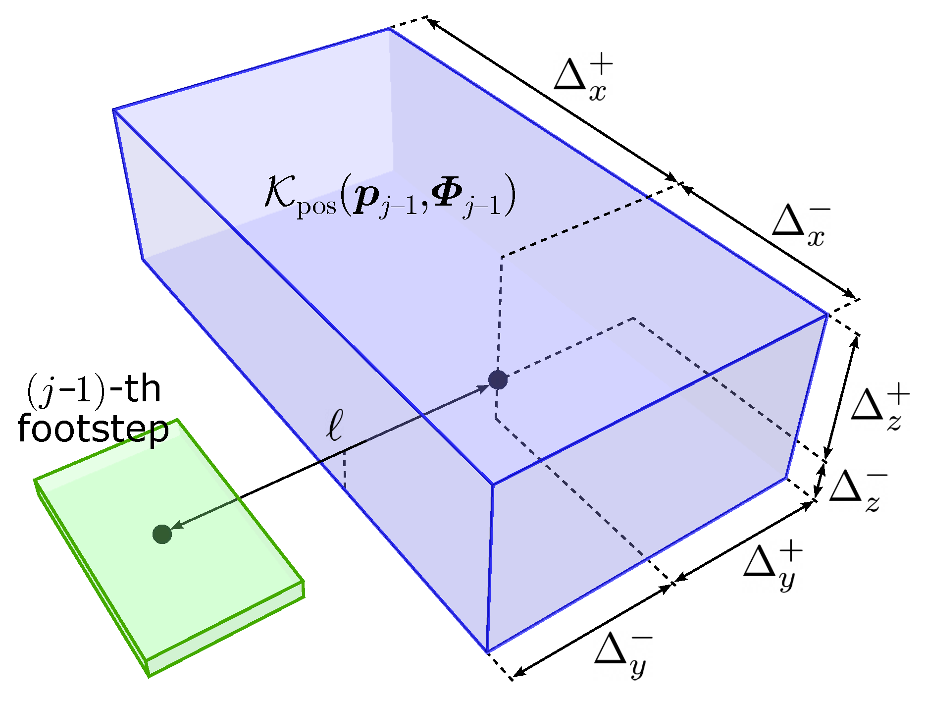
${\mathit{f}}^j$ is kinematically admissible from the previous footstep ${\mathit{f}}^{j-1}$.

Given ${\mathit{f}}^{j-1}$, the kinematically admissible region for ${\mathit{f}}^j$ is the submanifold of ${IR}^3\times SO\left(3\right)$, defined as

$$\mathcal{K}\left({\mathit{f}}_{j-1}\right)={\mathcal{K}}_{\mathrm{pos}}({\mathit{p}}_{j-1},{\mathit{\varphi }}_{j-1})\times {\mathcal{K}}_{\mathrm{ang}}\left({\mathit{\varphi }}_{j-1}\right).$$

(4)

Here, ${\mathcal{K}}_{\mathrm{pos}}({\mathit{p}}_{j-1},{\mathit{\varphi }}_{j-1})$ is the set of kinematically admissible positions of the j-th footstep, defined by the following constraints:

$$-\left(\begin{array}{c}{\Delta }_x^{-}\\ {\Delta }_y^{-}\\ {\Delta }_z^{-}\end{array}\right)\le {\mathit{R}}^T\left({\mathit{\varphi }}_f^{j-1}\right)\left(\begin{array}{c}{x}_f^j-x_f^{j-1}\\ y_f^j-y_f^{j-1}\\ z_f^j-z_f^{j-1}\end{array}\right)\pm \left(\begin{array}{c}0\\ \ell \\ 0\end{array}\right)\le \left(\begin{array}{c}{\Delta }_x^{+}\\ {\Delta }_y^{+}\\ {\Delta }_z^{+}\end{array}\right),$$

(5)

where $\left({\mathit{R}}_f^{j-1}\right)$ is the rotation matrix associated with ${\mathit{\varphi }}_f^{j-1}$ and the $\Delta$ symbols denote lower and upper maximum increments (see Figure 3).

The set ${\mathcal{K}}_{\mathrm{ang}}\left({\mathit{\varphi }}_{j-1}\right)$ of kinematically admissible orientations of the j-th footstep is defined by the following constraints:

$$\begin{array}{c}-{\Delta }_{\alpha }^{-}\le {\alpha }_f^j\le {\Delta }_{\alpha }^{+}\\ -{\Delta }_{\beta }^{-}\le {\beta }_f^j\le {\Delta }_{\beta }^{+}\\ -{\Delta }_{\gamma }^{-}\le {\gamma }_f^j-{\gamma }_f^{j-1}\le {\Delta }_{\gamma }^{+}.\end{array}$$

(6)

Note that the constraints on the roll and pitch angles ${\alpha }_f$ and ${\beta }_f$ are bounds on their value, whereas the constraint on the yaw angle ${\gamma }_f$ only limits its variation with respect to the previous footstep. This is because yaw can assume any value, whereas pitch and roll are subject to kinematic limitations that are impossible to evaluate at the planning stage and must then be accounted for conservatively.

R3

${\mathit{f}}^j$ is reachable from ${\mathit{f}}^{j-2}$ through a collision-free motion.

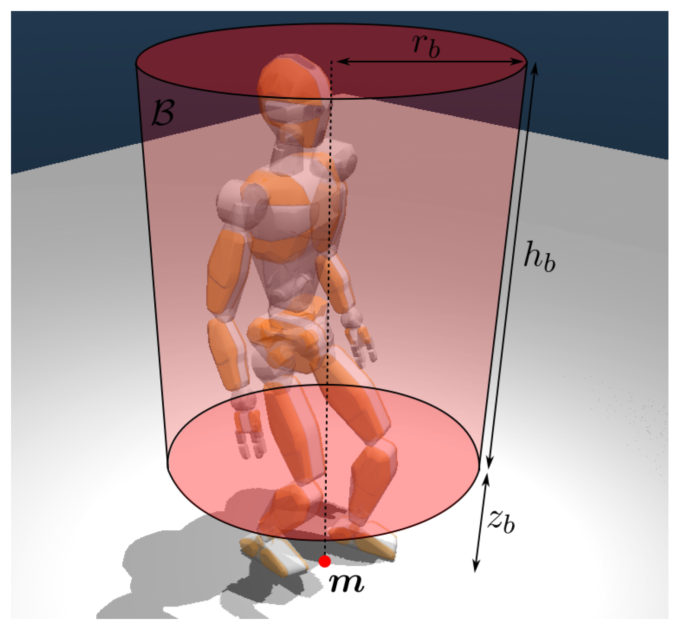
This requirement can only be tested conservatively because information about the whole-body motion of the robot is not yet defined during footstep planning (it will be generated later, in the gait generation phase). In particular, we say that R3 is satisfied if (i) a collision-free swing foot trajectory ${\mathit{s}}^{j-2}$ from ${\mathit{f}}^{j-2}$ to ${\mathit{f}}^j$ exists and (ii) a suitable volume $\mathcal{B}$ accounting for the maximum occupancy of the upper body of the humanoid at stance $({\mathit{f}}^{j-1},{\mathit{f}}^j)$ is collision-free. More precisely, $\mathcal{B}$ is a vertical cylinder whose base has radius $r_b$, centered at the midpoint m between the footsteps, and is raised from the ground by $z_b$, which represents the average distance between the ground and the hip (Figure 4).

4.2. Algorithm

At the start, the tree $\mathcal{T}$ is rooted at $({\mathit{f}}_{\mathrm{swg}}^{\mathrm{ini}},{\mathit{f}}_{\sup }^{\mathrm{ini}})$, i.e., the initial stance of the humanoid. During the exploration, $\mathcal{T}$ is expanded by means of an RRT*-like strategy, whose generic iteration entails the following steps: selecting a vertex for expansion, generating a candidate vertex, choosing a parent for the new vertex and rewiring the tree. We will describe these individual steps below, right after some quick preliminaries.

4.2.1. Preliminaries

We assume that an edge between two vertexes $v^a$ and $v^b$ of $\mathcal{T}$ has a cost $l(v^a,v^b)$. The cost of a vertex v is then defined as

$$c\left(v\right)=c\left(v^{\mathrm{parent}}\right)+l(v^{\mathrm{parent}},v)$$

(7)

and represents the cost of reaching v from the root of $\mathcal{T}$. Then, the cost of a plan $\mathcal{P}$ ending at a vertex v is $c\left(\mathcal{P}\right)=c\left(v\right)$. In this paper, we let $l(v^a,v^b)=1$ for all edges in $\mathcal{T}$. Correspondingly, the cost of a vertex is the length of the corresponding plan in terms of the number of edges (i.e., steps). See [15] for other interesting definitions of the cost of a plan, such as the total height variation or the minimum obstacle clearance.

The algorithm will make use of the set of neighbors of a vertex $v=({\mathit{f}}_{\mathrm{swg}},{\mathit{f}}_{\sup })$, defined as

$$\mathcal{N}\left(v\right)=\{v^{\prime }=({\mathit{f}}_{\mathrm{swg}}^{\prime },{\mathit{f}}_{\sup }^{\prime })\in \mathcal{T}:d_1({\mathit{f}}_{\sup },{\mathit{f}}_{\sup }^{\prime })\le {\overline{d}}_1\},$$

(8)

where

$$d_1(\mathit{f},{\mathit{f}}^{\prime })=\parallel {\mathit{p}}_f-{\mathit{p}}_f^{\prime }\parallel +\sigma |{\mathit{\varphi }}_f-{\mathit{\varphi }}_f^{\prime }|$$

(9)

is the footstep-to-footstep metric, with $\sigma \ge 0$, and  ${\overline{d}}_1$ is a threshold distance.

4.2.2. Selecting a Vertex for Expansion

A point ${\mathit{p}}^{\mathrm{rand}}$ is randomly selected in ${IR}^3$, and the vertex $v^{\mathrm{near}}$ that is closest to ${\mathit{p}}^{\mathrm{rand}}$ is identified according to the following vertex-to-point metric:

$$d_2(v,\mathit{p})={\parallel \mathit{m}\left(v\right)-\mathit{p}\parallel }_{\mathit{W}}+\left|\psi (v,\mathit{p})\right|,$$

(10)

where $\mathit{m}\left(v\right)$ is the midpoint between the feet at stance v, W is a weight matrix, and $\psi (v,\mathit{p})$ is the angle between the ground projection of the robot sagittal axis (whose orientation is the average of the yaw angles of the two footsteps) and the ground projection of the line joining ${\mathit{m}}_{xy}\left(v\right)$ to ${\mathit{p}}_{xy}$. Matrix $\mathit{W}$ can be used to weigh differently vertical and horizontal displacements.

4.2.3. Generating a Candidate Vertex

After identifying the vertex $v^{\mathrm{near}}=({\mathit{f}}_{\mathrm{swg}}^{\mathrm{near}},{\mathit{f}}_{\sup }^{\mathrm{near}})$, a candidate footstep is generated in the kinematically admissible region associated to ${\mathit{f}}_{\sup }^{\mathrm{near}}$. For simplicity, denote by $({\mathit{p}}^{\mathrm{near}},{\mathit{\varphi }}^{\mathrm{near}})$ the pose of ${\mathit{f}}_{\sup }^{\mathrm{near}}$. We first compute the steppable region $\mathcal{S}$ from ${\mathit{f}}_{\sup }^{\mathrm{near}}$, i.e., the intersection between ${\mathcal{K}}_{\mathrm{pos}}({\mathit{p}}^{\mathrm{near}},{\mathit{\varphi }}^{\mathrm{near}})$ and the collection $\mathcal{M}$ of planar regions that constitute the world:

$$\mathcal{S}=\{{\mathcal{K}}_{\mathrm{pos}}({\mathit{p}}^{\mathrm{near}},{\mathit{\varphi }}^{\mathrm{near}})\cap \mathcal{M}\}.$$

(11)

By construction, $\mathcal{S}$ itself will be a collection of planar regions. One of these regions is randomly selected, and a sample point $p^{\mathrm{cand}}$ is extracted from it. Also, a random yaw angle ${\gamma }^{\mathrm{cand}}$ is generated in $[{\gamma }^{\mathrm{near}}-{\Delta }_{\gamma }^{-},{\gamma }^{\mathrm{near}}+{\Delta }_{\gamma }^{+}]$. Finally, we perform foot snapping, a process that correctly places the footstep at $p^{\mathrm{cand}}$, with yaw angle ${\gamma }^{\mathrm{cand}}$, by matching its pitch and roll angles to those of the associated planar region of $\mathcal{S}$.

Once the candidate footstep ${\mathit{f}}^{\mathrm{cand}}$ has been generated, it can be checked with respect to requirement R1 and R2. For the latter, note that the position constraint (5) and the last of the angular constraints (6) are automatically satisfied by the above procedure and, therefore, only the pitch and roll rows of (6) must be explicitly checked.

In order to check requirement R3, we invoke an engine that generates a swing foot trajectory ${\mathit{s}}^{\mathrm{near}}$ from ${\mathit{f}}_{\mathrm{swg}}^{\mathrm{near}}$ to ${\mathit{f}}_{\sup }^{\mathrm{cand}}$. Such an engine uses a Bezier curve as a parameterized trajectory; given the endpoints, such a trajectory can be deformed through control points to change the apex height h along the motion. Once a a swing foot trajectory has been generated, it is checked for collision with the environment: if a collision is detected, h is increased and the process is repeated. If a maximum height $h_{max}$ is reached without success, the candidate footstep is discarded.

If R1–R3 are satisfied, the candidate vertex is generated as $v^{\mathrm{cand}}=({\mathit{f}}_{\mathrm{swg}}^{\mathrm{cand}},{\mathit{f}}_{\sup }^{\mathrm{cand}})$, with ${\mathit{f}}_{\mathrm{swg}}^{\mathrm{cand}}={\mathit{f}}_{\sup }^{\mathrm{near}}$; however, adding $v^{\mathrm{cand}}$ to $\mathcal{T}$ is postponed, as the planner first has to choose a parent for it. If, instead, one of the requirements is violated, we abort the current expansion and start a new iteration.

4.2.4. Choosing a Parent

Although the procedure for generating $v^{\mathrm{cand}}$ originated at $v^{\mathrm{near}}$, a different vertex in the tree might lead to $v^{\mathrm{cand}}$ with a lower cost. To identify such a vertex, the algorithm examines each vertex $v^{\prime }=({\mathit{f}}_{\mathrm{swg}}^{\prime },{\mathit{f}}_{\sup }^{\prime })\in \mathcal{N}\left(v^{\mathrm{cand}}\right)$ to determine whether choosing $v^{\prime }$ as a parent of $v^{\mathrm{cand}}$ satisfies requirements R2-R3 and whether this new connection decreases the cost of $v^{\mathrm{cand}}$, that is

$$c\left(v^{\prime }\right)+l(v^{\prime },v^{\mathrm{cand}})<c\left(v^{\mathrm{near}}\right)+l(v^{\mathrm{near}},v^{\mathrm{cand}}).$$

(12)

The new parent of $v^{\mathrm{cand}}$ is chosen as the vertex $v^{\min }=({\mathit{f}}_{\mathrm{swg}}^{\min },{\mathit{f}}_{\sup }^{\min })$, which allows $v^{\mathrm{cand}}$ to be reached with minimum cost. If $v^{\min }\ne v^{\mathrm{near}}$, the candidate vertex $v^{\mathrm{cand}}$ must be modified by relocating its swing footstep to the support footstep of $v^{\min }$: in particular, a new vertex $v^{\mathrm{new}}=({\mathit{f}}_{\mathrm{swg}}^{\mathrm{new}},{\mathit{f}}_{\sup }^{\mathrm{new}})$ with ${\mathit{f}}_{\mathrm{swg}}^{\mathrm{new}}={\mathit{f}}_{\sup }^{\min }$ and ${\mathit{f}}_{\sup }^{\mathrm{new}}={\mathit{f}}_{\sup }^{\mathrm{cand}}$ is generated and added to $\mathcal{T}$ as a child of $v^{\min }$. The edge joining $v^{\min }$ to $v^{\mathrm{new}}$ represents the swing foot trajectory ${\mathit{s}}^{\min }$.

4.2.5. Rewiring

The last step of each iteration is rewiring, i.e., verifying whether the new node $v^{\mathrm{new}}$ allows some parts of $\mathcal{T}$ to be reached with a lower cost and modifying the tree in accordance. In particular, for each $v^{\prime }=({\mathit{f}}_{\mathrm{swg}}^{\prime },{\mathit{f}}_{\sup }^{\prime })\in \mathcal{N}\left(v^{\mathrm{new}}\right)$, the algorithm checks whether choosing $v^{\mathrm{new}}$ as the parent of $v^{\prime }$ satisfies requirements R2-R3 and whether this connection results in a cost reduction for $v^{\prime }$, that is

$$c\left(v^{\mathrm{new}}\right)+l(v^{\mathrm{new}},v^{\prime })<c\left(v^{\prime }\right).$$

(13)

In this case, $v^{\prime }$ is modified (similarly to what was done in Section 4.2.4) by relocating its swing footstep to ${\mathit{f}}_{\sup }^{\mathrm{new}}$ and then reconnected to $\mathcal{T}$ as a child of $v_{\mathrm{new}}$, with the corresponding edge representing the new swing foot trajectory. Finally, for each child $v^{″}=({\mathit{f}}_{\mathrm{swg}}^{″},{\mathit{f}}_{\sup }^{″})$ of $v^{\prime }$, the swing foot trajectory from the relocated ${\mathit{f}}_{\mathrm{swg}}^{\prime }$ to ${\mathit{f}}_{\sup }^{″}$ is generated and the edge between $v^{\prime }$ and $v^{″}$ is updated.

4.3. Pseudocode

For convenience, the pseudocode of the footstep planning algorithm so far described is given in Algorithm 1.

Algorithm 1 FootstepPlanner()

Require: ${\mathit{f}}_{\mathrm{swg}}^{\mathrm{ini}}$, ${\mathit{f}}_{\sup }^{\mathrm{ini}}$, $\Delta T$, $\mathcal{M}$  Initialize($\mathcal{T},({\mathit{f}}_{\mathrm{swg}}^{\mathrm{ini}}$, ${\mathit{f}}_{\sup }^{\mathrm{ini}}$))  while TimeNotExpired($\Delta T$) do     ${\mathit{p}}^{\mathrm{rand}}$← RandomPointGenerator$\left(\right)$     $v^{\mathrm{near}}$← NearestNeighborVertex($\mathcal{T}$, ${\mathit{p}}^{\mathrm{rand}}$)     ${\mathit{f}}^{\mathrm{cand}}$← GenerateCandidateFootstep(${\mathit{f}}_{\sup }^{\mathrm{near}},\mathcal{M}$)     if R1(${\mathit{f}}^{\mathrm{cand}}$) AND R2(${\mathit{f}}^{\mathrm{cand}}$) then       ${\mathit{s}}^{\mathrm{near}}$← SwingTrajectoryGenerator(${\mathit{f}}_{\mathrm{swg}}^{\mathrm{near}},{\mathit{f}}_{\sup }^{\mathrm{cand}}$)       if R3(${\mathit{s}}^{\mathrm{near}}$) then          $v^{\mathrm{cand}}\leftarrow ({\mathit{f}}_{\sup }^{\mathrm{near}},{\mathit{f}}_{\sup }^{\mathrm{cand}})$          $\mathcal{N}\leftarrow$ Neighbors($\mathcal{T},v^{\mathrm{cand}}$)          $(v^{\min },{\mathit{s}}^{\min })\leftarrow$ ChooseParent($\mathcal{T},\mathcal{N},v^{\mathrm{near}},v^{\mathrm{cand}},{\mathit{s}}^{\mathrm{near}}$)          $v^{\mathrm{new}}\leftarrow ({\mathit{f}}_{\sup }^{\min },{\mathit{f}}_{\sup }^{\mathrm{cand}})$          $\mathcal{T}\leftarrow$ AddVertex($v^{\min },v^{\mathrm{new}},{\mathit{s}}^{\min }$)          Rewire($\mathcal{T},\mathcal{N},v^{\mathrm{new}}$)       end if     end if  end while  return

When the time budget $\Delta T$ expires, we stop tree expansion and retrieve ${\mathcal{V}}_{\mathrm{goal}}$, the set of vertexes v such that ${\mathit{p}}_{f,\sup }\in \mathcal{G}$. From this, we extract the vertex with minimum cost and obtain the optimal footstep plan $\mathcal{P}$ as the branch of $\mathcal{T}$ joining the root to $v^{*}$.

4.4. Footstep Planning: Numerical Results

The proposed footstep planner was implemented in C++ 17 on a laptop equipped with an AMD Ryzen 7 6800HS CPU and an NVIDIA GeForce RTX 3050 GPU. The chosen humanoid was JVRC1, an open-source virtual robot with a total of 44 joints created for the Japan Virtual Robotics Challenge [17]. JVRC1 is similar to the HRP series of humanoids in terms of mechanical design, thus representing a realistic yet convenient simulation platform.

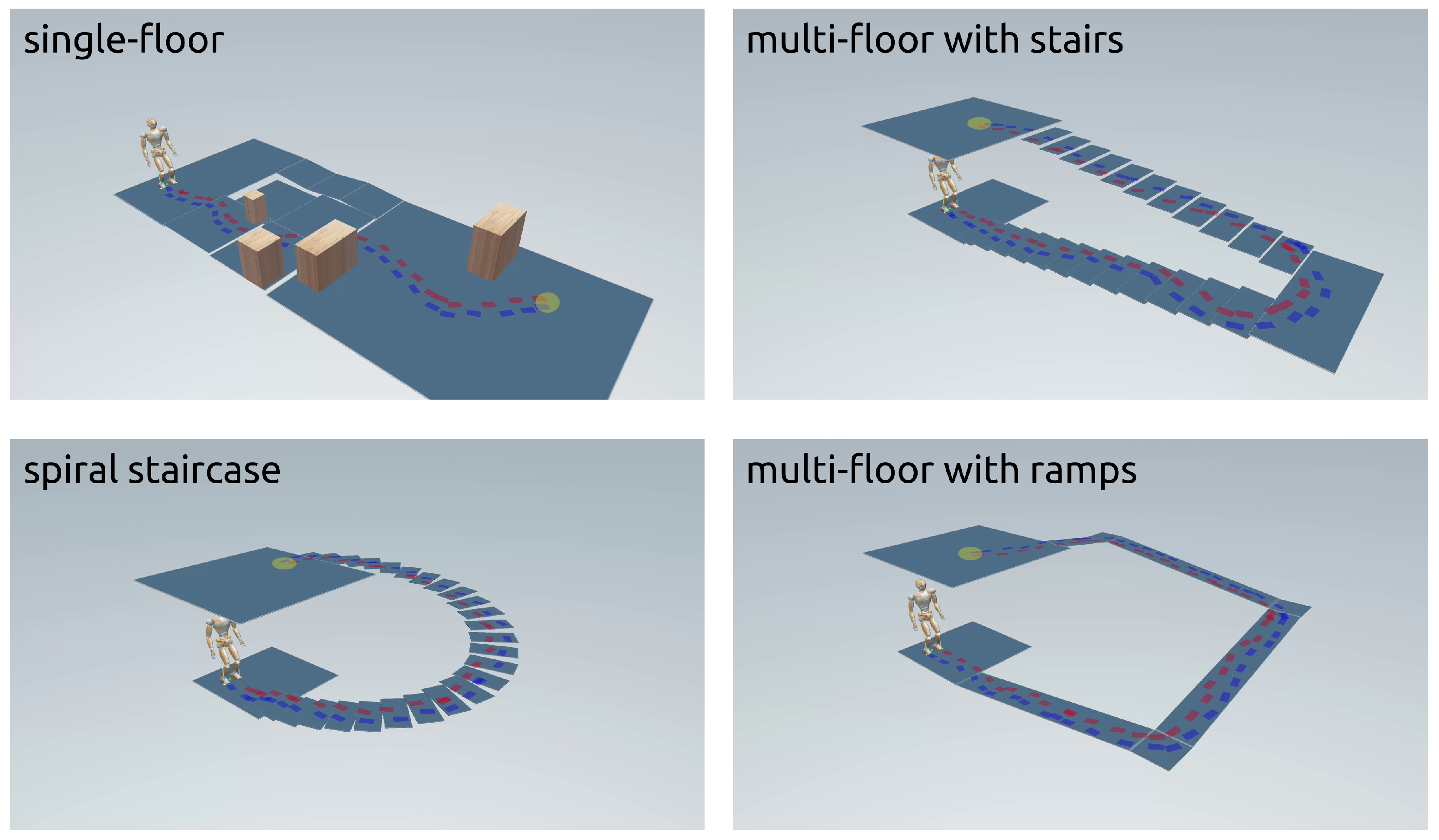
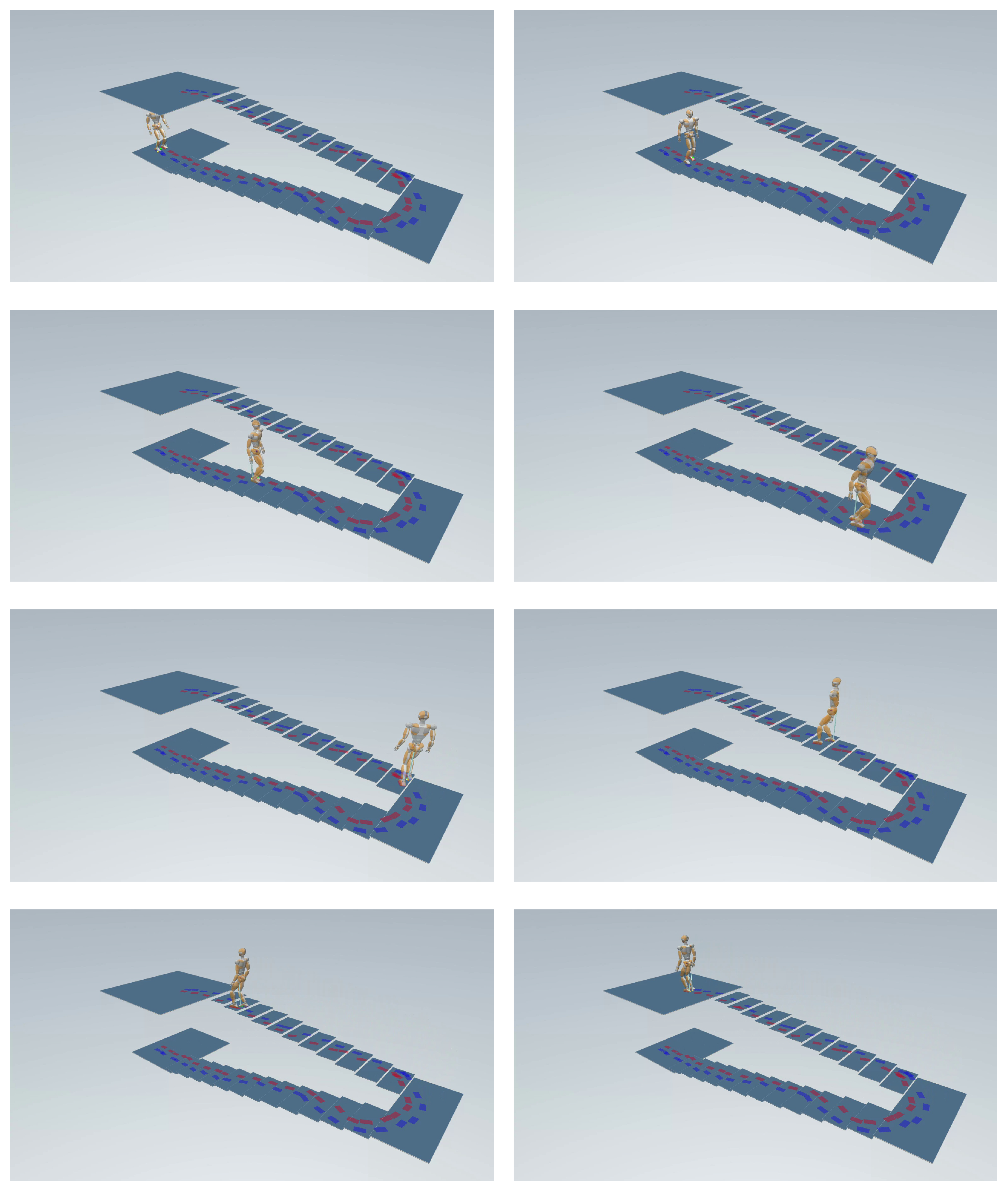
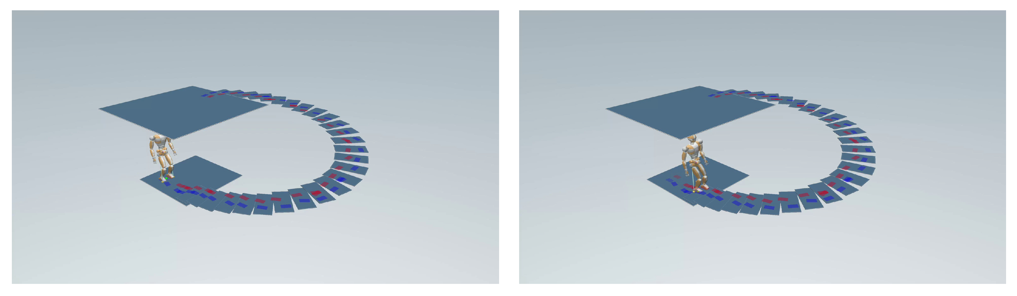
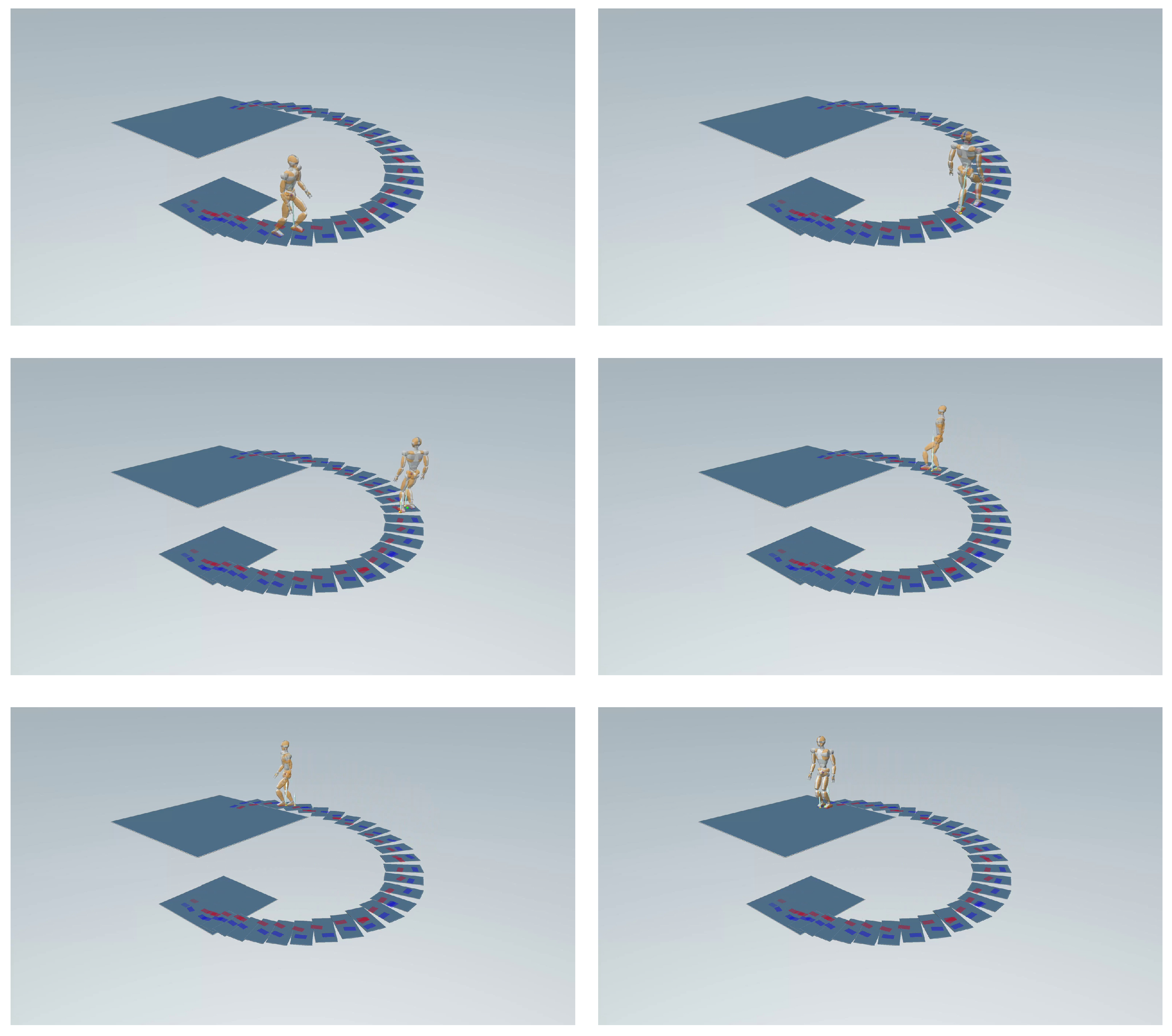
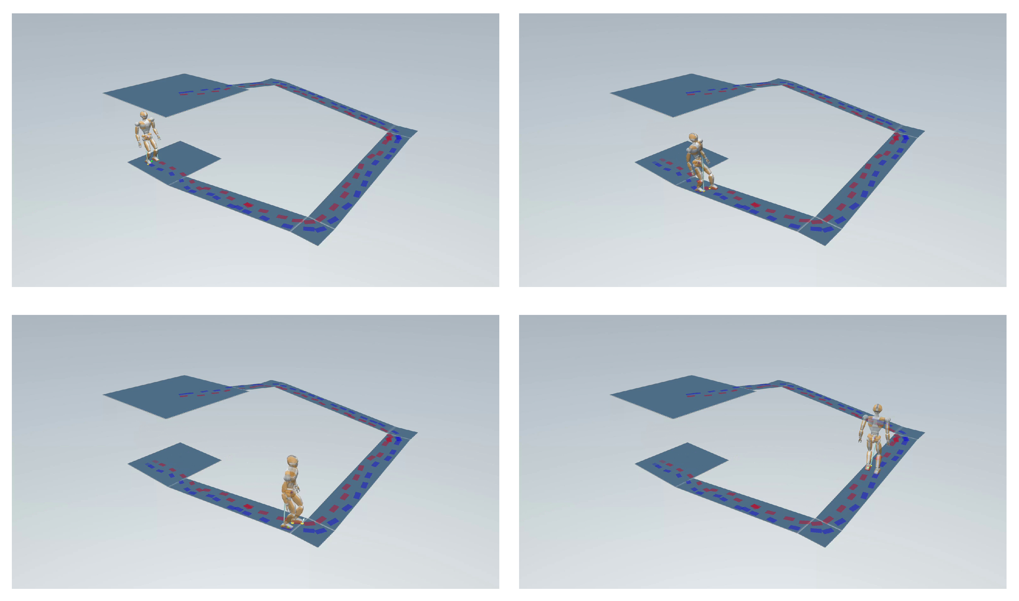
A campaign of planning experiments took place over four scenarios of varying complexity (see Figure 5):

• Single Floor. This environment included elevation changes, ramps (both ascending and descending), and obstacles.
• Multi-Floor with Stairs. This was an environment with two floors connected by 23 steps.
• Spiral Staircase. A spiral staircase with 26 steps connected two floors.
• Multi-Floor with Ramps. In this environment, the two floors were connected by four inclined ramps and three landings.

In all scenarios, the robot had to reach a circular goal region with a radius of 0.3 m. In the footstep planner, we set $h_{max}=0.19$ m, ${\Delta }_x^{-}=0.05$ m, ${\Delta }_x^{+}=0.30$ m, ${\Delta }_y^{-}=0.20$ m, ${\Delta }_y^{+}=0.30$ m, ${\Delta }_z^{-}={\Delta }_z^{+}=0.12$ m, ${\Delta }_{\alpha }^{-}={\Delta }_{\alpha }^{+}=0.175$ rad, ${\Delta }_{\beta }^{-}={\Delta }_{\beta }^{+}=0.175$ rad, ${\Delta }_{\gamma }^{-}={\Delta }_{\gamma }^{+}=0.35$ rad, $z_b=0.3$ m, $h_b=1.2$ m, and $r_b=0.25$ m.

Figure 5 shows some examples of successful footstep plans obtained in the four scenarios using the proposed algorithm.

Table 1. Performance of the footstep planner in the four scenarios.

Scenario	Time Budget [s]	Avg Cost	Min Cost	Max Cost	Iters	Tree Size	1st Plan [s]	Successes
Single-Floor	10	57.3	46.0	67.0	10,685	7392	4.0	19/30
	30	61.5	49.0	83.0	18,458	12,890	11.22	28/30
	60	61.3	46.0	75.0	26,370	18,457	13.67	29/30
Multi-Floor with Stairs	10	94.0	86.0	104.0	11,290	7026	6.27	14/30
	30	94.2	85.0	102.0	19,297	12,500	8.94	27/30
	60	93.3	78.0	103.0	27,933	18,119	12.51	29/30
Spiral Staircase	10	73.3	68.0	114.0	13,316	6654	3.98	24/30
	30	72.8	59.0	108.0	21,771	12,291	5.37	29/30
	60	66.9	59.0	73.0	29,247	17,571	5.59	30/30
Multi-Floor with Ramps	10	103.7	100.0	111.0	10,382	7997	8.64	3/30
	30	110.0	96.0	123.0	17,765	13,876	19.73	19/30
	60	107.5	94.0	130.0	25,924	19,695	21.88	29/30

gives details about the performance of the planner in each scenario, for different values of the time budget, with each row reporting average results over 30 runs of the planner (the first plan was the time needed by the footstep planner to generate the first plan that reached the goal). A run was considered unsuccessful if the planner terminated without placing any footstep in the goal region. Note that increasing the time budget consistently improved the success rate, suggesting that the proposed footstep planner is probabilistically complete.

Overall, the results highlight the effectiveness of the proposed planner in rather complex 3D scenarios, even in the presence of stairs and ramps. See the concluding section for some hints at possible improvements of our planner.

5. Control Architecture

This section describes the control pipeline, which consisted of the IS-MPC module followed by the WBC module (see Figure 2).

5.1. IS-MPC Gait Generation

Gait generation was the process of generating a feasible trajectory for the CoM position ${\mathit{p}}_c=(x_c,y_c,z_c)$, such that the robot realized the assigned footstep plan and maintained balance. This last requirement could be formulated as a constraint on the position ${\mathit{p}}_z=(x_z,y_z,z_z)$ of the Zero Moment Point (ZMP), which was the point of application of the equivalent ground reaction force.

To generate the CoM trajectory, we used MPC, which optimized trajectories over a certain horizon, using a model to predict the evolution of the system.

5.1.1. Prediction Model

Our prediction model is a 3D extension of the classic LIP, which has the ZMP as input and allows for vertical motion of the CoM [14]. By neglecting the internal angular momentum variation, we have

$$\begin{array}{ccc}\hfill (z_c-z_z){\ddot{x}}_c& =& (x_c-x_z)({\ddot{z}}_c+g)\hfill \\ \hfill (z_c-z_z){\ddot{y}}_c& =& (y_c-y_z)({\ddot{z}}_c+g),\hfill \end{array}$$

where g is the gravity acceleration. To remove the nonlinear coupling between the horizontal and vertical components, we impose $({\ddot{z}}_c+g)/(z_c-z_z)={\eta }^2$, where $\eta$ is a constant parameter. The resulting model is expressed as

$${\ddot{\mathit{p}}}_c={\eta }^2({\mathit{p}}_c-{\mathit{p}}_z)+\mathit{g},$$

(14)

where $\mathit{g}=(0,0,-g)$ is a constant drift. This means that the 3D LIP is at an equilibrium when the CoM and ZMP are vertically displaced by $\eta /g$; this should be taken into account when choosing the value of $\eta$. In our formulation, we dynamically extended (14) so that the input was the ZMP velocity ${\dot{\mathit{p}}}_z$, rather than the position ${\mathit{p}}_z$, in order to generate smoother trajectories.

5.1.2. ZMP Constraints

In the classic LIP, the condition for balance requires the ZMP to stay within of the support polygon of the robot, which, however, is no more defined in a 3D setting. A sufficient condition for ensuring balance in this case is that the ZMP must belong to a pyramidal region $\mathcal{Z}$, with apex at the robot CoM and edges going through the vertexes of the convex hull of the contact surfaces. Since this condition is nonlinear, we resorted to the following conservative approximation.

Consider a moving box $\mathcal{B}$ with constant dimensions $(d_x,d_y,d_z)$ along the three axes. Its center ${\mathit{p}}_{\mathrm{mc}}=(x_{\mathrm{mc}},y_{\mathrm{mc}},z_{\mathrm{mc}})$ moves in the following way: during single support phases, it coincides with the position of the support foot, while, during double support phases, it performs a roto-translation from the position of the previous support foot to the position of the next. By properly choosing $d_x$, $d_y$, and $d_z$, one may guarantee that $\mathcal{B}$ is always contained in $\mathcal{Z}$ [15].

At a generic time instant $t_j$, a linear ZMP constraint can then be written as

$$-{\displaystyle \frac{1}{2}}\left(\begin{array}{c}{d}_x\\ d_y\\ d_z\end{array}\right)\le {\mathit{R}}_j^T({\mathit{p}}_z^j-{\mathit{p}}_{\mathrm{mc}}^j)\le {\displaystyle \frac{1}{2}}\left(\begin{array}{c}{d}_x\\ d_y\\ d_z\end{array}\right),$$

(15)

where ${\mathit{R}}_j$ is the rotation matrix associated with the orientation of the moving box at $t_j$ and the j superscript denotes the variable at $t_j$.

5.1.3. Stability Constraint

While keeping the ZMP inside $\mathcal{B}$ (and therefore, inside $\mathcal{Z}$) is sufficient for balance, it does not by itself guarantee that the COM trajectories are bounded with respect to the ZMP. This is due to the well-known fact that the LIP model includes one unstable mode, which can be isolated by defining the variable ${\mathit{p}}_u={\mathit{p}}_c+{\dot{\mathit{p}}}_c/\eta$.

To avoid divergence, IS-MPC enforces the following stability condition:

$${\mathit{p}}_u^k=\eta {\int }_{t_k}^{\infty }{e}^{-\eta (\tau -t_k)}{\mathit{p}}_z\left(\tau \right)d\tau +{\displaystyle \frac{\mathit{g}}{\eta }}.$$

(16)

This is a relationship between the current value of ${\mathit{p}}_u$ and the future of the ZMP trajectory and is, therefore, noncausal. To obtain a causal condition, we split the integral in two parts, the first from $t_k$ to $t_{k+C}$ (the final instant of the prediction horizon) and the second from $t_{k+C}$ to infinity. While the first integral could be expressed in terms of the MPC decision variables ${\dot{\mathit{p}}}_z^k,\dots ,{\dot{\mathit{p}}}_z^{k+C-1}$, the second could be computed by conjecturing a trajectory ${\tilde{\mathit{p}}}_z$ of ${\mathit{p}}_z$ (anticipative tail) on the basis of information contained in the footstep plan:

$${\mathit{c}}_u^k=\eta {\int }_{t_{k+C}}^{\infty }{e}^{-\eta (\tau -t_k)}{\tilde{\mathit{p}}}_z\left(\tau \right)d\tau .$$

(17)

The stability constraint could then be written as

$${\mathit{p}}_u^k=\eta {\int }_{t_k}^{t_{k+C}}{e}^{-\eta (\tau -t_k)}{\mathit{p}}_z\left(\tau \right)d\tau +{\mathit{c}}_u^k+{\displaystyle \frac{\mathit{g}}{\eta }}.$$

(18)

5.1.4. IS-MPC

At each iteration, IS-MPC solved the following quadratic program:

$$\begin{array}{cc}\hfill \underset{{\dot{\mathit{p}}}_z^k,\dots ,{\dot{\mathit{p}}}_z^{k+C-1}}{min}& \sum _{i=k}^{k+C-1}\left|\right|{\dot{\mathit{p}}}_z^i{\left|\right|}^2+\lambda \left|\right|{\mathit{p}}_z^i-{\mathit{p}}_{\mathrm{mc}}^i{\left|\right|}^2\hfill \\ \hfill \mathrm{subject} \mathrm{to}:& \mathrm{ZMP} \mathrm{constraints} \left(15\right), \mathrm{for}j=k,\dots ,k+C\hfill \\ \hfill & \mathrm{stability} \mathrm{constraint} \left(18\right),\hfill \end{array}$$

(19)

where $\lambda$ is a positive weight. After solving the quadratic program, the first optimal sample ${\dot{\mathit{p}}}_z^k$ was used to integrate the dynamically extended model (14) and obtain the next sample of the reference CoM position ${\mathit{p}}_c^{\ast }$ and velocity ${\dot{\mathit{p}}}_c^{\ast }$, as well as of the corresponding ZMP position ${\mathit{p}}_z^{\ast }$. The corresponding CoM acceleration could then be computed from (14). All these terms were sent to the WBC, where they were used to set up the CoM tracking task.

5.2. Whole-Body Controller

Commands to be sent to the robot joints were generated by a whole-body controller that worked in two stages. The first stage determined appropriate joint accelerations and contact forces by solving a constrained quadratic program and the second stage computed the associated joint torques via inverse dynamics.

5.2.1. Task References

The input to the WBC is a set of reference trajectories, one for each task. The set of tasks was $\mathcal{T}=$ {com, left, right, torso, joint}, which respectively represented

• com: the CoM reference, generated by the IS-MPC module;
• left/right: foot pose references, generated by the footstep planner;
• torso: a reference torso orientation, typically chosen to be upright;
• joint: a reference joint posture (for solving kinematic redundancy).

We denoted the generic task variable by ${\mathit{t}}_i$, $i=1,\dots ,n_t$, and its reference position, velocity, and acceleration by ${\mathit{t}}_i^{\ast }$, ${\dot{\mathit{t}}}_i^{\ast }$, and ${\ddot{\mathit{t}}}_i^{\ast }$, respectively (with a little abuse as we also used a time derivative notation for angular task variables). The desired acceleration ${\ddot{\mathit{t}}}_i$ was then defined as

$${\ddot{\mathit{t}}}_i={\ddot{\mathit{t}}}_i^{\ast }+k_p({\mathit{t}}_i^{\ast }-{\mathit{t}}_i)+k_d({\dot{\mathit{t}}}_i^{\ast }-{\dot{\mathit{t}}}_i),$$

(20)

where the reference acceleration was used as feedforward and the PD feedback was aimed at robustifying kinematic inversion. The desired acceleration ${\ddot{\mathit{t}}}_i$ was realized provided that the following relationship held:

$${\mathit{J}}_i\dot{\mathit{\nu }}+{\dot{\mathit{J}}}_i\mathit{\nu }={\ddot{\mathit{t}}}_i^{\ast }+k_p({\mathit{t}}_i^{\ast }-{\mathit{t}}_i)+k_d({\dot{\mathit{t}}}_i^{\ast }-{\dot{\mathit{t}}}_i),$$

(21)

where ${\mathit{J}}_i$ is the Jacobian of the i-th task.

5.2.2. Robot Dynamics

The robot dynamics can be written as

$$\mathit{M}\left(\mathit{q}\right)\dot{\mathit{\nu }}+\mathit{n}(\mathit{q},\mathit{\nu })=\left(\begin{array}{c}\mathbf{0}\\ \mathit{\tau }\end{array}\right)+\sum _{i=1}^{n_c}{\mathit{J}}_{c,i}^T\left(\mathit{q}\right){\mathit{f}}_{c,i}.$$

(22)

Here, $\mathit{M}$ is the inertia matrix; the configuration $\mathit{q}=({\mathit{q}}_u,{\mathit{q}}_a)$ is the stack of the floating base (unactuated) variables and the joint (actuated) variables; $\mathit{\nu }=({\mathit{\nu }}_u,{\dot{\mathit{q}}}_a)$ contains the corresponding pseudovelocities; $\mathit{n}$ collects Coriolis, centrifugal, and gravitational terms; $\mathit{\tau }$ are the joint torques; and ${\mathit{J}}_{c,i}$ denotes the Jacobian of the point of application of the i-th contact force ${\mathit{f}}_{c,i}$, with $i=1,\dots ,n_c$.

Equation (22) can be partitioned to highlight the unactuated and the actuated dynamics:

$$\left(\begin{array}{c}{\mathit{M}}_u\\ {\mathit{M}}_a\end{array}\right)\dot{\mathit{\nu }}+\left(\begin{array}{c}{\mathit{n}}_u\\ {\mathit{n}}_a\end{array}\right)=\left(\begin{array}{c}\mathbf{0}\\ \mathit{\tau }\end{array}\right)+\sum _{i=1}^{n_c}\left(\begin{array}{c}{\mathit{J}}_{ci,u}^T\\ {\mathit{J}}_{ci,a}^T\end{array}\right){\mathit{f}}_{c,i},$$

(23)

We omit the dependence on q and v for compactness.

5.2.3. Constraints

The first constraint enforces the unactuated part of (23):

$${\mathit{M}}_u\dot{\mathit{\nu }}+{\mathit{n}}_u=\sum _{i=1}^{n_c}{\mathit{J}}_{ci,u}^T{\mathit{f}}_{c,i}.$$

(24)

We did not directly enforce the actuated dynamics (which would have required adding $\mathit{\tau }$ as a decision variable) because $\mathit{\tau }$ did not explicitly appear in our quadratic program; therefore, it was computed a posteriori from the inverse dynamics without affecting the optimization process (if one wants to minimize torque effort or impose torque limits, $\mathit{\tau }$ must be included in the decision variables, and then the actuated dynamics should be added as a constraint).

The second set of constraints guarantee stationary contacts by imposing zero acceleration to the left and/or right foot, depending on the specific support phase:

$${\mathit{J}}_{\mathrm{left}/\mathrm{right}}\dot{\mathit{\nu }}+{\dot{\mathit{J}}}_{\mathrm{left}/\mathrm{right}}\mathit{\nu }=\mathbf{0}.$$

(25)

The third set of constraints enforce limits on joint velocities and positions:

$${\dot{\mathit{q}}}_{a,min}\le {\dot{\mathit{q}}}_a+\delta {\ddot{\mathit{q}}}_a\le {\dot{\mathit{q}}}_{a,max}$$

(26)

$${\mathit{q}}_{a,min}\le {\mathit{q}}_a+\delta {\dot{\mathit{q}}}_a+\frac{{\delta }^2}{2}{\ddot{\mathit{q}}}_a\le {\mathit{q}}_{a,max},$$

(27)

where $\delta$ is the duration of a sampling interval.

The last set of constraints require each contact force ${\mathit{f}}_{c,i}$ to be contained in the friction cone, ensuring that no slipping occurs:

$$-\mu f_{ci,n}\le f_{ci,x}\le \mu f_{ci,n}$$

(28)

$$-\mu f_{ci,n}\le f_{ci,y}\le \mu f_{ci,n},$$

(29)

where $\mu$ is the friction coefficient, $f_{ci,n}$ is the normal component of ${\mathit{f}}_{c,i}$, and $f_{ci,x},f_{ci,y}$ are its tangential components along the x and y axes of the foot frame at the contact. Note that (i) a pyramidal approximation of the friction cone was used to maintain linearity and (ii) these constraints automatically implied $f_{ci,n}>0$, i.e., unilaterality of the contact forces.

5.2.4. Quadratic Program

At each iteration, the first stage of the WBC solved the following QP problem:

$$\begin{array}{cc}\hfill \underset{\dot{\mathit{\nu }},{\mathit{f}}_1,\dots ,{\mathit{f}}_{n_c}}{min}& \sum _{i=1}^{n_t}{w}_i{∥{\mathit{J}}_i\dot{\mathit{\nu }}+{\dot{\mathit{J}}}_i\mathit{\nu }-{\ddot{\mathit{t}}}_i^{\ast }-k_p({\mathit{t}}_i^{\ast }-{\mathit{t}}_i)-k_d({\dot{\mathit{t}}}_i^{\ast }-{\dot{\mathit{t}}}_i)∥}^2\hfill \\ \hfill \mathrm{subject}\mathrm{to}& \mathrm{unactuated}\mathrm{dynamics}\left(24\right),\hfill \\ \hfill & \mathrm{stationary}\mathrm{contact}\mathrm{constraints}\left(25\right),\hfill \\ \hfill & \mathrm{joint}\mathrm{velocity}\mathrm{constraints}\left(26\right),\hfill \\ \hfill & \mathrm{joint}\mathrm{position}\mathrm{constraints}\left(27\right),\hfill \\ \hfill & \mathrm{contact}\mathrm{force}\mathrm{constraints}\left(28\right),\left(29\right),i=1,\dots ,n_c.\hfill \end{array}$$

(30)

5.2.5. Inverse Dynamics

Once $\dot{\mathit{\nu }}$ and the contact forces ${\mathit{f}}_{c,i}$ were obtained by solving the above QP, the joint torques could be computed using the actuated dynamics in (23), i.e.,

$$\mathit{\tau }={\mathit{M}}_a\dot{\mathit{\nu }}+{\mathit{n}}_a-\sum _{i=1}^{n_c}{\mathit{J}}_{ci,a}^T{\mathit{f}}_{c,i}.$$

(31)

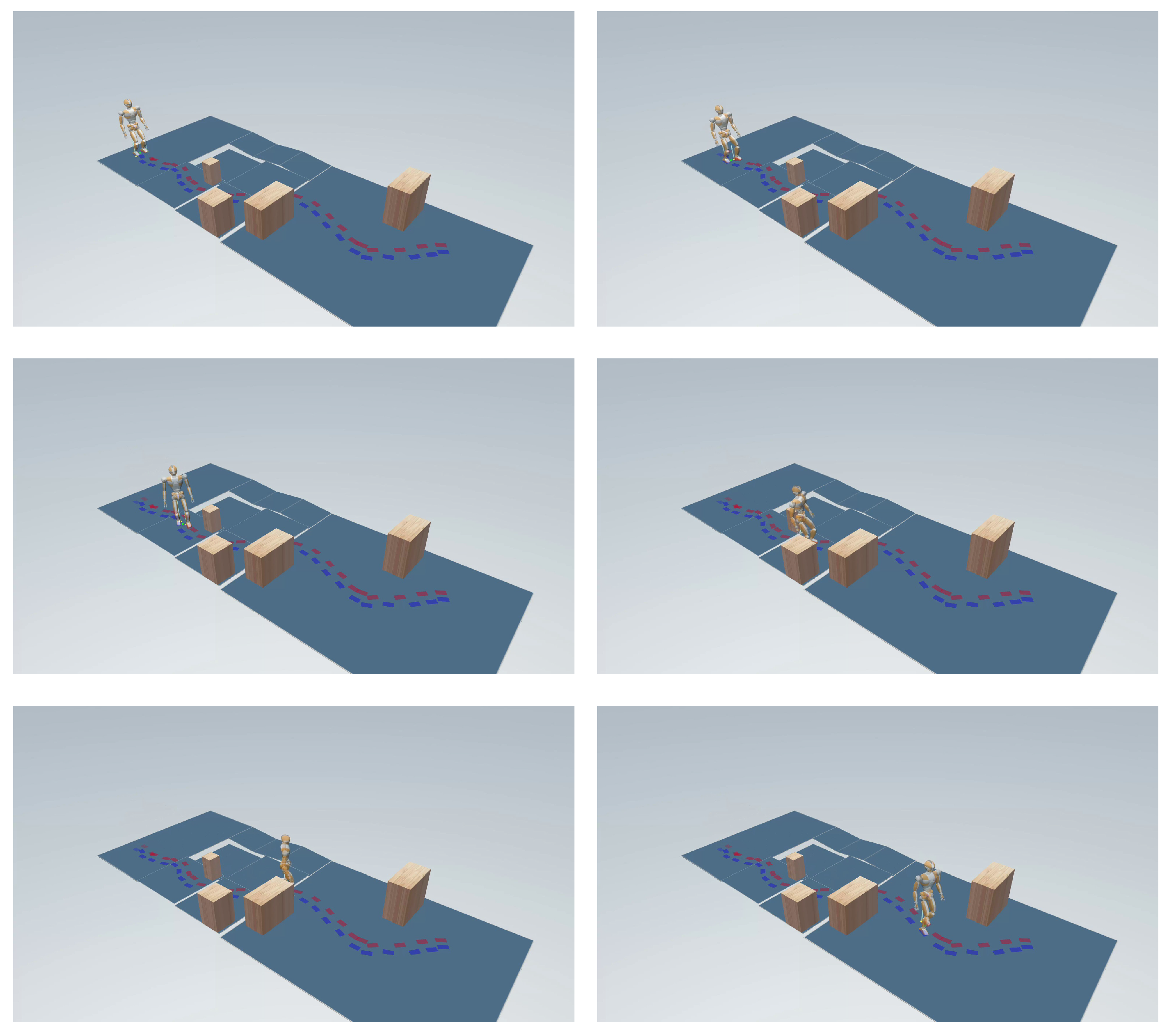
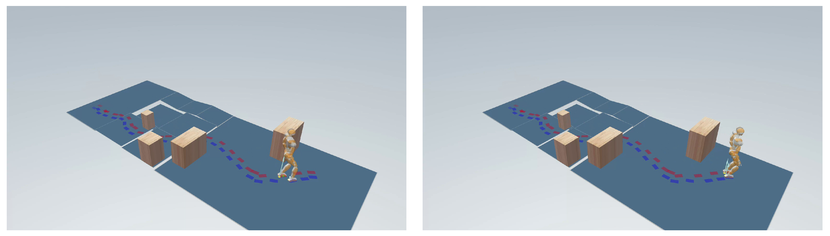
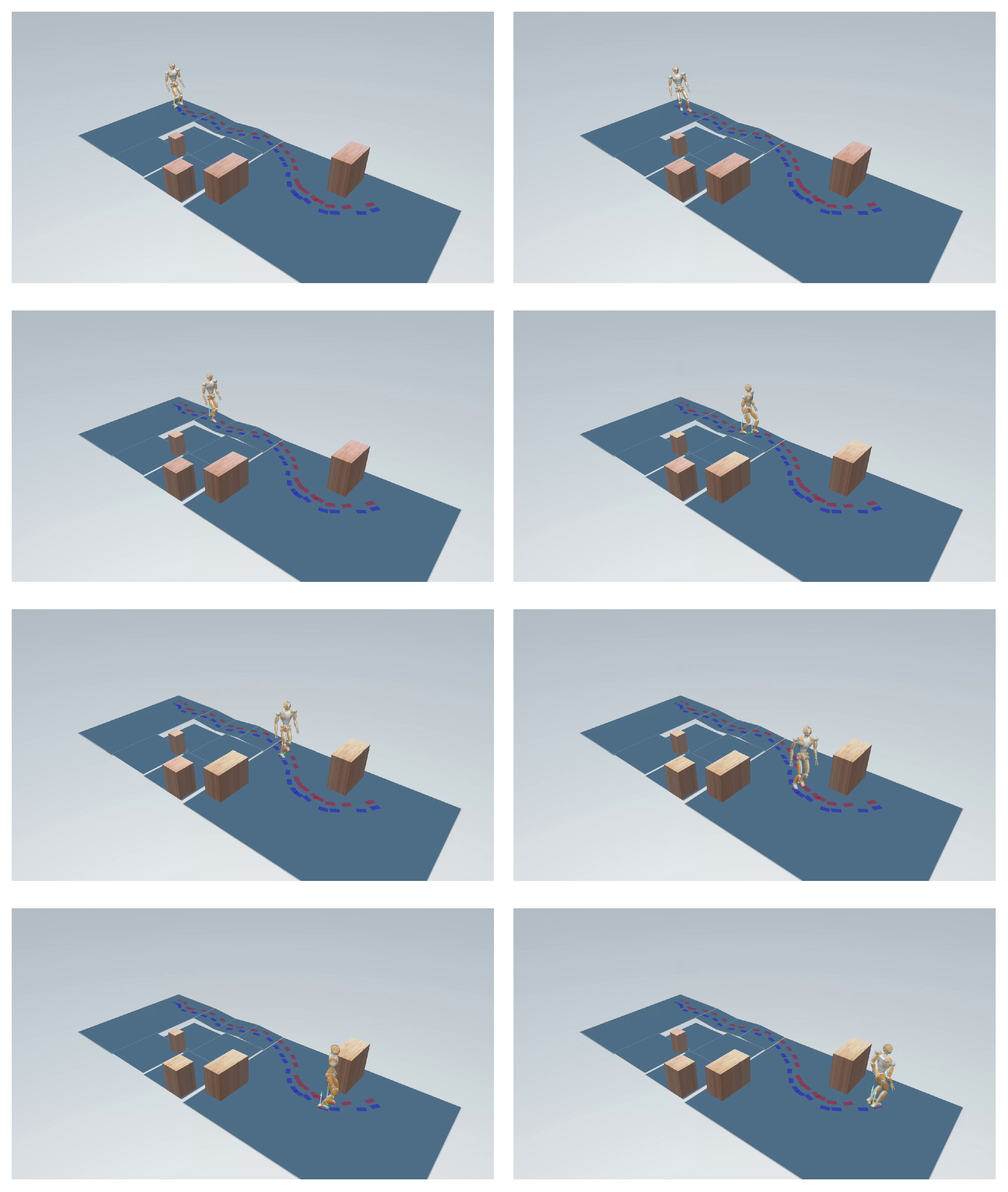
6. Simulations

We now complement the footstep planning results of Section 4.4 by presenting dynamic simulations of the JVRC1 robot executing the planned motions in MuJoCo, which guaranteed high physical accuracy. IS-MPC ran at 100 Hz and used a sampling interval of 0.1 s and a control horizon of 2 s, whereas the WBC ran at 1000 Hz (i.e., $\delta =1$ ms). Contacts were modeled with four forces per foot, so that $n_c=4$ or 8 depending on the support phase. Finally, all quadratic programs (QPs) were solved with HPIPM [18], which required under $1\mathrm{ms}$ to compute a solution, ensuring real-time capability.

The simulation results are shown via successive snapshots in Figure 6, Figure 7, Figure 8, Figure 9 and Figure 10 and in the form of video clips at https://youtu.be/RFPrQjY2tD8 (accessed on 11 June 2025). As expected, the robot was able to efficiently and robustly realize all footstep plans, even in the presence of stairs or inclined ramps.

7. Conclusions

The proposed framework represents a humanoid motion generation scheme that enables navigation in complex 3D environments, including multiple floors and inclined surfaces. We ran an extensive campaign in order to validate the performance of the pipeline (footstep planner, gait generation, and whole body control) in several different scenarios via dynamic simulations on a JVRC1 robot in MuJoCo. Our results show that our framework is effective and robust in very complex environments, paving the way for further promising research.

Future work will explore several directions, including

• implementing and testing the proposed method on the Unitree G1 humanoid available in our lab;
• speeding up the footstep planner by adopting a k-d tree [16] data structure and introducing waypoints (intermediate goals);
• devising an online version of the planner that can be used as the robot moves and gathers new information about the environment;
• using a whole-body MPC for enhancing agility and allowing more complex movements.

References

- Hauser, K.; Bretl, T.; Latombe, J.C.; Harada, K.; Wilcox, B. Motion Planning for Legged Robots on Varied Terrain. Int. J. Robot. Res. 2008, 27, 1325–1349. [Google Scholar] [CrossRef]
- Chestnutt, J.; Lau, M.; Cheung, G.; Kuffner, J.; Hodgins, J.; Kanade, T. Footstep Planning for the Honda ASIMO Humanoid. In Proceedings of the 2005 IEEE International Conference on Robotics and Automation, Barcelona, Spain, 18–22 April 2005; pp. 629–634. [Google Scholar]
- Gutmann, J.S.; Fukuchi, M.; Fujita, M. Real-time path planning for humanoid robot navigation. In Proceedings of the 19th International Joint Conference on Artificial Intelligence, Edinburgh, UK, 30 July–5 August 2005; pp. 1232–1237. [Google Scholar]
- Griffin, R.J.; Wiedebach, G.; McCrory, S.; Bertrand, S.; Lee, I.; Pratt, J. Footstep Planning for Autonomous Walking Over Rough Terrain. In Proceedings of the 2019 IEEE-RAS 19th International Conference on Humanoid Robots (Humanoids), Toronto, ON, Canada, 15–17 October 2019; pp. 9–16. [Google Scholar]
- Mishra, B.; Calvert, D.; Bertrand, S.; McCrory, S.; Griffin, R.; Sevil, H.E. GPU-accelerated rapid planar region extraction for dynamic behaviors on legged robots. In Proceedings of the 2021 IEEE/RSJ International Conference on Intelligent Robots and Systems (IROS), Prague, Czech Republic, 27 September–1 October 2021; pp. 8493–8499. [Google Scholar]
- Mishra, B.; Calvert, D.; Bertrand, S.; Pratt, J.; Sevil, H.E.; Griffin, R. Efficient Terrain Map Using Planar Regions for Footstep Planning on Humanoid Robots. In Proceedings of the 2024 IEEE International Conference on Robotics and Automation (ICRA), Yokohama, Japan, 13–17 May 2024; pp. 8044–8050. [Google Scholar]
- Liu, H.; Sun, Q.; Zhang, T. Hierarchical RRT for Humanoid Robot Footstep Planning with Multiple Constraints in Complex Environments. In Proceedings of the 2012 IEEE/RSJ International Conference on Intelligent Robots and Systems, Vilamoura-Algarve, Portugal, 7–12 October 2012; pp. 3187–3194. [Google Scholar]
- Wieber, P.B. Trajectory Free Linear Model Predictive Control for Stable Walking in the Presence of Strong Perturbations. In Proceedings of the 2006 6th IEEE-RAS International Conference on Humanoid Robots, Genova, Italy, 4–6 December 2006; pp. 137–142. [Google Scholar]
- Englsberger, J.; Ott, C.; Albu-Schäffer, A. Three-Dimensional Bipedal Walking Control Based on Divergent Component of Motion. IEEE Trans. Robot. 2015, 31, 355–368. [Google Scholar] [CrossRef]
- Han, Y.H.; Cho, B.K. Slope walking of humanoid robot without IMU sensor on an unknown slope. Robot. Auton. Syst. 2022, 155, 104163. [Google Scholar] [CrossRef]
- Wiedebach, G.; Bertrand, S.; Wu, T.; Fiorio, L.; McCrory, S.; Griffin, R.; Nori, F.; Pratt, J. Walking on partial footholds including line contacts with the humanoid robot Atlas. In Proceedings of the 2016 IEEE-RAS 16th International Conference on Humanoid Robots (Humanoids), Cancun, Mexico, 15–17 November 2016; pp. 1312–1319. [Google Scholar]
- Caron, S.; Pham, Q.C.; Nakamura, Y. ZMP support areas for multicontact mobility under frictional constraints. IEEE Trans. Robot. 2016, 33, 67–80. [Google Scholar] [CrossRef]
- Scianca, N.; De Simone, D.; Lanari, L.; Oriolo, G. MPC for Humanoid Gait Generation: Stability and Feasibility. IEEE Trans. Robot. 2020, 36, 1171–1178. [Google Scholar] [CrossRef]
- Smaldone, F.M.; Scianca, N.; Lanari, L.; Oriolo, G. From walking to running: 3D humanoid gait generation via MPC. Front. Robot. AI 2022, 9, 876613. [Google Scholar] [CrossRef] [PubMed]
- Cipriano, M.; Ferrari, P.; Scianca, N.; Lanari, L.; Oriolo, G. Humanoid motion generation in a world of stairs. Robot. Auton. Syst. 2023, 168, 104495. [Google Scholar] [CrossRef]
- Karaman, S.; Frazzoli, E. Sampling-based algorithms for optimal motion planning. Int. J. Robot. Res. 2011, 30, 846–894. [Google Scholar] [CrossRef]
- Okugawa, M.; Oogane, K.; Shimizu, M.; Ohtsubo, Y.; Kimura, T.; Takahashi, T.; Tadokoro, S. Proposal of inspection and rescue tasks for tunnel disasters—Task development of Japan virtual robotics challenge. In Proceedings of the 2015 IEEE International Symposium on Safety, Security, and Rescue Robotics (SSRR), West Lafayette, IN, USA, 18–20 October 2015; pp. 1–2. [Google Scholar]
- Frison, G.; Diehl, M. HPIPM: A high-performance quadratic programming framework for model predictive control. IFAC-PapersOnLine 2020, 53, 6563–6569. [Google Scholar] [CrossRef]