Guided Reinforcement Learning with Twin Delayed Deep Deterministic Policy Gradient for a Rotary Flexible-Link System

Abstract

This study proposes a robust methodology for vibration suppression and trajectory tracking in rotary flexible-link systems by leveraging guided reinforcement learning (GRL). The approach integrates the twin delayed deep deterministic policy gradient (TD3) algorithm with a linear quadratic regulator (LQR) acting as a guiding controller during training. Flexible-link mechanisms common in advanced robotics and aerospace systems exhibit oscillatory behavior that complicates precise control. To address this, the system is first identified using experimental input-output data from a Quanser^® virtual plant, generating an accurate state-space representation suitable for simulation-based policy learning. The hybrid control strategy enhances sample efficiency and accelerates convergence by incorporating LQR-generated trajectories during TD3 training. Internally, the TD3 agent benefits from architectural features such as twin critics, delayed policy updates, and target action smoothing, which collectively improve learning stability and reduce overestimation bias. Comparative results show that the guided TD3 controller achieves superior performance in terms of vibration damping, transient response, and robustness, when compared to conventional LQR, fuzzy logic, neural networks, and GA-LQR approaches. Although the controller was validated using a high-fidelity digital twin, it has not yet been deployed on the physical plant. Future work will focus on real-time implementation and structural robustness testing under parameter uncertainty. Overall, this research demonstrates that guided reinforcement learning can yield stable and interpretable policies that comply with classical control criteria, offering a scalable and generalizable framework for intelligent control of flexible mechanical systems.

1. Introduction

The domain of automatic control involving robots equipped with flexible links has emerged as a field of profound significance within control engineering and robotics, as documented in [1]. The integration of flexible links poses considerable challenges due to vibrations induced during the transitional phases of controlling a robotic arm’s position, which undermines the system’s performance and precision [2]. These vibrations can lead to positioning errors, component wear, and in some cases, system failures. This issue calls for advanced control strategies to mitigate the adverse effects and enhance the reliability and accuracy of robotic systems.

Passive reduction methods in dynamic robotic environments utilize the system’s inherent dynamics to achieve stability and control, as demonstrated in studies on passive dynamic systems [3,4,5]. In contrast, active control methods employ external forces or control inputs to actively stabilize and manipulate the system, as seen in research on vibration isolation and reduction devices [5,6]. Passive methods leverage the system’s natural dynamics and energy for control, while active methods require continuous monitoring and adjustment through external inputs to maintain stability and performance. The primary distinction lies in the autonomy and self-regulation of passive systems versus the intervention and real-time control of active systems, each presenting unique advantages and challenges in dynamic robotic environments [5].

Effective vibration control in robotics is essential for enhancing human–robot collaboration (HRC) in industrial settings [7]. Techniques for vibration suppression play a crucial role in enhancing task performance and minimizing unwanted oscillations induced by various sources, including handheld tools and external disturbances [7,8,9]. Advanced control methodologies, such as the bandlimited multiple Fourier linear combiner (BMFLC) algorithm and disturbance observer (DOB)-based control, have been developed to actively mitigate vibrations, ensuring smoother robotic operation while maintaining task efficiency [7,9]. Moreover, integrating feedforward force control and variable impedance learning enables robots to effectively counteract vibrational disturbances while preserving compliance, thus optimizing human–robot collaboration (HRC) and overall system performance [7]. Additionally, innovative approaches such as dynamic simulation and trajectory optimization provide predictive capabilities for vibration suppression, facilitating the development of lighter and more cost-effective robotic systems [8].

Robotic systems incorporating flexible links offer several advantages, including reduced structural weight, improved energy efficiency, and enhanced operational safety. These attributes make them particularly attractive alternatives to conventional rigid robots across various industrial and research applications [10,11]. Flexible link manipulators, by optimizing the payload-to-mass ratio, contribute to the development of more efficient and capable robotic systems [10]. However, the inherent compliance of flexible joints can result in increased impact forces, necessitating higher input torques for effective manipulation. This underscores the importance of precise control strategies to minimize positioning errors an especially critical consideration when managing substantial payloads [11]. Addressing these challenges through state-of-the-art design and control methodologies is essential for fully harnessing the potential of flexible link manipulators in robotic applications.

Recent research has increasingly bridged reinforcement learning (RL) with control theory, revealing a wide spectrum of possibilities for robotic applications, particularly in enhancing system stability and control performance. For instance, Ref. [12] introduces a reinforcement-learning-based controller that integrates a robust integral of the sign of the error (RISE) methodology with an actor–critic framework to address these challenges. This convergence of machine-learning techniques with traditional control strategies highlights a promising avenue for advancing robotic autonomy and adaptability in dynamic environments. This approach ensures asymptotic stability and enhances control performance.

Particularly, Ref. [13] highlights a hybrid control strategy that merges model-based learning with model-free learning to enhance learning capabilities in robotic systems. This hybrid approach significantly improves the efficiency of sampling and motor skill learning performance, as evidenced in control tasks through simulations and hardware manipulation. Similarly, Raoufi and Delavari have developed an optimal model-free controller for flexible link manipulators using a combination of feedback and reinforcement-learning methods [14].

Rahimi, Ziaei, and Esfanjani explore a reinforcement learning-based control solution for nonlinear tracking problems, considering adversarial attacks in [15], utilizing the deep deterministic policy gradient (DDPG) algorithm. Moreover, Annaswamy discusses the integration of adaptive control and reinforcement-learning approaches in [16], suggesting their combined application to leverage their complementary strengths in real-time control solutions.

Focusing on robotics control, Ref. [17] presents a method based on reinforcement learning to teach robots continuous control actions in object manipulation tasks through simulations. This method allows robots to adapt to new situations and object geometries with minimal additional training. Further deepening research in system control, Ref. [18] addresses trajectory tracking for a robotic manipulator and a mobile robot using deep-reinforcement-learning-based methods. However, in [19], an approach based on reinforcement learning is proposed to control a continuous planar three section robot using the DDPG algorithm, thereby enriching research and blending classic and modern control strategies with reinforcement learning, as seen in [20]. Here, a predictive control scheme based on reinforcement learning (RLMPC) for discrete systems integrates model predictive control (MPC) and RL, where RLMPC demonstrates performance comparable to traditional MPC in linear systems and surpasses it in nonlinear systems.

In our specific field of research, the control of vibrations in flexible links has seen advancements as in [21], where a reinforcement-learning controller (RL) is presented for vibration suppression in a two-link flexible manipulator system while maintaining trajectory tracking. Experimental results demonstrate the practical applicability of the RL controller. Lastly, a DRLC-DDPG control for flexible link manipulators using an ARX model and an adaptive Kalman filter (AKF) is presented in [22].

The twin delayed deep deterministic policy gradient (TD3) algorithm has demonstrated superior control performance across various applications, including aero-engine systems, missile autopilots, hybrid electric vehicle (HEV) energy management, and microgrid frequency regulation [23,24,25,26].

However, TD3 faces challenges in robotic applications, such as slow convergence rates and high collision risks in complex path planning [27]. Additionally, TD3 often converges to boundary actions, leading to suboptimal strategies and overfitting [28]. To mitigate these issues, researchers have proposed enhancements like the deep dense dueling twin delayed deep deterministic (D3-TD3) architecture, which improves convergence speed and reduces collisions [27]. Other advancements, such as adaptively weighted reverse Kullback–Leibler divergence, enhance TD3’s performance in offline reinforcement learning [29].

Despite these improvements, TD3 still faces limitations related to training time and computational demands. To address these, guided reinforcement learning (GRL) has been proposed to accelerate convergence by integrating prior knowledge [30]. Hybrid approaches combining RL with classical control methods, such as using a linear quadratic regulator (LQR) to initialize TD3 agents, enhance training stability while reducing computational costs [31,32]. These innovations contribute to making TD3 a more efficient solution for robotic control and continuous motion tasks.

Controlling a rotary flexible-link system demands both high-performance tracking and active vibration damping, which single-method controllers often struggle to achieve. We propose a hybrid control framework that simultaneously integrates a model-free deep-reinforcement-learning agent (twin delayed deep deterministic policy gradient, TD3) with a model-based linear quadratic regulator (LQR) and experimental system identification. This approach leverages the strengths of each component: the LQR provides an optimal baseline derived from a linearized model for immediate stability and performance, while the TD3 agent learns to compensate for unmodeled nonlinearities and uncertainties, fine-tuning control signals beyond the LQR’s fixed gains [33].

Experimental system identification is used to obtain an accurate dynamic model of the flexible link, which not only informs the LQR design but also serves as a high-fidelity simulator for training the TD3 agent [34,35]. The inclusion of LQR in the loop also accelerates RL training by guiding the agent with a reasonable control policy from the start, thus reducing exploration of unsafe actions. This synergy between optimal control and learning ensures that the flexible link remains stabilized during learning while the TD3 gradually learns to outperform the LQR’s baseline in terms of damping and tracking optimality [33].

Importantly, the proposed framework is portable to other flexible-link mechanisms with different physical properties and operating conditions. Because the methodology is model-based and model-free, it generalizes well: one can re-identify the dynamics of a new flexible-link device (e.g., with different link stiffness or inertia), derive an updated LQR for that model, and then re-train or fine-tune the TD3 agent in simulation using the identified model [35]. This modular process can be applied to custom-built or open-source testbeds just as readily as to the Quanser system, requiring only a system identification phase to calibrate the simulator to the new hardware [34].

In practice, even significant variations in dynamics can be handled by the RL agent through retraining or robust training (e.g., with domain randomization), allowing the controller to adapt to parameter changes and unmodeled effects in the new platform [33,35]. Our research focuses on a cantilever beam coupled to a DC motor, whose state-space dynamic model was developed and validated using real experimental data through the QUARC platform and Simulink^® [36]. We propose a simulated controller based on guided reinforcement learning (GRL), where a linear quadratic regulator (LQR) guides the training of the twin delayed deep deterministic policy gradient (TD3) algorithm. This hybrid approach significantly reduces training time and improves convergence stability, optimizing trajectory tracking accuracy and minimizing vibrations. Simulation results, compared with conventional methods (LQR, GA-LQR, and fuzzy control), demonstrate its potential for practical applications in flexible systems and collaborative robotics. As a next step, we suggest experimental validation and the exploration of adaptive techniques to enhance control robustness against real-world disturbances.

2. System Description

2.1. Identification of the Rotary Flexible Link System

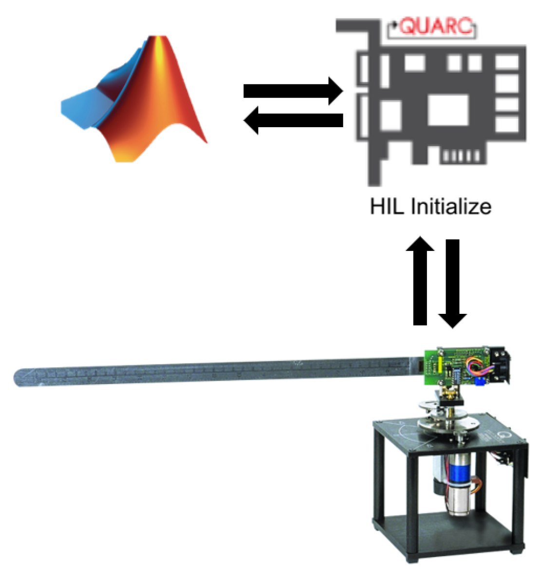
The rotary flexible link (RFL) system consists of a rotary servo motor coupled with a flexible steel link, serving as a model for lightweight robotic manipulators and cantilever beam structures. The servo angle ($\theta$) is measured through an incremental encoder, while a strain gauge captures the link deflection ($\alpha$). Data acquisition and communication are conducted via Simulink^®, version R2022B and the QUARC interface, version 2.15, as depicted in Figure 1 [37] and Figure 2.

The system identification process involves applying a square wave voltage to the motor and capturing the corresponding responses of $\theta$ and $\alpha$. Key parameters considered include the time vector (t), motor voltage (u), servo angle ($\theta$), and link deflection ($\alpha$). The controller is designed to ensure precise reference trajectory tracking while minimizing vibrations, maintaining operation within voltage constraints of $\pm 10$ V and a deflection range of $[-5^{\circ },5^{\circ }]$.

2.2. Experimental Setup

All experiments in this study were conducted using the QLabs Virtual Rotary Flexible Link platform, a high-fidelity digital twin of the physical Quanser Rotary Flexible Link hardware [38]. According to Quanser, the virtual platform is dynamically accurate and replicates the behavior of the physical hardware, making it suitable for rigorous experimentation in vibration suppression, system identification, and optimal control [39,40]. It allows full instrumentation and control through MATLAB/Simulink, version R2022B and provides the same model-based lab experience as the real-world system, except for the presence of physical sensor noise and cable disturbances, which are inherently absent in the virtual environment [38].

Table 1. Physical parameters of the flexible link [40].

Property	Value
Material	Stainless Steel
Total length	48 cm
Effective length (to strain gage)	41.9 cm
Link Mass	0.065 kg
Moment of inertia	0.0038 kg·m2
Strain gage range	±5 V
Strain gage sensitivity	1/16.5 rad/V

summarizes the physical parameters of the flexible beam emulated by the virtual model. These parameters are used in both modeling and control stages and represent the mechanical configuration of the hardware platform used in typical experimental labs.

The system used in this study is the QLabs Virtual Rotary Flexible Link; it consists of a rotary base driven by a servo motor, a flexible stainless-steel link, and calibrated sensors capable of accurately measuring the base angle and the tip deflection. To evaluate control performance, a full-state linear quadratic regulator (LQR) was implemented based on a four-state state-space model identified from virtual system data.

Table 2. LQR implementation capabilities of the QLabs Virtual System [39].

Aspect	Details
Control objective	Servo angle tracking and vibration minimization
Feedback type	Full-state feedback (4 states)
Simulation environment	Simulink + QUARC Real-Time
Platform used	QLabs Virtual Rotary Flexible Link
LQR computation	lqr(sys,Q,R) in MATLAB
Sampling time	0.002 s
Sensor interface	Incremental encoder and strain gage

details the simulation and implementation setup.

2.3. State Definition and Identification Procedure

The rotary flexible link system is modeled as a linear state-space system with four states, one input, and two outputs. The input is the motor voltage $V_m$, and the measured outputs are the servo angle $\theta$ and the relative deflection angle of the flexible link $\alpha$.

The four states of the system are defined as follows:

• $x_1=\theta$: angular position of the servo (rad);
• $x_2=\alpha$: relative angular deflection of the flexible link (rad);
• $x_3=\dot{\theta }$: angular velocity of the servo (rad/s);
• $x_4=\dot{\alpha }$: angular velocity of the flexible link deflection (rad/s).

These states describe the coupled dynamics of the underactuated rotary base and flexible link mechanism.

The identification process followed these detailed steps:

• Experimental Setup:The experiment was conducted using the QLabs Virtual Rotary Flexible Link platform, which, according to Quanser documentation, faithfully replicates the behavior of the physical hardware [40,41]. Proper initial conditions were ensured by starting from a non-vibrating position and avoiding cable interference.
• Input Signal: A square wave voltage was applied to the motor to sufficiently excite the dynamics of both the servo and the flexible link.
• Data Acquisition: The servo angle was measured using an incremental encoder, and the flexible link deflection was measured using a calibrated strain gauge. The data were recorded with a sampling time of 2 ms and stored in MATLAB variables.
• Dataset Preparation: The recorded data were organized into an iddata object.
• Model Estimation: A fourth-order state-space model was estimated using the ssest function from MATLAB’s System Identification Toolbox [42]. This function employs an iterative prediction error minimization algorithm to fit the model to the measured data.

2.4. Use of the ssest Function in System Identification

The ssest function, part of MATLAB’s System Identification Toolbox [43], is a robust and widely validated tool for estimating state-space models using time-domain or frequency-domain data [42]. It relies on an iterative prediction error minimization algorithm, which fine-tunes model parameters to best represent the dynamic behavior of the system [44]. Furthermore, the ability to initialize the estimation with known model structures enhances its adaptability to incorporate prior system knowledge [45].

2.5. System Identification Validation

The validation dataset, sourced from Quanser, corresponds to an RFL plant connected to a data acquisition (DAQ) card. The system features a 10V servo motor equipped with an incremental encoder offering a resolution of 4096 counts per revolution, alongside a strain gauge for deflection measurement. Data acquisition is carried out through the “Quanser Interactive Labs” platform (version 2.15) and processed via QUARC Real-Time Control Software [41]. This high-fidelity dataset enables the construction of an accurate state-space model, which is validated through open-loop response analysis, comparison of measured and simulated data, residual autocorrelation analysis, cross-correlation, and cross-validation [46,47,48,49].

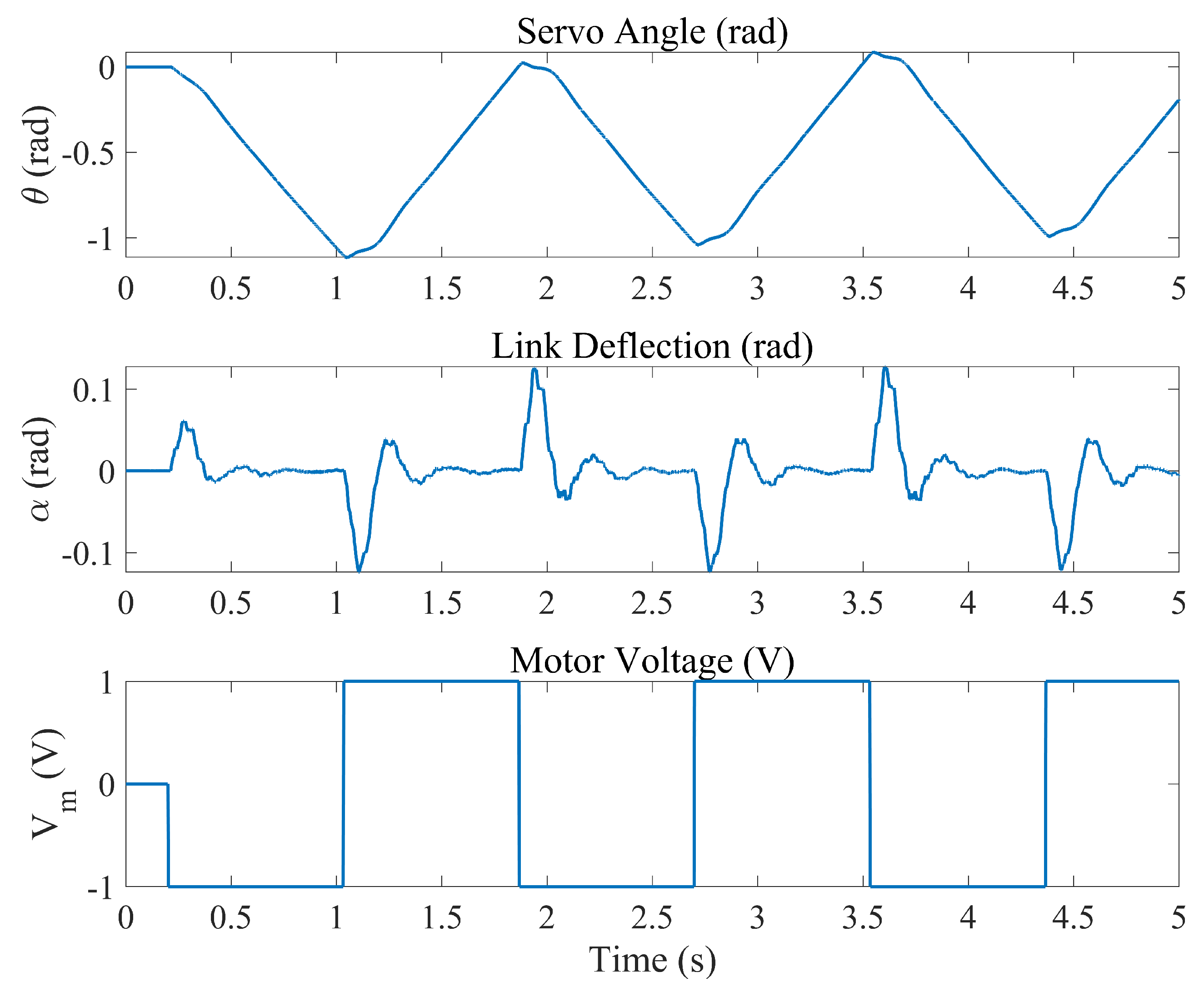
The obtained data are presented in a series of graphs showing the open-loop response of the system. Figure 3 shows the temporal evolution of the servo angle, link deflection, and the applied motor voltage.

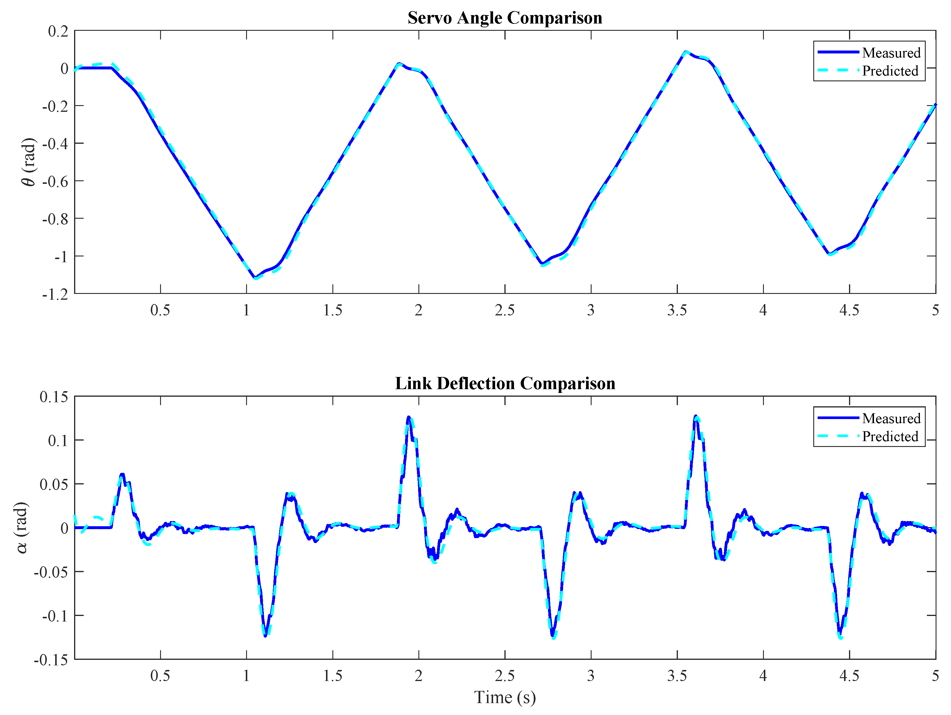
The comparison between the measured results and the simulations provided by the model, Figure 4, was performed using the compare command.

The auto-correlation of the residuals was calculated to assess the model’s sufficiency in capturing the system’s dynamics [50]. While the residuals for the servo angle output showed behavior close to white noise, indicating a good fit, the residuals for the link deflection exhibited some significant auto-correlations, suggesting areas for future model improvements (Figure 5).

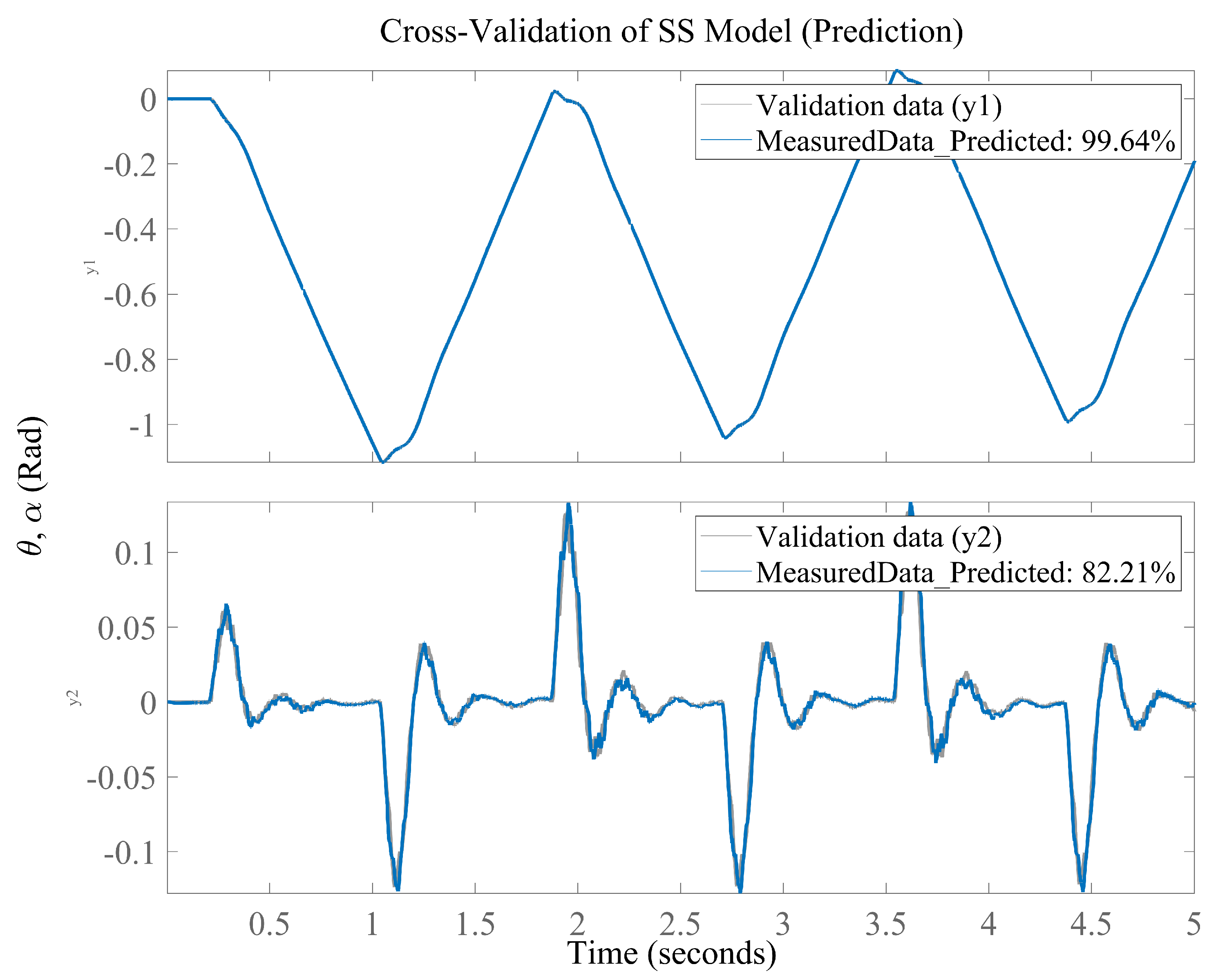
Through cross-validation, the predictions generated by the model are compared with the actual measured data, providing a critical assessment of the model’s ability to generalize to new data not used during the identification process [51]. The results visualized in Figure 6 demonstrate a high degree of agreement between the predictions and the real observations, particularly in tracking the servo angle ($\theta$), suggesting that the model accurately captures the system’s primary dynamics. However, the figure also reveals areas for improvement, as evidenced by the slight discrepancies observed in the prediction of the link deflection ($\alpha$).

To assess how well the identified model replicates the experimental system behavior, several standard quantitative metrics have been computed. These metrics are widely accepted in the system identification and control literature for evaluating model accuracy, predictive capability, and response fidelity.

Table 3. Quantitative evaluation metrics for model validation.

Metric	$\mathit{\theta }$ (Base)	$\mathit{\alpha }$ (Tip)	Desirable Ranges
RMSE (%)	1.1846	4.9196	<5%
MAE (%)	0.9298	3.4012	<5%
$R^2$ (coefficient of determination)	0.9986	0.9654	≥0.90
Willmott’s concordance index	0.9997	0.9921	≥0.90
IAE ($\int \left|e\right(t\left)\right|dt$)	0.0518	0.0217	As low as possible
ISE ($\int e^2\left(t\right)dt$)	0.00087	0.00020	As low as possible

summarizes the results and compares them to generally accepted thresholds or desirable ranges for model validation.

2.6. State-Space Model

The state-space model used in this work is defined as:

$$\begin{array}{cc}\hfill {\displaystyle \frac{dx\left(t\right)}{dt}}& =Ax\left(t\right)+Bu\left(t\right)\hfill \end{array}$$

(1)

$$\begin{array}{cc}\hfill y\left(t\right)& =Cx\left(t\right)+Du\left(t\right)\hfill \end{array}$$

(2)

where the state vector is given by:  

$$x\left(t\right)=\left[\begin{array}{c}{\theta }_{\mathrm{base}}\left(t\right)\\ {\alpha }_{\mathrm{link}}\left(t\right)\\ {\dot{\theta }}_{\mathrm{base}}\left(t\right)\\ {\dot{\alpha }}_{\mathrm{tip}}\left(t\right)\end{array}\right]$$

(3)

The matrices obtained via experimental identification are:

$$\mathbf{A}=\left[\begin{array}{cccc}0.2629& -0.6923& 2.055& 1.013\\ -11.52& 23.99& -54.79& -30\\ -4.291& -10.42& -63.96& -20.63\\ -3.471& 77.02& 24.48& -10.19\end{array}\right]$$

(4)

$$\mathbf{B}=\left[\begin{array}{c}-0.05998\\ 1.608\\ 7.151\\ -6.666\end{array}\right]$$

(5)

$$\mathbf{C}=\left[\begin{array}{cccc}29.62& 0.706& 0.1893& 0.134\\ -0.151& 0.8635& -0.7005& -0.5094\end{array}\right]$$

(6)

$$\mathbf{D}=\left[\begin{array}{c}0\\ 0\end{array}\right]$$

(7)

Equations (1) and (2) represent the standard form of the state-space system. In this case:

the matrix A defines the internal dynamics of the system;

the matrix B describes how the input (motor voltage) affects the states;

the matrix C defines the relationship between the states and the measured outputs (servo position and tip deflection);

the matrix D is null, which is typical when there is no direct feedthrough between input and output.

The matrices A, B, C, and D were obtained through the experimental identification process using the ssest function of the MATLAB System Identification Toolbox, based on measured data in the Quanser Virtual Flexible Link environment. This process is documented in the technical manuals of Quanser [40], and in the methodology applied in this study following [39].

The analysis of

Table 4. Parameterization and estimation details of the SS model.

Detail	Value
Parameterization type	FREE form (all coefficients free)
Feedthrough	None
Disturbance component	Estimate
Number of free coefficients	36
Software tools	idssdata, getpvec, getcov
Estimation method	SSEST
Data source	“MeasuredData”
Fit to data	$[99.85\%,96.95\%]$
FPE	$2.89\times {10}^{-13}$
MSE	$1.326\times {10}^{-6}$

reveals that a free-form parameterization with 36 coefficients and no feedthrough component was used, estimating disturbances from measured data. Specific tools (idssdata, getpvec, getcov) and the SSEST method were employed, achieving a highly accurate fit (ranging from 96.95% to 99.85%) with exceptionally low errors (FPE and MSE).

2.7. Theoretical Model

The complete theoretical derivation of the rotary flexible link system’s dynamic model, including the formulation based on Euler–Bernoulli beam theory, the application of Hamilton’s principle, the use of generalized coordinates, and the modal decomposition into a state-space representation, has been thoroughly developed in our previous work [52].

That article presents both the mechatronic modeling of the system and the analysis of its natural and forced vibration modes, laying the foundational framework for the design and evaluation of robust and tracking control strategies. The resulting model captures the kinetic energy contributions from both the motor and the flexible link, the bending potential energy, and the dynamic relationship between the applied motor torque and the angular response of the system. Additionally, it identifies the experimentally relevant vibrational modes for control applications.

For the sake of continuity, only the essential equations required to link the previous theoretical development with the experimental identification and controller validation proposed in this study are presented here. For full derivations involving boundary conditions, Laplace transforms, motion equations, and the final state-space model, the reader is referred to [52].

$$\left[\begin{array}{c}\dot{\theta }\\ \dot{\alpha }\\ \ddot{\theta }\\ \ddot{\alpha }\end{array}\right]=\left[\begin{array}{cccc}0& 0& 1& 0\\ 0& 0& 0& 1\\ 0& -{\displaystyle \frac{K_{\mathrm{stiff}}}{I_{\mathrm{base}}}}& -{\displaystyle \frac{K_T{K}_b{K}_g^2}{I_{\mathrm{base}}R}}& 0\\ 0& -K_{\mathrm{stiff}}\left({\displaystyle \frac{1}{I_T}}+{\displaystyle \frac{1}{I_{\mathrm{base}}}}\right)& -{\displaystyle \frac{K_T{K}_b{K}_g^2}{I_{\mathrm{base}}R}}& 0\end{array}\right]\left[\begin{array}{c}\theta \\ \alpha \\ \dot{\theta }\\ \dot{\alpha }\end{array}\right]+\left[\begin{array}{c}0\\ 0\\ {\displaystyle \frac{K_T{K}_g}{I_{\mathrm{base}}R}}\\ -{\displaystyle \frac{K_T{K}_g}{I_{\mathrm{base}}R}}\end{array}\right]V_a$$

(8)

$$C=\left[\begin{array}{cccc}1& 0& 0& 0\\ 0& 1& 0& 0\end{array}\right],D=\left[\begin{array}{c}0\\ 0\end{array}\right]$$

(9)

The experimental modal parameters that characterize the vibrational response of the system have also been previously identified.

Table 5. Frequencies of vibration modes in open loop. Adapted from [52].

Mode	Open Loop (Hz)
0 *	0
1	5.4245
2	3.7937

* Rigid-body mode.

summarizes the open-loop vibration frequencies, emphasizing the dominant modes relevant to controller design. These values support the validity of a reduced order single degree of freedom approximation under controlled conditions and are consistent with the findings reported in [52].

The vibrational response of the rotary flexible link system is characterized by the presence of both rigid-body motion and flexible link deformation. In open-loop conditions, the system exhibits distinct resonance modes, primarily dominated by the first two vibrational frequencies, as reported in Table 5. These modes correspond to the elastic dynamics of the flexible link and are critical for control design, as they determine the system’s tendency to oscillate in response to external torques. The first vibrational mode, around 5.42 Hz, represents the fundamental elastic deformation of the link, while the second mode at 3.79 Hz suggests a higher-order interaction potentially influenced by boundary effects and damping. The identification and characterization of these frequencies allow for targeted suppression strategies using state-feedback control.

The proposed GRL-LQR control methodology combines the reliability of optimal control with the adaptability of deep reinforcement learning. Initially, a LQR controller is used to provide structured reference signals, guiding the learning process and accelerating convergence. As training progresses, control authority gradually shifts from the LQR to the TD3 agent, allowing the policy to autonomously refine its behavior while preserving stability.

2.8. Using an Internal LQR Controller for the Initial Training Phase

To guide the agent’s learning in the early stages of training, an LQR controller was implemented in the system’s inner loop. This controller acted as a “behavioral baseline”, allowing the agent to observe a controlled response in terms of stability and accuracy across both output variables, even though it did not fully meet the desired control objectives. The LQR served as a preliminary stabilization mechanism to reduce initial oscillations and prevent extreme actions that could interfere with learning in the initial iterations. This initial “assisted learning” approach enabled the agent to begin adjusting its policy based on a relatively stable dynamic, decreasing the risk of instability during early exploration.

2.9. Internal Mechanisms of TD3 for Flexible-Link Control

The agent used in this study incorporates three key mechanisms, such as flexible-link mechanisms: (i) a twin critic architecture that mitigates overestimation bias by taking the minimum of two Q-value estimates; (ii) delayed policy updates, which enhance training stability by updating the actor less frequently than the critics; and (iii) target policy smoothing through Gaussian noise, which regularizes learning and improves generalization. Additionally, the LQR-guided training process imposes a stabilizing structure on the learned policy.

2.10. Reward Function

The reward function is designed to achieve two simultaneous objectives: accurate tracking of the base angle and minimization of tip oscillations. It is defined as:

$$\mathcal{R}\left(t\right)=\left\{\begin{array}{cc}-{\lambda }_T\left|x_1\left(t\right)-c_i\right|,\hfill & \mathrm{if}t<t_d,\hfill \\ R_T\left(t\right)+R_O\left(t\right),\hfill & \mathrm{if}t\ge t_d,\hfill \end{array}\right.$$

(10)

Here, $c_i$ denotes the initial reference (before the step), and $c_f$ the final reference (after the step). The step reference is applied at time $t_d$, and ${\lambda }_T$ is a weight that penalizes tracking error before the step is applied.

For $t\ge t_d$, the reward $\mathcal{R}\left(t\right)$ is composed of two components:

• Tracking reward $R_T\left(t\right)$:

The tracking error is defined as:

$$e_T\left(t\right)=\left|x_1\left(t\right)-c_f\right|.$$

(11)

If the tracking error is within a predefined settling band $B_B$, a positive reward proportional to the remaining margin is given:

$$R_T\left(t\right)={\lambda }_T(B_B-e_T\left(t\right)).$$

(12)

Otherwise, a penalty is applied:

$$R_T\left(t\right)=-{\lambda }_T{e}_T\left(t\right).$$

(13)

2.

Oscillation penalty $R_O\left(t\right)$:

Tip oscillation is defined by:

$$O\left(t\right)=\left|x_2\left(t\right)\right|,$$

(14)

where $x_2$ corresponds to the tip angular deflection. If $O\left(t\right)$ exceeds a defined tolerance $B_T$, the agent is penalized:

$$R_O\left(t\right)=-{\lambda }_O(O\left(t\right)-B_T).$$

(15)

Otherwise, a small bonus is given to encourage stability:

$$R_O\left(t\right)={\lambda }_O^{\prime }(B_T-O\left(t\right)).$$

(16)

Here, ${\lambda }_O$ is the penalty weight for excessive oscillation, and ${\lambda }_O^{\prime }$ is a smaller bonus weight for low oscillations.

Thus, the complete reward after $t\ge t_d$ is:

$$\mathcal{R}\left(t\right)=R_T\left(t\right)+R_O\left(t\right).$$

(17)

This formulation differentiates between the pre-reference activation phase ($t<t_d$) and the post-activation phase ($t\ge t_d$), penalizing anticipatory deviations from the initial reference $c_i$ and, once the reference changes to $c_f$, emphasizing accurate tracking of the new target while suppressing excessive tip oscillations. The parameters ${\lambda }_T$, ${\lambda }_O$, ${\lambda }_O^{\prime }$, $B_B$, and $B_T$ can be tuned to reflect the desired control objectives.

2.11. System Architecture and Network Design

Table 6. TD3 training and agent parameters.

Parameter	Value
Sample time	0.001 s
Experience buffer length	500,000
Discount factor	0.95
Mini batch size	256
Max episodes	200
Max steps per episode	$\lceil T_f/T_s\rceil$
Stop training criteria	Average Reward
Stop training value	200
Score averaging window length	100
Actor network learning rate	$5\times {10}^{-4}$
Critic network learning rate	$1\times {10}^{-2}$
Exploration model standard deviation	0.9
Exploration model decay rate	$1\times {10}^{-3}$
Exploration model minimum std.	0.91
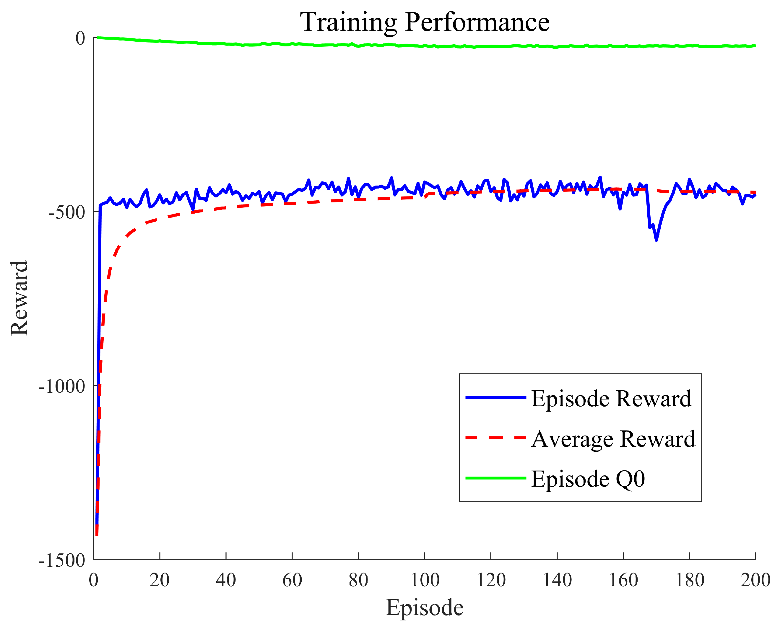
Use parallel training	No

summarizes the configuration parameters used in training the reinforcement learning agent using the twin delayed deep deterministic policy gradient (TD3) algorithm. The discount factor ($\gamma =0.95$) prioritizes long-term performance, while the mini-batch size of 256 provides a stable gradient estimation during updates. The training proceeds over a maximum of 200 episodes, each with a fixed step budget defined by the total simulation time $T_f$ and the sample time $T_s$. Training stops early when the average reward over the last 100 episodes surpasses a threshold of 200, reflecting satisfactory performance.

The actor and critic networks are trained using learning rates of $5\times {10}^{-4}$ and $1\times {10}^{-2}$, respectively. These values reflect the necessity for conservative policy updates (actor) and faster value estimation convergence (critic). The exploration model incorporates Gaussian noise with a standard deviation of 0.9, which decays at a rate of $1\times {10}^{-3}$ until a minimum threshold of 0.91 is reached, ensuring continued exploration while avoiding excessive variability in the control policy.

3. Problem Formulation

3.1. Control Objectives and System Constraints

The main objective of this study is to develop a controller capable of tracking a desired trajectory at the base of a rotary flexible-link system while actively suppressing tip vibrations. This problem is particularly challenging due to the underactuated and oscillatory nature of flexible structures, which tend to amplify disturbances and delay stabilization.

A significant constraint arises from the limited sensory information: the angular deflection at the tip ($\alpha$) is not directly measurable. Instead, strain gauges are placed at the base of the link, providing indirect observations of the system’s deformation. This lack of direct measurement complicates precise damping of vibrations, especially under fast or abrupt reference inputs. Therefore, the control strategy must rely on partial state information and learn to infer relevant dynamics during execution.

3.2. Guided Reinforcement-Learning Framework

Reinforcement-learning (RL) algorithms such as the twin delayed deep deterministic policy gradient (TD3) have shown promise in continuous control tasks due to their ability to learn policies in complex, nonlinear environments. However, standard RL approaches often face critical limitations, including:

• Slow convergence: High-dimensional problems require extensive interaction to learn optimal policies [53].
• High computational cost: Continuous updates to actor and multiple critic networks lead to intensive training [54].
• Inefficient exploration: Suboptimal exploration strategies increase training time and reduce policy robustness [55].

To address these limitations, this work adopts a guided reinforcement-learning (GRL) strategy. In this framework, the RL agent is initialized with a baseline policy derived from a classical linear quadratic regulator (LQR), which provides structure and stability during early learning. This hybrid guidance accelerates convergence, reduces variance in early episodes, and ensures that the learned policy remains within a region of safe and stable behavior [30].

Figure 7 illustrates the GRL workflow, which begins with system modeling and knowledge integration, followed by policy optimization and real-world deployment. The inclusion of prior control knowledge enhances learning stability across multiple stages of the pipeline.

4. Training Process

The training process (Figure 8) of the GRL–TD3 agent demonstrates a rapid and stable convergence. During the process, the agent was able to learn a robust control policy in just 200 episodes, highlighting the effectiveness of the initial guidance provided by the LQR controller in accelerating the learning process. This guided-learning strategy reduced random exploration and focused the training on optimizing reference tracking.

The episode reward curves and average reward exhibited consistent improvement, leading to reduced tracking error and enhanced overall performance. The stabilization of the Episode $Q_0$ metric suggests a reduction in Q-value estimation bias, contributing to learning stability. Furthermore, the reward function effectively balanced base tracking accuracy with acceptable tip oscillations, while well-optimized hyperparameters—including mini-batch size, experience buffer length, learning rates, and discount factor—significantly accelerated convergence.

Training Process of the GRL–TD3 Agent (Summary)

The GRL–TD3 agent was trained within a Simulink environment based on a state-space model obtained through experimental system identification of a flexible manipulator. Utilizing the TD3 algorithm, the agent maps state observations, including base angular position, angular velocity, and tip deformation to continuous torque actions, with a reward function designed to penalize tracking errors and excessive oscillations.

An internal LQR controller provides initial guidance, accelerating convergence by offering baseline control references. Over successive episodes, the initially dispersed trajectories of the base and tip oscillations gradually stabilize as the agent refines its policy through a replay buffer and a progressively decreasing Gaussian noise exploration strategy (Figure 9).

5. Evaluation of the GRL–TD3 Control Results

5.1. Step Response Analysis of GRL–TD3 Controllers

During training, critical parameters such as settling time, overshoot, and steady-state error for both output variables were evaluated. Iterative adjustments were made to the reward function and the maximum number of steps per episode to allow the agent to complete each simulation within an appropriate timeframe and maximize its learning in each episode.

The system’s response is compared to the response generated by an LQR controller. In Figure 10, the response of the base position to a step signal is compared due to the LQR control and the GRL–TD3 control. The GRL–TD3 and LQR controllers both stabilize the system close to the reference value within a similar timeframe. Notably, the response of the GRL–TD3 controller aligns more closely to the reference value slightly faster than the LQR. The steady-state error for the GRL–TD3 controller ($\pm 0.0318\%$) is significantly lower than that of the LQR ($\pm 6.2657\%$). Furthermore, the transition response of the GRL–TD3 controller is smoother, exhibiting no signs of oscillations or instabilities.

In Figure 11, the GRL–TD3 response (Blue) reaches the equilibrium position faster and exhibits significantly lower oscillation compared to LQR. The peak of the oscillation is 0.6875°, and the amplitude of these oscillations quickly decreases, stabilizing the tip at a position close to zero degrees. In contrast, the LQR response (Red) shows more pronounced oscillation that persists longer before stabilizing with a maximum oscillation peak of 2.3974°. The oscillations are of greater amplitude compared to GRL–TD3 and take longer to diminish, suggesting lesser effectiveness in managing the system dynamics.

Despite its initially more abrupt oscillation, the GRL–TD3 controller achieves more effective control in reducing the amplitude of subsequent oscillations more quickly than LQR. This improvement is due to the parameter adjustments in learning and adapting to the system’s dynamics.

The stabilization time was approximately two seconds longer than that of the LQR, and the reduction in reference error and improvement in overall stability allowed the TD3 agent to outperform the LQR in meeting multiple objectives, as shown in Figure 10 and Figure 11 and in

Table 7. Comparison of the system dynamics (link base) against proposed controllers.

Parameter	GRL–TD3	LQR
Settling time (s)	7.838	4.854
Overshoot (%)	0	0
Rise time (s)	4.332	2.686
Peak (°)	0.99403	0.93747
Peak time (s)	14.298	9.338
Steady state value (%)	0.50	6.25

and

Table 8. Comparison of system dynamics (link tip) against proposed controllers.

Parameter	GRL–TD3	LQR
Rise time (s)	0.2	0.002
Peak (°)	0.016306	0.039933
Peak time (s)	0.108	0.07
Steady state value (°)	−0.0032371	−0.007148

.

Table 9. Quantitative performance metrics for GRL–TD3 and LQR controllers.

Metric	$\mathit{\theta }$ (GRL–TD3)	$\mathit{\theta }$ (LQR)	$\mathit{\alpha }$ (GRL–TD3)	$\mathit{\alpha }$ (LQR)
RMSE (%)	20.02	23.72	6.94	7.66
MAE (%)	11.91	11.03	2.60	4.65
$R^2$ (coefficient of determination)	0.1561	−0.1848	−0.0581	−0.2945
Willmott’s concordance index	0.8183	0.7670	0.0743	0.1561
IAE ($\int \left|e\right(t\left)\right|dt$)	273.07	252.73	2.30	1.86
ISE ($\int e^2\left(t\right)dt$)	10,526.90	14,779.42	1.8885	0.4667

presents the quantitative performance metrics obtained for both the GRL–TD3 and LQR controllers, evaluated for the base angle ($\theta$) and the tip deflection ($\alpha$). The table includes standard error metrics such as RMSE and MAE expressed as percentages, along with statistical indicators like the coefficient of determination ($R^2$) and Willmott’s concordance index. Additionally, integral performance measures are reported through the integral of absolute error (IAE) and the integral of squared error (ISE), providing a cumulative assessment of tracking error over time. Each metric is calculated independently for both variables of interest, enabling a direct numerical comparison between the two control strategies.

5.2. Stability Assessment of the Learned Policy

Since the TD3 controller operates in a model-free setting, classical stability analysis based on pole placement or Lyapunov functions is not directly applicable. Instead, we adopt an empirical boundedness criterion to assess external stability, consistent with the BIBO (bounded-input bounded-output) definition. Specifically, the system output is considered externally stable if the response remains within a finite and proportional range relative to the reference signal over time. This approach is commonly employed in the evaluation of learned controllers where only input-output data are available, and no analytical model is accessible [56].

In our analysis, the output $\theta$ was monitored to ensure that it remained bounded with respect to the reference, using a threshold set at twice the steady-state value. No divergence or sustained growth was detected in the trajectories under either controller. This supports the conclusion that both LQR and GRL–TD3 policies yielded externally stable behavior over the test horizon.

5.3. Comparative Analysis of Control Systems on a Rotatory Flexible Link

The following comprehensive comparison, presented in

Table 10. Comparison of system dynamics for additional controllers [52].

Features	Fuzzy	NN	GA–LQR	LQR	GRL–TD3
Settling time (s)	>60	9	4.5	4.8	7.83
Peak (°)	0.0573	0.0573	0.0216	0.0400	0.0163

, involves various control systems applied to a rotatory flexible link system. This analysis evaluates two main variables: stabilization time and the dynamics at the tip of the flexible link for four different controllers: fuzzy, neural network (NN) [57], GA–LQR [52], LQR, and the proposed GRL–TD3 controller. Significant differences in their settling times and peak magnitudes are highlighted, emphasizing each controller’s capabilities and limitations in dynamic response.

The controllers exhibit notable differences in response speed and tip oscillation peaks. GA–LQR (0.45 s) and LQR (0.7 s) stabilize rapidly, enabling immediate corrections, whereas the fuzzy controller, with a settling time exceeding 60 s, is more suitable for precision-demanding tasks. The neural network controller balances speed and control with a response time of 9 s, while the proposed GRL–TD3 achieves stabilization in 7.83 s, offering a versatile solution.

Regarding tip oscillations, GA–LQR maintains a low peak of 0.0216° for smooth control, whereas LQR exhibits a higher peak of 0.0400°. Both the fuzzy and neural network controllers present moderate peaks of 0.0573°. Notably, GRL–TD3 outperforms all others, achieving the smallest oscillation peak of 0.016306°, demonstrating superior oscillation suppression and enhanced stability.

6. Parameter Uncertainty Analysis and Robustness Evaluation

Reinforcement learning (RL) has shown promising advancements in control applications; however, given that a general theory of stability and performance in the RL domain has not yet been established, it is essential to conduct exhaustive and rigorous testing of the controller prior to implementation. This ensures that potential instabilities and performance degradation are identified before deployment [58].

In order to evaluate the robustness of the GRL–TD3 control system, a parameter uncertainty analysis was performed by applying $\pm 30\%$ offsets to the nominal gains of the LQR controller. This approach simulates variations in the plant model and allows for an assessment of the closed-loop system’s sensitivity to parameter deviations. The uncertainties are visualized using polar plots, the nominal gain for each channel is represented as a reference orbit (highlighted in red), with the perturbed gains distributed around it (see Figure 12). Although the angular coordinates in these plots do not carry direct physical significance, they serve as a convenient means to illustrate the magnitude and directional bias of the variations. This methodology is well supported by robust control theory [59] and multivariable feedback control principles [60], both of which advocate the inclusion of parametric uncertainties in controller design to ensure robust performance. Moreover, recent studies in reinforcement learning for control have demonstrated that guided exploration using an expert controller such as the LQR to steer the learning process can accelerate convergence and enhance robustness, thereby justifying the GRL–TD3 framework.

6.1. Experimental Setup and Performance Metrics

To evaluate the robustness of the GRL–TD3 control system, an experimental campaign was conducted comprising 16 simulations. In each simulation, a unique offset was added to the nominal gain vector of the LQR controller, resulting in a modified gain matrix expressed as

$$K_{\mathrm{total}}=K_{\mathrm{nom}}+k_{\mathrm{offset}},$$

where each element of $k_{\mathrm{offset}}$ was perturbed by up to $\pm 30\%$ of its nominal value. The objective was to assess the system’s robustness to parametric uncertainty by observing the closed-loop response to both a step reference and a periodic reference with variable amplitude. Performance was evaluated using metrics such as the relative error (%) which quantifies the deviation between the actual response and the desired reference and a performance index that summarizes the overall behavior of the system. In the polar plots (see Figure 12), the parameter variations are clearly observed, represented by the gain values in the K matrix.

Figure 13 shows the simulation results for the LQR controller. Although the controller maintains closed-loop stability across all 16 simulations, its robustness, measured by performance, is not consistently achieved. Specifically, while the tip response is attenuated, the base response fails to reliably track the reference signal under the evaluated parametric uncertainties. This disparity suggests that, despite the LQR’s ability to stabilize the system, its performance deteriorates under significant gain variations, highlighting a gap between mere stability and robust performance.

In Figure 14, the simulation results for the GRL–TD3 controller are illustrated. The base position trajectories converge very closely to the reference signal, exhibiting only a minor steady-state error, which indicates effective tracking performance. Concurrently, the tip of the flexible link displays controlled oscillations, which are a direct consequence of the reward function designed to balance the performance between base tracking and tip regulation. Compared to the conventional LQR controller, the GRL–TD3 approach not only achieves a more uniform clustering of the base responses in steady state but also realizes a slight reduction in the maximum tip oscillations. This demonstrates that the guided reinforcement-learning strategy successfully enhances overall robustness by mitigating excessive tip movement while maintaining precise base control.

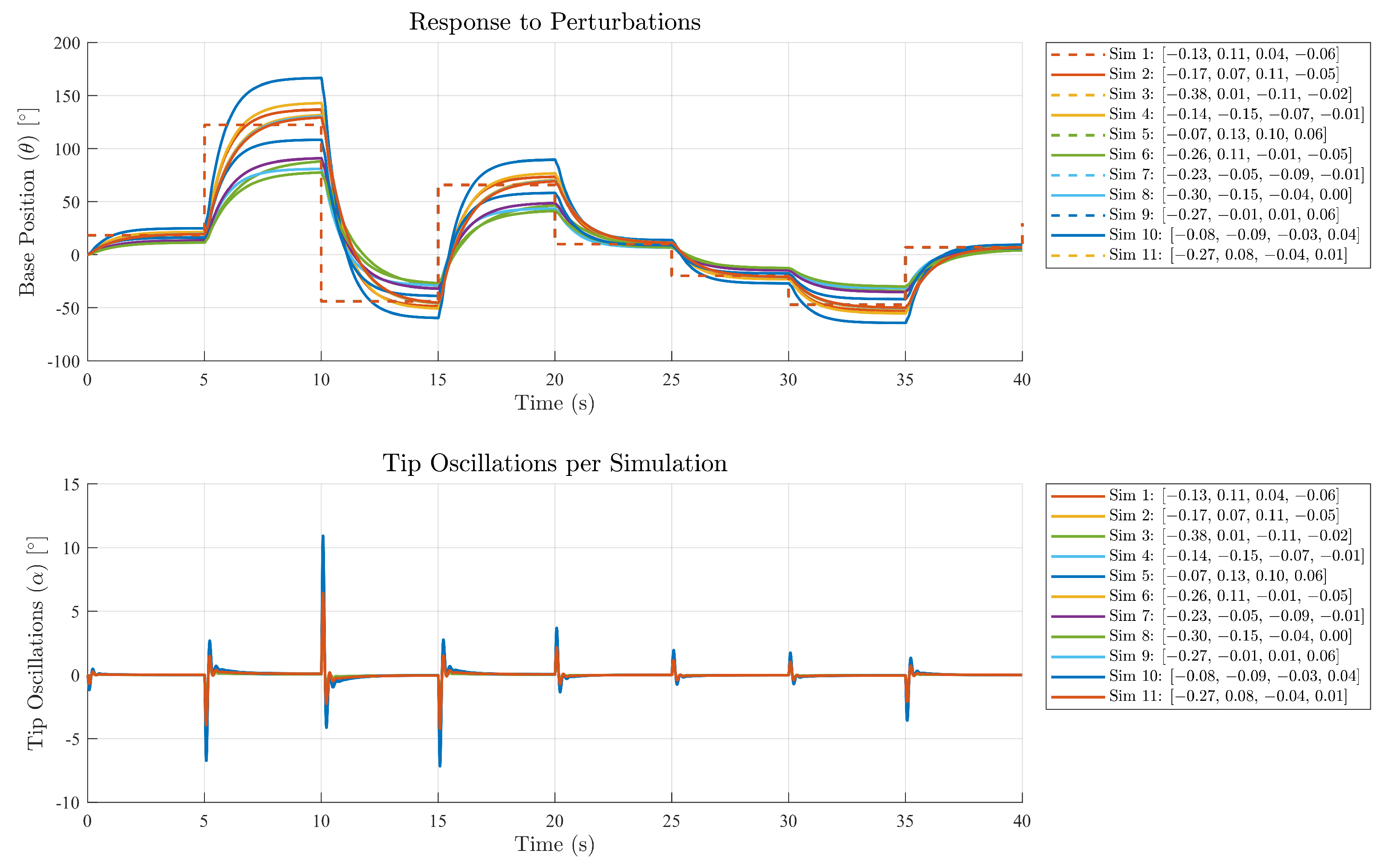
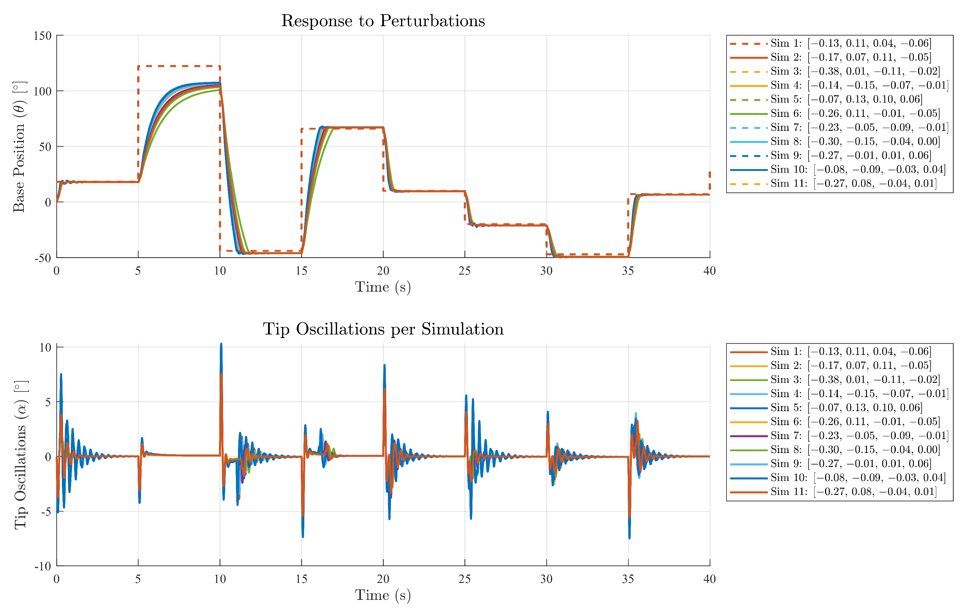
6.2. Performance Evaluation of the LQR Under a Periodic Input of Variable Amplitude

Figure 15 illustrates the response of the system, controlled using an LQR, to a periodic input with variable amplitude. The graph reveals that, in most experiments, the base response does not reach the desired reference, indicating a lack of robustness in the LQR controller. Moreover, during abrupt or large changes in the reference signal, the resulting oscillations can reach up to 10 degrees.

6.3. Response of the GRL–TD3 Controlled System

In Figure 16, the simulation results using the GRL–TD3 controller are shown. In this case, the system successfully reaches the desired reference, demonstrating that the control strategy not only meets the tracking requirements but is also capable of significantly reducing oscillations, even in the presence of the complex flexible dynamics of the link. Although some oscillations are observed at the tip, they remain at very low levels since the controller prioritizes precise tracking of the base position. This behavior is crucial in real-world applications, where minimizing tip oscillations is essential to ensure system stability and accuracy.

6.4. Analysis of Excluded Simulations and Robustness of the GRL–TD3 Controller

Out of the 16 simulations performed, five (specifically, simulations 1, 4, 7, 9, and 14) were excluded due to instability issues. This instability arises because the uncertainty parameters, particularly the offset applied to $k_1$, are around the critical value of 1. In the polar plot, these simulations cluster around the orbit with a radius of 1, indicating that values near this threshold lead to closed-loop instability or critical stability of the system. This behavior demonstrates that, within a defined robustness margin, the GRL–TD3 controller can effectively track the base reference even under substantial disturbances.

It is noteworthy that, as a reinforcement-learning-based control system, the GRL–TD3 controller has learned to prioritize accurate tracking of the base position, even if that entails permitting slightly larger oscillations at the tip. This approach is consistent with the designed reward function, which heavily penalizes both oscillations and tracking errors of the base. In scenarios where the parameter variations are excessive, it may be necessary to adjust or redesign the reward function to achieve a more balanced trade-off between reducing oscillations and maintaining precise reference tracking.

6.5. Comparative Analysis of LQR and GRL–TD3 Controllers Under Parametric Uncertainty

Table 11. LQR controller results.

Simulation	k11	k22	k33	k44	Relative Error Percent	Performance Score
1	0.13183	−0.011333	0.020657	−0.059544	5.7752	94.225
2	−0.13344	0.11285	0.039999	−0.058782	12.096	87.904
3	−0.16545	0.069495	0.11091	−0.054971	17.211	82.789
4	0.36533	0.035785	−0.069487	−0.0622	8.4181	91.582
5	−0.37781	0.0075371	−0.11089	−0.016193	26.721	73.279
6	−0.14002	−0.15247	−0.068786	−0.01243	33.668	66.332
7	0.22574	−0.089573	0.049242	−0.063679	10.25	89.75
8	−0.067397	0.13082	0.09777	0.064049	36.325	63.675
9	0.28758	0.010565	0.085774	−0.013965	6.6262	93.374
10	−0.26253	0.11467	−0.010186	−0.047168	8.4703	91.53
11	−0.23059	−0.049063	−0.088685	−0.013012	25.287	74.713
12	−0.29867	−0.15448	−0.04223	0.0038678	35.985	64.015
13	−0.2681	−0.012506	0.0050516	0.058336	7.4662	92.534
14	0.24821	−0.10443	−0.072677	−0.048352	21.059	78.941
15	−0.081101	−0.089413	−0.025884	0.035313	11.215	88.785
16	−0.26667	0.079369	−0.041524	0.0077923	6.5444	93.456

presents the outcomes of the system controlled by a conventional LQR approach under varying parametric offsets. Each simulation corresponds to a different offset applied to the baseline gains ($k_{11},k_{22},k_{33},k_{44}$), reflecting the plant’s sensitivity to uncertain dynamics. Notably, while the LQR controller ensures nominal stability in most cases, the relative error percent (RE) and performance score (PS) vary considerably. The more substantial RE values (e.g., simulations 6, 8, and 12) highlight the limitations of relying solely on an LQR scheme for robust performance. This underscores the need for advanced control or learning-based techniques when the plant experiences significant parameter fluctuations, especially in highly flexible or underactuated systems.

Table 12. GRL–TD3 controller results.

Simulation	k11	k22	k33	k44	Relative Error Percent	Performance Score
1	0.13183	−0.011333	0.020657	−0.059544	4.9515	95.048
2	−0.13344	0.11285	0.039999	−0.058782	6.7966	93.203
3	−0.16545	0.069495	0.11091	−0.054971	7.1133	92.887
4	0.36533	0.035785	−0.069487	−0.0622	4.0058	95.994
5	−0.37781	0.0075371	−0.11089	−0.016193	10.505	89.495
6	−0.14002	−0.15247	−0.068786	−0.01243	6.8345	93.165
7	0.22574	−0.089573	0.049242	−0.063679	4.5156	95.484
8	−0.067397	0.13082	0.09777	0.064049	6.2222	93.778
9	0.28758	0.010565	0.085774	−0.013965	4.2771	95.723
10	−0.26253	0.11467	−0.010186	−0.047168	8.3251	91.675
11	−0.23059	−0.049063	−0.088685	−0.013012	7.8639	92.136
12	−0.29867	−0.15448	−0.04223	0.0038678	8.8643	91.136
13	−0.2681	−0.012506	0.0050516	0.058336	8.3932	91.607
14	0.24821	−0.10443	−0.072677	−0.048352	4.4225	95.577
15	−0.081101	−0.089413	−0.025884	0.035313	6.3136	93.686
16	−0.26667	0.079369	−0.041524	0.0077923	8.3824	91.618

illustrates how the guided reinforcement-learning (GRL–TD3) controller, specifically the GRL–TD3 approach, adapts to the same set of parametric variations used in the LQR tests. Despite facing the same uncertain conditions, the relative error percent is generally lower, and the performance score is consistently higher or comparable across most simulations These results validate the premise that a learning-based controller, guided by an expert policy (LQR in this case), can effectively mitigate performance degradation induced by model uncertainty.

The comparative table (

Table 13. Comparative results: percentage improvement between LQR and GRL controllers.

Sim	LQR RE (%)	GRL RE (%)	RE Improvement (%)	LQR PS	GRL PS	PS Improvement (%)
1	5.78	4.95	14.26	94.23	95.05	0.87
2	12.10	6.80	43.83	87.90	93.20	6.03
3	17.21	7.11	58.63	82.79	92.89	12.19
4	8.42	4.01	52.38	91.58	96.00	4.81
5	26.72	10.51	60.73	73.28	89.50	22.15
6	33.67	6.83	79.66	66.33	93.17	40.42
7	10.25	4.52	55.93	89.75	95.48	6.39
8	36.33	6.22	82.81	63.68	93.78	47.27
9	6.63	4.28	35.44	93.37	95.72	2.52
10	8.47	8.33	1.71	91.53	91.68	0.16
11	25.29	7.86	68.87	74.71	92.14	23.32
12	35.99	8.86	75.33	64.02	91.14	42.38
13	7.47	8.39	−12.42	92.53	91.61	−1.00
14	21.06	4.42	78.98	78.94	95.58	21.08
15	11.22	6.31	43.70	88.79	93.69	5.52
16	6.54	8.38	−28.10	93.46	91.62	−1.97

) quantifies the relative error (RE) and performance score (PS) improvements achieved by the GRL-based controller over the classical LQR approach. A positive RE improvement reflects a reduction in tracking error, and a positive PS improvement denotes enhanced overall performance. Most simulations (e.g., 2, 3, 4, 7, 8) show substantial gains, frequently exceeding 50% in RE improvement, underlining the robustness of the learned controller in coping with uncertain parameters. Nonetheless, a few simulations (e.g., 13, 16) demonstrate negative improvement, revealing that while GRL generally outperforms LQR, certain parameter offsets can challenge the controller’s learned policy. These findings highlight the importance of thorough parameter studies, reward function refinement, and potentially hybrid robust-learning designs to consistently ensure performance across a broad range of operational scenarios.

7. Discussion and Future Work

This study demonstrated that integrating a linear quadratic regulator (LQR) with a twin delayed deep deterministic policy gradient (TD3) agent via guided reinforcement learning (GRL–TD3) enhances control performance and robustness in rotary flexible link systems. The LQR component ensures initial stability and accelerates convergence, while TD3 adapts to dynamic variations and learns effective control strategies. Despite these benefits, the methodology remains sensitive to reward design, hyperparameter tuning, and lacks interpretability posing challenges for certification and safety-critical deployment.

The analysis adopted an empirical BIBO–based criterion to evaluate external stability, given that classical model-based approaches are not directly applicable to learned policies. Monitoring the output trajectory confirmed that the GRL–TD3 controller produced bounded responses across all test scenarios. Nonetheless, the absence of formal guarantees highlights the need for further research into theoretical stability analysis and certification frameworks for reinforcement-learning-based controllers.

As the approach has only been validated in a simulation environment, future work should focus on real-world implementation. Practical deployment may involve unmodeled phenomena such as friction, backlash, and sensor delays, which could affect performance. Experimental validation on physical platforms is necessary to assess robustness under these conditions and confirm the applicability of the controller in real settings.

The lightweight architecture of the trained policy makes it suitable for embedded real-time applications. Prior research has shown that deep RL policies can be executed efficiently on microcontrollers using techniques such as quantization and hardware acceleration [61,62,63]. Deploying the trained actor on embedded systems while offloading training to external platforms offers a feasible path for industrial implementation.

A further research direction involves evaluating the controller’s robustness to structural variations (e.g., link stiffness, damping), which were not explored here due to the fixed configuration of the experimental platform. This would extend the current framework toward transferable or adaptive policies applicable across families of flexible mechanisms.

8. Conclusions

This work presented a hybrid control methodology that combines a linear quadratic regulator (LQR) with a twin delayed deep deterministic policy gradient (TD3) agent, using guided reinforcement learning (GRL–TD3) to control a rotary flexible link system. The approach leverages the stability guarantees of classical control and the adaptability of reinforcement learning to achieve robust trajectory tracking while mitigating oscillations at the flexible link’s tip.

Simulation-based experiments confirmed that the integration of LQR guidance during TD3 training accelerates convergence, constrains unsafe exploration, and enhances the overall robustness of the learned policy. The learned controller achieved stable and bounded performance under a range of operating conditions. However, the architecture remains sensitive to reward shaping and hyperparameter selection, which directly influence learning quality and final performance.

Future work should aim at validating the approach on physical hardware, incorporating adaptive mechanisms, and exploring policy transfer to structurally similar systems. Moreover, efforts to phase out or adapt the expert LQR guidance over time could foster greater policy autonomy while retaining stability. This research highlights the potential of GRL–TD3 as a versatile solution for controlling flexible robotic systems and opens avenues for broader application in real-world scenarios requiring both precision and robustness.

References

1. Subedi, D.; Tyapin, I.; Hovland, G. Review on Modeling and Control of Flexible Link Manipulators. Model. Identif. Control 2020, 41, 141–163. [Google Scholar] [CrossRef]
2. Mansour, T.; Konno, A.; Uchiyama, M. Modified PID Control of a Single-Link Flexible Robot. Adv. Robot. 2012, 22, 433–449. [Google Scholar] [CrossRef]
3. Reher, J.; Csomay-Shanklin, N.; Christensen, D.L.; Bristow, B.; Ames, A.D.; Smoot, L.S. Passive Dynamic Balancing and Walking in Actuated Environments. In Proceedings of the 2020 IEEE International Conference on Robotics and Automation (ICRA), Paris, France, 31 May–31 August 2020. [Google Scholar] [CrossRef]
4. Ma, P.; Xia, R.; Wang, X.; Zhang, X.; Królczyk, G.; Gardoni, P.; Li, Z. An active control method for vibration reduction of a single-link flexible manipulator. J. Low Freq. Noise Vib. Act. Control 2022, 41, 1497–1506. [Google Scholar] [CrossRef]
5. Kronander, K.; Billard, A. Passive Interaction Control With Dynamical Systems. IEEE Robot. Autom. Lett. 2015, 1, 106–113. [Google Scholar] [CrossRef]
6. Ebrahimi, A.; Heydari, M.; Alasty, A. Active control of a passive bipedal walking robot. Int. J. Dyn. Control 2017, 5, 733–740. [Google Scholar] [CrossRef]
7. Solak, G.; Ajoudani, A. Online Learning and Suppression of Vibration in Collaborative Robots with Power Tools. In Proceedings of the 2023 IEEE International Conference on Robotics and Automation (ICRA), London, UK, 29 May–2 June 2023. [Google Scholar] [CrossRef]
8. Bächer, M.; Hoshyari, S.; Xu, H.; Coros, S.; Knoop, L.E. Computational Vibration Suppression for Robotic Systems. U.S. Patent US 2020/0406461 A1, 31 December 2020. [Google Scholar]
9. Guo, C.; Yi, J. Vibration Suppression Control in Robotic Percussive Drilling. In Proceedings of the American Control Conference 2018, Milwaukee, WI, USA, 27–29 June 2018. [Google Scholar] [CrossRef]
10. Investigating the Potential of Flexible Links for Increased Payload to Mass Ratios for Collaborative Robotics. IEEE Access 2022, 11, 15981–15995. [CrossRef]
11. Raju, E.M.; Krishna, L.S.R.; Abbas, M. Control of End-Effector of a Multi-link Robot with Joint and Link Flexibility. In Recent Trends in Mechanical Engineering, Proceedings of the ICIME 2019, London, UK, 19–21 September 2019; Springer: Berlin/Heidelberg, Germany, 2020. [Google Scholar] [CrossRef]
12. Yao, Z.; Liang, X.; Jiang, G.P.; Yao, J. Model-Based Reinforcement Learning Control of Electrohydraulic Position Servo Systems. IEEE/ASME Trans. Mechatron. 2023, 28, 1446–1455. [Google Scholar] [CrossRef]
13. Pinosky, A.; Abraham, I.; Broad, A.; Argall, B.; Murphey, T.D. Hybrid control for combining model-based and model-free reinforcement learning. Int. J. Robot. Res. 2023, 42, 337–355. [Google Scholar] [CrossRef]
14. Zielinski, K.M.; Hendges, L.V.; Florindo, J.B.; Lopes, Y.K.; Ribeiro, R.; Teixeira, M.; Casanova, D. Flexible control of Discrete Event Systems using environment simulation and Reinforcement Learning. Appl. Soft Comput. 2021, 111, 107714. [Google Scholar] [CrossRef]
15. Raoufi, M.; Delavari, H. Designing a Model-Free Reinforcement Learning Controller for a Flexible-Link Manipulator. In Proceedings of the 2021 9th RSI International Conference on Robotics and Mechatronics (ICRoM), Tehran, Iran, 17–19 November 2021; pp. 1–6. [Google Scholar] [CrossRef]
16. Rahimi, F.; Ziaei, S.; Esfanjani, R.M. A Reinforcement Learning-Based Control Approach for Tracking Problem of a Class of Nonlinear Systems: Applied to a Single-Link Manipulator. In Proceedings of the 2023 31st International Conference on Electrical Engineering (ICEE), Tehran, Iran, 9–11 May 2023; pp. 58–63. [Google Scholar] [CrossRef]
17. Shahid, A.A.; Roveda, L.; Piga, D.; Braghin, F. Learning Continuous Control Actions for Robotic Grasping with Reinforcement Learning. In Proceedings of the 2020 IEEE International Conference on Systems, Man, and Cybernetics (SMC), Toronto, ON, Canada, 11–14 October 2020; pp. 4066–4072. [Google Scholar] [CrossRef]
18. Char, I.; Schneider, J. PID-Inspired Inductive Biases for Deep Reinforcement Learning in Partially Observable Control Tasks. arXiv 2023, arXiv:2307.05891. [Google Scholar]
19. Pierallini, M.; Angelini, F.; Mengacci, R.; Palleschi, A.; Bicchi, A.; Garabini, M. Trajectory Tracking of a One-Link Flexible Arm via Iterative Learning Control. In Proceedings of the 2020 IEEE/RSJ International Conference on Intelligent Robots and Systems (IROS), Las Vegas, NV, USA, 25–29 October 2020; pp. 7579–7586. [Google Scholar] [CrossRef]
20. Lin, M.; Sun, Z.; Xia, Y.; Zhang, J. Reinforcement Learning-Based Model Predictive Control for Discrete-Time Systems. IEEE Trans. Neural Netw. Learn. Syst. 2023, 35, 3312–3324. [Google Scholar] [CrossRef] [PubMed]
21. Zhang, S.; Sun, C.; Feng, Z.; Hu, G. Trajectory-Tracking Control of Robotic Systems via Deep Reinforcement Learning. In Proceedings of the 2019 IEEE International Conference on Cybernetics and Intelligent Systems (CIS) and IEEE Conference on Robotics, Automation and Mechatronics (RAM), Bangkok, Thailand, 18–20 November 2019; pp. 386–391. [Google Scholar] [CrossRef]
22. Viswanadhapalli, J.K.; Elumalai, V.K.; Shivram, S.; Shah, S.; Mahajan, D. Deep reinforcement learning with reward shaping for tracking control and vibration suppression of flexible link manipulator. Appl. Soft Comput. 2024, 152, 110756. [Google Scholar] [CrossRef]
23. Zhu, J.; Tang, W. Design of Intelligent Controller for Aero-engine Based on TD3 Algorithm. Inf. Technol. Control 2023, 52, 1010–1024. [Google Scholar] [CrossRef]
24. Fan, J.; Dou, D.; Ji, Y.; Liu, N.; Chen, S.W.; Yan, H.; Li, J. Two-Loop Acceleration Autopilot Design and Analysis Based on TD3 Strategy. Int. J. Aerosp. Eng. 2023, 2023, 5759135. [Google Scholar] [CrossRef]
25. Egbomwan, O.E.; Liu, S.; Chaoui, H. Twin Delayed Deep Deterministic Policy Gradient (TD3) Based Virtual Inertia Control for Inverter-Interfacing DGs in Microgrids. IEEE Syst. J. 2023, 17, 2122–2132. [Google Scholar] [CrossRef]
26. Yazar, O.; Coskun, S.; Li, L.; Zhang, F.; Huang, C. Actor-Critic TD3-based Deep Reinforcement Learning for Energy Management Strategy of HEV. In Proceedings of the 2023 5th International Congress on Human-Computer Interaction, Optimization and Robotic Applications (HORA), Istanbul, Turkey, 8–10 June 2023. [Google Scholar] [CrossRef]
27. Gu, Y.; Zhu, Z.; Lv, J.; Wang, X.; Xu, S. D3-TD3: Deep Dense Dueling Architectures in TD3 Algorithm for Robot Path Planning Based on 3D Point Cloud. J. Circuits Syst. Comput. 2023, 32, 2350305. [Google Scholar] [CrossRef]
28. Cai, Y.; Zhang, C.; Zhao, L.; Shen, W.; Zhang, X.; Song, L.; Bian, J.; Qin, T.; Liu, T. TD3 with Reverse KL Regularizer for Offline Reinforcement Learning from Mixed Datasets. In Proceedings of the 2022 IEEE International Conference on Data Mining (ICDM), Orlando, FL, USA, 28 Novermber–1 December 2022. [Google Scholar] [CrossRef]
29. Zhu, X.; Zhu, X.; Chen, J.; Zhang, S.; Nan, B.; Bi, L. Learning of Quadruped Robot Motor Skills Based on Policy Constrained TD3. In Proceedings of the Chinese Automation Congress (CAC), Chongqing, China, 17–19 November 2023. [Google Scholar]
30. Eßer, J.; Bach, N.; Jestel, C.; Urbann, O.; Kerner, S. Guided Reinforcement Learning: A Review and Evaluation for Efficient and Effective Real-World Robotics [Survey]. IEEE Robot. Autom. Mag. 2023, 30, 67–85. [Google Scholar] [CrossRef]
31. Duan, H.; Dao, J.; Green, K.; Apgar, T.; Fern, A.; Hurst, J. Learning Task Space Actions for Bipedal Locomotion. In Proceedings of the 2021 IEEE International Conference on Robotics and Automation (ICRA), Xi’an, China, 30 May–5 June 2021; pp. 1276–1282. [Google Scholar] [CrossRef]
32. Wong, J.; Makoviychuk, V.; Anandkumar, A.; Zhu, Y. OSCAR: Data-driven operational space control for adaptive and robust robot manipulation. In Proceedings of the 2022 International Conference on Robotics and Automation (ICRA), Philadelphia, PA, USA, 19–23 May 2022; pp. 10519–10526. [Google Scholar]
33. Gheni, E.; Al-Khafaji, H.; Alwan, H. A deep reinforcement learning framework to modify LQR for an active vibration control applied to 2D building models. Open Eng. 2024, 14, 20220496. [Google Scholar] [CrossRef]
34. Ouyang, Y.; He, W.; Li, X. Reinforcement learning control of a single-link flexible robotic manipulator. IET Control Theory Appl. 2017, 11, 1426–1433. [Google Scholar] [CrossRef]
35. Qiu, Z.C.; Chen, G.H.; Zhang, X.M. Trajectory planning and vibration control of a translational flexible hinged plate based on optimization and reinforcement learning algorithm. Mech. Syst. Signal Process. 2022, 179, 109362. [Google Scholar] [CrossRef]
36. Anayi, F.; Packianather, M.; Samad, B.; Yahya, K. Simulating LQR and PID Controllers to Stabilise a Three-Link Robotic System. In Proceedings of the 2022 2nd International Conference on Advance Computing and Innovative Technologies in Engineering, Greater Noida, India, 28–29 April 2022; pp. 2033–2036. [Google Scholar]
37. Quanser. Quanser Interactive Labs for Distance & Blended Control Systems and Robotics Courses. 2024. Available online: https://www.quanser.com/products/rotary-flexible-link/ (accessed on 12 January 2024).
38. Quanser. QLabs Virtual Rotary Flexible Link Data Sheet; High-Fidelity Digital Twin of the Rotary Flexible Link Platform; Internal Technical Documentation; Quanser: Markham, ON, Canada, 2020. [Google Scholar]
39. Quanser. Rotary Flexible Link System Identification and LQR Design. 2025. Available online: https://www.mathworks.com/matlabcentral/fileexchange/103605-rotary-flexible-link-system-identification-and-lqr-design (accessed on 10 May 2025).
40. Quanser. Rotary Flexible Link Data Sheet; Internal Technical Documentation Provided by Manufacturer; Quanser: Markham, ON, Canada, 2025. [Google Scholar]
41. Quanser. QLabs Virtual Rotary Flexible Link. Virtual Laboratory Platform. 2025. Available online: https://www.quanser.com/products/qlabs-virtual-rotary-flexible-link/ (accessed on 15 December 2024).
42. MathWorks. System Identification Toolbox—ssest Function. 2022. Available online: https://www.mathworks.com/help/ident/ref/ssest.html (accessed on 15 December 2024).
43. MathWorks. System Identification Toolbox—MATLAB. 2023. Available online: https://www.mathworks.com/products/sysid.html (accessed on 10 May 2025).
44. MathWorks. State-Space Model Estimation Methods. 2022. Available online: https://www.mathworks.com/help/ident/ug/state-space-model-estimation-methods.html (accessed on 10 May 2025).
45. MathWorks. How to Use Multiple Input-Output Datasets in Ssest Function (MIMO). 2023. Available online: https://www.mathworks.com/matlabcentral/answers/2056481 (accessed on 10 May 2025).
46. Gao, F.; Li, J.; Sun, G. Efficient and accurate flexible multibody dynamics modeling for complex spacecraft with integrated control applications. Acta Astronaut. 2024, 219, 818–825. [Google Scholar] [CrossRef]
47. Murray-Smith, D.J. Measures of Quality for Model Validation. In Testing and Validation of Computer Simulation Models; Springer: Cham, Switzerland, 2014. [Google Scholar] [CrossRef]
48. Ljung, L. Chapter 13: Frequency domain methods and FRF estimation. In System Identification: Theory for the User, 2nd ed.; Prentice Hall: Englewood Cliffs, NJ, USA, 1999. [Google Scholar]
49. Trzęsiok, M. Measuring the Quality of Multivariate Statistical Models. Acta Univ. Lodz. Folia Oeconomica 2019, 6, 99–100. [Google Scholar] [CrossRef]
50. Korner-Nievergelt, F.; Roth, T.; von Felten, S.; Guélat, J.; Almasi, B.; Korner-Nievergelt, P. Assessing Model Assumptions: Residual Analysis. In Bayesian Data Analysis in Ecology Using Linear Models with R, BUGS, and STAN; Academic Press: Cambridge, MA, USA, 2014. [Google Scholar] [CrossRef]
51. Brown, D.A. Model Selection Through Cross-Validation for Supervised Learning Tasks with Manifold Data. J. Purdue Undergrad. Res. 2024, 13, 41. [Google Scholar] [CrossRef]
52. Saldaña Enderica, C.A.; Llata, J.R.; Torre-Ferrero, C. Optimization of Q and R Matrices with Genetic Algorithms to Reduce Oscillations in a Rotary Flexible Link System. Robotics 2024, 13, 84. [Google Scholar] [CrossRef]
53. Andrychowicz, M. Hindsight experience replay. In Advances in Neural Information Processing Systems 2017; MIT Press: Cambridge, MA, USA, 2017; pp. 5048–5058. [Google Scholar]
54. Arulkumaran, K.; Deisenroth, M.P.; Brundage, M.; Bharath, A.A. Deep reinforcement learning: A brief survey. IEEE Signal Process. Mag. 2017, 34, 26–38. [Google Scholar] [CrossRef]
55. Bacon, P.L.; Harb, J.; Precup, D. The option-critic architecture. Proc. Aaai Conf. Artif. Intell. 2017, 31, 1726–1734. [Google Scholar] [CrossRef]
56. Khalil, H.K. Nonlinear Systems, 3rd ed.; Prentice Hall: Englewood Cliffs, NJ, USA, 2002. [Google Scholar]
57. López, J.C. Control of a Single-Link Flexible Manipulator. Master’s Thesis, University of Cantabria, Santander, Spain, 2022. Available online: https://repositorio.unican.es/xmlui/handle/10902/24745 (accessed on 16 December 2024).
58. Schenke, M.; Wallscheid, O. A Deep Q-Learning Direct Torque Controller for Permanent Magnet Synchronous Motors. IEEE Open J. Ind. Electron. Soc. 2021, 2, 232–243. [Google Scholar] [CrossRef]
59. Zhou, K.; Doyle, J.C.; Glover, K. Robust and Optimal Control; Prentice Hall: Upper Saddle River, NJ, USA, 1996. [Google Scholar]
60. Skogestad, S.; Postlethwaite, I. Multivariable Feedback Control: Analysis and Design; Wiley: Hoboken, NJ, USA, 2005. [Google Scholar]
61. Scheel, J.; Sarmiento, A.; Luca, M.; Peters, J. Real-time reinforcement learning for robotics without GPUs. arXiv 2020, arXiv:2009.11684. [Google Scholar]
62. Nagabandi, A.; Kahn, G.; Fearing, R.S.; Levine, S. Neural network dynamics for model-based deep reinforcement learning with model-free fine-tuning. In Proceedings of the 2018 IEEE International Conference on Robotics and Automation (ICRA), Brisbane, Australia, 21–25 May 2018; pp. 7559–7566. [Google Scholar]
63. Hwangbo, J.; Lee, J.; Dosovitskiy, A.; Bellicoso, D.; Tsounis, V.; Koltun, V.; Hutter, M. Learning agile and dynamic motor skills for legged robots. Sci. Robot. 2019, 4, eaau5872. [Google Scholar] [CrossRef]
Figure 1. Rotary flexible link communication (Quanser®, Markham, QC, Canada).
Robotics 14 00076 g001
Figure 2. Quanser Interactive Labs (Quanser®).
Robotics 14 00076 g002
Figure 3. Open loop response RFL.
Robotics 14 00076 g003
Figure 4. Comparison between the SS model and measured data.
Robotics 14 00076 g004
Figure 5. Auto-correlations.
Robotics 14 00076 g005
Figure 6. Cross-validation of SS model (prediction).
Robotics 14 00076 g006
Figure 7. Workflow of the guided reinforcement-learning (GRL) approach for robotic control optimization [30].
Robotics 14 00076 g007
Figure 8. Training performance.
Robotics 14 00076 g008
Figure 9. Training process of the reinforcement-learning-based controller for the flexible rotary system. Note: These curves represent the training process and not the final controller results.
Robotics 14 00076 g009
Figure 10. Response comparison–servo base.
Robotics 14 00076 g010
Figure 11. Response comparison–link tip.
Robotics 14 00076 g011
Figure 12. Stored final gains in polar coordinates.
Robotics 14 00076 g012
Figure 13. Simulation results for LQR controller.
Robotics 14 00076 g013
Figure 14. Simulation results for GRL–TD3 controller.
Robotics 14 00076 g014
Figure 15. Simulation results for using LQR controller.
Robotics 14 00076 g015
Figure 16. Simulation results for GRL–TD3 controller.
Robotics 14 00076 g016