H_∞ Control for Systems with Mechanical Constraints Based on Orthogonal Decomposition

Abstract

In this paper, we study $H_{\infty }$ control for systems with explicit mechanical constraints and a lack of state information, such as walking robots. This paper proposes an $H_{\infty }$ control design scheme based on solving an optimization problem with linear matrix inequality constraints. Our method is based on the orthogonal decomposition of the state variables and the use of two linear controllers and a Luenberger observer, tuned to achieve the desired properties of the closed-loop system. The method takes into account static linear additive disturbance, which appears due to the uncertainties associated with the mechanical constraints. We propose a dynamics linearization procedure for systems with mechanical constraints, taking into account the inevitable lack of information about the environment; this procedure allows a nonlinear system to be transformed into a form suitable for the application of the proposed control design method. The method is tested on a constrained underactuated three-link robot and a flat quadruped robot, showing the desired behavior in both cases.

1. Introduction

Legged robots have always been a focus of robotics research. Rapid progress over the last several years has led to the first instances of mass production of legged robots, as well as to the first cases of their practical use [1]. This in turn opens new questions, such as the reliability and robustness of legged robots and their control systems. In particular, one may pose the following questions: is it possible to design a control system for a legged robot that would be robust with respect to external disturbances, and is it possible to prove this property? In this paper, we aim to give a particular answer to these questions.

The progress achieved in legged robotics has been partially due to a successful adaptation of well-known control methods, such as Model-Predictive Control (MPC) [2,3], Proportional-Differential (PD) control, Extended Kalman Filters (EKFs) [4], and others. These methods in their standard formulations are directly applicable to systems like industrial robot arms; however, they require modifications to be used for legged robots. Legged robots acquire and break mechanical contact with the supporting surface as a part of their motion, leading to discontinuities in their models. Between discontinuous events (acquisition or breaking of contact), the dynamics of legged robots are well described via differential-algebraic equations (DAEs), where the mechanical constraints are explicitly stated. From the point of view of state estimation, it presents a qualitative difference from models with smooth dynamics described via ordinary differential equations (ODEs).

There are well-known robust control design methods: disturbance observer, adaptive control, quadratic stability, s-procedure-based robust control, etc. [5,6,7,8]. $H_{\infty }$ control is an especially promising type of robust control, as can be seen in recent advancements in the area [9,10,11,12]. In this work, we focus on $H_{\infty }$ control. Effective $H_{\infty }$ control design methods require the plant to be modeled as a system of linear ODEs, while legged robots are modeled with nonlinear DAEs.

Numerous methods can be used to transform a legged robot model into an ODE; these methods usually rely on differentiating constraint equations and introducing a change of variables [13,14,15]. Among these is the orthogonal decomposition method, which consists of projecting dynamics onto the null space of the constraints equations, while decomposing the state variables into the sets of static and independent states. This results in a system of independent ODEs with independent variables. In this paper, we discuss how this process can be combined with linearization to produce an accurate linear model. The resulting linear model can be used to derive $H_{\infty }$ control.

For practical legged robots, the full-state information is not available (some of the floating base states are usually not measured), requiring the use of observers or equivalent constructions. In this paper, we use the Luenberger state observer, adapting it to the model produced by the orthogonal decomposition method. To tune the controller and observer gains and ensure $H_{\infty }$ gain properties, we derive and solve a linear matrix inequality (LMI) condition. The systems where the controller and observer are tuned simultaneously produce bi-linear matrix inequalities (BMIs); to transform these into an LMI, we use Young’s relation, following an earlier example proposed in [5].

In this paper, we propose a control design method for constrained mechanical systems, finding the optimal gains for a linear controller and Luenberger observer in terms of the $H_{\infty }$ norm of the system, minimizing the system’s reaction to an external disturbance in terms of its $L_2$ norm. To our knowledge, this is the first $H_{\infty }$ control method designed to handle constrained mechanical systems with unmeasured static states. We present an LMI condition that guarantees the upper bound on the $H_{\infty }$ gain and that can be used directly in the optimal control design formulated as a semidefinite program (SDP). Our method allows us to account for additive terms in the model, related to the uncertainty in the constraints (or equivalently, the uncertainty in our knowledge about the environment in which the robot operates). To this end, we give a comprehensive description of a linearization method for dynamical systems with mechanical constraints, producing a linear model in the tangent space to the constraint manifold. We verify the results via numerical experiments on an underactuated three-link robot with a constrained end-effector and a flat quadruped model.

The remainder of the paper is organized as follows. In Section 2, we review the state of the art and discuss closely related works. Section 3 introduces the proposed linearization method for constrained systems. In Section 4, we provide definitions and formulas useful in the remaining sections. The mathematical formulation of the problem solved in this paper is given in Section 5, and in Section 6, we describe and prove the proposed solution to that problem. The last section provides a description of numeric experiments verifying the method.

2. State of the Art

The control system of a modern walking robot usually consists of multiple layers. The configuration and type of these layers vary significantly. A typical example would include a high-level trajectory and step planner, an MPC that runs over the pre-determined foothold positions, a QP-based feedback controller, and an array of motor-level PID controllers. This is augmented with an EKF-based state estimator and a simultaneous localization and mapping (SLAM) algorithm [2,16].

The control systems of the type described above use several simplified dynamical models of the robot. These include a point-mass model, a single rigid body (SRB) model (often with additional assumptions and simplifications), and a linear model that relates generalized accelerations to reaction forces and control inputs (but not the state) based on the full dynamical model evaluated at a single moment in time. The first of these is often used in the design of MPC, the second in EKF, and the last in QP-based feedback controllers [4,17].

Our goal is to propose a control system that guarantees robustness with respect to bounded-energy exogenous inputs. This motivates the decision to use the linearization of the full dynamics of the robot as our model and to simultaneously design both the controller and the observer, guaranteeing that the system’s $H_{\infty }$ gain is below the desired threshold. The linear model used to tune the proposed controller is required to be the optimal local linear approximation of the robot dynamics on the tangent space to the constraint manifold.

Previously, successful attempts to design optimal controllers and observers for systems with explicit contact constraints have been made [13,18,19]; we describe these works in the next subsection. However, the question of robustness to exogenous inputs has not been raised in those papers. In the area of optimal control, a similar (but more general) class of linear systems has been considered—descriptor systems [20]. For these systems, several robust control methods have been proposed [7]; we review them in Section 2.2.

2.1. Orthogonal Projection and Decomposition Methods

Orthogonal projection and decomposition (OPD) methods can be seen as an attempt to re-model the dynamics of systems with explicit constraints (presented as a DAE) into a form suitable for control design, using orthogonal projections and decomposition of the state variables.

An early example of such work can be found in [21], where orthogonal projections are used to exclude algebraic variables from equations of dynamics. Same as in most OPD methods, [21] takes advantage of a projector onto the null space of the constraint Jacobian. One of the key features of the work is the construction of a constraint inertia matrix—an analog to the generalized inertia matrix in Lagrangian mechanics. This approach is applied for solving problems related to simulation, inverse dynamics, and control design [21,22,23].

A parallel series of works proposed using QR decomposition of the constraint Jacobian and introduced a QR decomposition-based projector matrix [14,24,25,26]. They showed the equivalence of several independently developed OPD methods for inverse dynamics [25].

The works we have cited so far used an orthogonal projection of the dynamics equations to find a better representation of the relations between the generalized accelerations, control inputs, and reaction forces; as such, they were dealing with nonlinear second-order ODEs. A new class of methods originated in [13,18], where (1) a projection of the state variables (rather than the generalized accelerations) onto the tangent space of the constraint manifold was proposed and (2) a locally linearized model of the robot dynamics was considered. This allowed for the implementation of an LQR control for a walking robot.

In the paper [19], a decomposition of the state variables into active (lying on the tangent space to the constraint manifold) and static (orthogonal to the active ones) states was used to allow simultaneous controller and observer design, including a disturbance observer estimating the value of static state variables. This paper used the same linearized model as [18]. In [27,28], orthogonal decomposition was used to facilitate a simulation-based reinforcement learning algorithm on a constraint manifold.

While orthogonal projection and decomposition methods have successfully covered problems such as controller and observer design, as well as forward and inverse dynamics, there are still numerous control-related problems that have not been solved within this framework. One of them is the problem of designing a control law robust to an energy-bound exogenous input, which would guarantee a bounded output. This motivates the aim of the present paper: to design an $H_{\infty }$ controller–observer pair for the systems with explicit mechanical constraints, which can be represented by a linearized model in the tangent space to the constraint manifold. Additionally, we present a detailed treatment of the question of constructing linearized models, mentioned above, which has not been performed previously in OPD-related papers.

2.2. Linear Models for Constrained Systems

A descriptor system is a state-space model that expresses the relation between state variables and their derivatives in a general form, allowing the system to be described as a mix of differential and algebraic equations. The generality of such a description allows the systems with explicit mechanical constraints to be presented as descriptor systems. Descriptor systems have been extensively studied, and several important results have been achieved in the development of stability criteria as well as control and observer design methods [29]. The problem of designing an $H_{\infty }$ controller for a descriptor system was considered in [7,30], where a version of the Bounded Real Lemma was proposed, and in [31], where the Riccati equation was used to design an $H_{\infty }$ controller.

While these results are of significant interest, it has not been shown that a mechanical system with changing contact, such as a walking robot, can be successfully controlled using these methods. The class of descriptor systems is very general and includes far more than only systems with mechanical constraints; control methods designed for a smaller class of systems, such as OPD methods, can take advantage of the specific dynamic properties of the individual systems. For example, in [19], an OPD controller–observer design method allowed an unobservable system to be reduced to an observable one without the loss of information relevant to the control task.

Aside from the descriptor models, one can attempt the linearization of systems with explicit mechanical constraints based on Taylor expansion. The end result can be a model, linear with respect to the full state of the original nonlinear system, control actions, and reaction forces; we can call it an explicit form of a linear model with mechanical constraints. Alternatively, a model can be linearized on the tangent plane to the constraint manifold, producing a model with no reaction forces and a state vector of fewer dimensions; we can call it an implicit model. In papers [18,19], the transformation of an explicit model to an implicit one is discussed. In [13], the construction of a full-state implicit linear model is considered, while in [32], a linear model for floating-base coordinates (the position and orientation of the robot’s body and corresponding velocities) is constructed using an orthogonal projection of the nonlinear equations. In this paper, we extend and elaborate on this method, presenting a finite difference-based linearization scheme that produces models equivalent to the type required by OPD methods such as those proposed in [18].

3. Preliminaries

We start by recalling a few general results, which will be used in the following derivations.

Schur complement [33]: Given symmetric matrices $\mathbf{A}\in {\mathbb{S}}^n$ and $\mathbf{C}\in {\mathbb{S}}^m$ and a matrix $\mathbf{B}\in {\mathbb{R}}^{n\times m}$, as well as their concatenation

$$\begin{array}{c}\hfill \mathbf{M}=\left[\begin{array}{cc}\mathbf{A}& \mathbf{B}\\ {\mathbf{B}}^T& \mathbf{C}\end{array}\right],\end{array}$$

we can make the following equivalent statements:

• $\mathbf{M}<0$.
• $\mathbf{A}-\mathbf{B}{\mathbf{C}}^{-1}{\mathbf{B}}^T<0,\mathbf{C}<0$.

Here and later, the signs < and ≤ imply negative definiteness and semidefiniteness when applied to the matrices or quadratic forms (equivalently for the opposite sign).

Young’s Relation [33]: For any symmetric positive definite matrix $\mathbf{M}>0$, positive scalar $ϵ>0$, and $\mathbf{X},\mathbf{Y}\in {\mathbb{R}}^{n\times m}$, the following inequality is true:

$${\mathbf{X}}^T\mathbf{Y}+{\mathbf{Y}}^T\mathbf{X}\le {\mathbf{X}}^Tϵ{\mathbf{M}}^{-1}\mathbf{X}+{\displaystyle \frac{1}{ϵ}}{\mathbf{Y}}^T\mathbf{M}\mathbf{Y}.$$

(1)

$L_2$ Gain for Linear Systems [33]: Given an LTI system:

$$\left\{\begin{array}{c}\dot{\mathbf{x}}=\mathbf{A}\mathbf{x}+\mathbf{B}\mathbf{w},\hfill \\ \mathbf{z}=\mathbf{C}\mathbf{x}+\mathbf{D}\mathbf{w},\hfill \end{array}\right.$$

(2)

where $\mathbf{x}$, $\mathbf{z}$, and $\mathbf{w}$ are the system state, desired output vector, and the disturbance input, respectively, while $\mathbf{A}$, $\mathbf{B}$, $\mathbf{C}$, and $\mathbf{D}$ are the state, control, observation and feed-through matrices, respectively, we define its $L_2$ gain (which is also its $H_{\infty }$ norm) as:

$$\underset{{\left|\right|\mathbf{w}\left|\right|}_2\ne 0}{sup}{\displaystyle \frac{{\left|\right|\mathbf{z}\left|\right|}_2}{{\left|\right|\mathbf{w}\left|\right|}_2}},$$

(3)

where ${\left|\right|\mathbf{z}\left|\right|}_2$ is $L_2$ norm of the signal, defined as:

$${\left|\right|\mathbf{z}\left|\right|}_2^2={\int }_0^{\infty }\mathbf{z}{\left(t\right)}^T\mathbf{z}\left(t\right)dt,$$

(4)

and ${\left|\right|w\left|\right|}_2$ is defined equivalently. If there exists a function $V\left(\mathbf{x}\right)={\mathbf{x}}^T\mathbf{P}\mathbf{x}>0$ and the following equation holds for some scalar $\gamma >0$:

$$J=\dot{V}+{\displaystyle \frac{1}{\gamma }}{\mathbf{z}}^T\mathbf{z}-\gamma {\mathbf{w}}^T\mathbf{w}<0,$$

(5)

then the $H_{\infty }$ norm of the system is bounded by $\gamma$.

4. The Linearization of a Constrained Model

A walking robot can be modeled using a combination of Lagrange and constraint equations:

$$\left\{\begin{array}{c}{\mathbf{H}}_m\ddot{\mathbf{q}}+{\mathbf{C}}_m\dot{\mathbf{q}}+{\mathbf{g}}_m={\mathbf{S}}_m\tau +{\mathbf{J}}_m^T\lambda ,\hfill \\ {\mathbf{J}}_m\ddot{\mathbf{q}}+{\dot{\mathbf{J}}}_m\dot{\mathbf{q}}=0,\hfill \end{array}\right.$$

(6)

where ${\mathbf{H}}_m$, ${\mathbf{C}}_m$, ${\mathbf{g}}_m$, and ${\mathbf{J}}_m={\displaystyle \frac{\partial \mathbf{h}}{\partial \mathbf{q}}}$ are the generalized inertia matrix, Coriolis and normal inertial force matrix, generalized gravity force, and constraint Jacobian, while $\mathbf{q}$, $\lambda$, $\tau$, and ${\mathbf{S}}_m$ are generalized coordinates, reaction forces, joint torques, and an actuation selector matrix. The second equation is obtained by twice-differentiating the constraint equation ${\mathbf{h}}_m\left(\mathbf{q}\right)=0$.

These equations can be solved to find an explicit formula for the generalized accelerations:

$$\ddot{\mathbf{q}}={\psi }_m(\mathbf{q},\dot{\mathbf{q}},\tau )=(\mathbf{I}-{\mathbf{J}}_m^{\#}{\mathbf{J}}_m){\mathbf{H}}_m^{-1}({\mathbf{S}}_m\tau -{\mathbf{C}}_m\dot{\mathbf{q}}-{\mathbf{g}}_m)-{\mathbf{J}}_m^{\#}{\dot{\mathbf{J}}}_m{\dot{\mathbf{q}}}_m,$$

(7)

where ${\mathbf{J}}_m^{\#}={\mathbf{H}}_m^{-1}{\mathbf{J}}_m^T{\left({\mathbf{J}}_m{\mathbf{H}}_m^{-1}{\mathbf{J}}_m^T\right)}^{-1}$ is an inertially weighted pseudoinverse. We can describe the dynamics in a state-space form with state variables $\mathbf{q}$, $\dot{\mathbf{q}}$:

$$\begin{array}{c}\hfill {\displaystyle \frac{d}{dt}}\left[\begin{array}{c}\mathbf{q}\\ \dot{\mathbf{q}}\end{array}\right]=\left[\begin{array}{c}\dot{\mathbf{q}}\\ {\psi }_m(\mathbf{q},\dot{\mathbf{q}},\tau )\end{array}\right].\end{array}$$

(8)

Introducing state variable $\mathbf{x}={\left[\begin{array}{cc}{\mathbf{q}}^T& {\dot{\mathbf{q}}}^T\end{array}\right]}^T\in {\mathbb{R}}^n$ and control input $\mathbf{u}=\tau$, we re-write the last system as:

$$\begin{array}{c}\hfill \dot{\mathbf{x}}={\varphi }_m(\mathbf{x},\mathbf{u}).\end{array}$$

(9)

4.1. Orthogonal Decomposition of State Coordinates

The state-space model obtained above produces correct state derivatives, given states that correspond to the constraints. We use this model to produce a least-squares-type linearization scheme for the original constrained model. To this end, we need to identify variations $\Delta {\mathbf{x}}_i$ of the state variable $\mathbf{x}$ that do not leave the constraint manifold defined by the equation ${\mathbf{h}}_m\left(\mathbf{q}\right)=0$ and its derivative ${\mathbf{J}}_m\dot{\mathbf{q}}=0$. We consider the Taylor expansion of both equations around a point ${\mathbf{q}}_0$, ${\dot{\mathbf{q}}}_0$:

$$\begin{array}{cc}\hfill 0& ={\mathbf{h}}_m\left(\mathbf{q}\right)={\mathbf{h}}_m\left({\mathbf{q}}_0\right)+{\displaystyle \frac{\partial \mathbf{h}}{\partial \mathbf{q}}}(\mathbf{q}-{\mathbf{q}}_0)+\mathrm{h}.\mathrm{o}.\mathrm{t}.\hfill \\ \hfill 0& ={\mathbf{J}}_m\dot{\mathbf{q}}={\mathbf{J}}_m\left({\mathbf{q}}_0\right){\dot{\mathbf{q}}}_0+{\displaystyle \frac{\partial {\mathbf{J}}_m\dot{\mathbf{q}}}{\partial \mathbf{q}}}(\mathbf{q}-{\mathbf{q}}_0)+{\displaystyle \frac{\partial {\mathbf{J}}_m\dot{\mathbf{q}}}{\partial \dot{\mathbf{q}}}}(\dot{\mathbf{q}}-{\dot{\mathbf{q}}}_0)+\mathrm{h}.\mathrm{o}.\mathrm{t}.\hfill \end{array}$$

(10)

where higher-order terms (h.o.t.) include quadratic and higher-order terms in variables $\mathbf{q}$ and $\dot{\mathbf{q}}$ of the Taylor expansion. Since the linearization point lies on the constraint manifold, we cancel the terms ${\mathbf{h}}_m\left({\mathbf{q}}_0\right)=0$ and ${\mathbf{J}}_m\left({\mathbf{q}}_0\right){\dot{\mathbf{q}}}_0=0$. Introducing variations $\Delta \mathbf{q}=\mathbf{q}-{\mathbf{q}}_0$ and $\Delta \dot{\mathbf{q}}=\dot{\mathbf{q}}-{\dot{\mathbf{q}}}_0$ and dropping the higher-order terms, we obtain a linear system of equations governing the admissible values of variations:

$$\left[\begin{array}{cc}{\mathbf{J}}_m& 0\\ {\dot{\mathbf{J}}}_m& {\mathbf{J}}_m\end{array}\right]\left[\begin{array}{c}\Delta \mathbf{q}\\ \Delta \dot{\mathbf{q}}\end{array}\right]=\left[\begin{array}{c}0\\ 0\end{array}\right].$$

(11)

We denote the matrix on the left-hand side of the system as $\mathbf{G}$, obtaining conditions $\mathbf{G}\Delta {\mathbf{x}}_i=0$, with an implication that any admissible $\Delta {\mathbf{x}}_i$ lies in the null space of that matrix.

Let $\mathbf{N}\in {\mathbb{R}}^{n\times n_r}$ be an orthonormal basis in the null space of $\mathbf{G}$, and let $\mathbf{R}\in {\mathbb{R}}^{n\times n_{\rho }}$ be an orthonormal basis in its orthogonal compliment. Any vector $\mathbf{x}\in {\mathbb{R}}^n$ can be represented via its coordinates in the direct sum of the two subspaces:

$$\mathbf{x}=\mathbf{N}\mathbf{r}+\mathbf{R}\rho ,$$

(12)

where $\mathbf{r}$ are coordinates in the tangent plane to the constraint manifold, which we will call active states or null space coordinates, and $\rho$ are coordinates in the linear space that is normal to the manifold, which we will refer to as static states or a static state discrepancy. Since $\Delta {\mathbf{x}}_i$ lies entirely in the null space of $\mathbf{G}$, we can represent it via its null space coordinates $\Delta {\mathbf{r}}_i$ as $\Delta {\mathbf{x}}_i=\mathbf{N}\Delta {\mathbf{r}}_i$.

Note that by differentiating the constraints equation twice, we obtain a condition on the state derivative $\mathbf{G}\dot{\mathbf{x}}=0$. Then, any admissible state derivative $\dot{\mathbf{x}}$ can be expressed via its null space coordinates: $\dot{\mathbf{x}}=\mathbf{N}\dot{\mathbf{r}}$, and equivalently $\dot{\mathbf{r}}={\mathbf{N}}^T\dot{\mathbf{x}}={\mathbf{N}}^T{\varphi }_m(\mathbf{x},\mathbf{u})$. With that, we can construct linearized dynamics in the tangent plane to the constraint manifold.

Let ${\mathbf{E}}_r\in {\mathbb{R}}^{n_r\times n_r}$ be a full-rank matrix and ${\mathbf{e}}_i$ be its i-th column. Then, we can find an admissible state variation $\Delta {\mathbf{x}}_i=\mathbf{N}{\mathbf{e}}_i$; we denote the corresponding state derivative variation as:

$$\Delta {\mathbf{v}}_i={\mathbf{N}}^T\left({\varphi }_m({\mathbf{x}}_0+\mathbf{N}{\mathbf{e}}_i,{\mathbf{u}}_0)-{\varphi }_m({\mathbf{x}}_0,{\mathbf{u}}_0)\right).$$

(13)

Concatenating state derivatives into a matrix ${\mathbf{V}}_r=[\Delta {\mathbf{v}}_1,\dots \Delta {\mathbf{v}}_{n_r}]$, we obtain an active state matrix ${\mathbf{A}}_r$ of the linear model by finding the least-squares solution to the following system of equations:

$${\mathbf{V}}_r={\mathbf{A}}_r\mathbf{N}{\mathbf{E}}_r.$$

(14)

We find the control matrix $\mathbf{B}$ in a similar way, considering variations in control actions $\mathbf{u}$.

4.2. Constraint Uncertainty and the Static States

Assume that equation ${\mathbf{h}}_m\left(\mathbf{q}\right)=0$ and its derivative are augmented with a small additive term, which is uncertain. Then, expanding both equations around the point ${\mathbf{q}}_0$, ${\dot{\mathbf{q}}}_0$ exactly as was performed in the above section, we arrive at a new system of equations:

$$\mathbf{G}\Delta {\mathbf{x}}_i=\epsilon ,$$

(15)

where $\epsilon$ represents the uncertain term. For a walking robot climbing stairs, it can represent an error related to an incorrect estimation of the height of the stairs. Equation (15) has a particular solution $\Delta {\mathbf{x}}_p={\mathbf{G}}^{†}\epsilon$; this value represents a distance between the point of expansion ${\mathbf{x}}_0$ and a point on the constraint manifold. Since $\Delta {\mathbf{x}}_p$ lies in the row space of $\mathbf{G}$, we can re-write it in terms of the earlier proposed static state discrepancy coordinates:

$$\Delta \rho ={\mathbf{R}}^T\Delta {\mathbf{x}}_p={\mathbf{R}}^T{\mathbf{G}}^{†}\epsilon .$$

(16)

We can find how the value of the discrepancy $\Delta \rho$ influences the active state derivative. Let ${\mathbf{E}}_{\rho }\in {\mathbb{R}}^{n_{\rho }\times n_{\rho }}$ be a full-rank matrix and ${\mathbf{e}}_j$ be its j-th column. Then, we can find the discrepancy-related state variation as $\Delta {\mathbf{x}}_j=\mathbf{R}{\mathbf{e}}_j$; we denote the corresponding state derivative variation as:

$$\Delta {\mathbf{v}}_j={\mathbf{N}}^T\left({\varphi }_m({\mathbf{x}}_0+\mathbf{R}{\mathbf{e}}_j,{\mathbf{u}}_0)-{\varphi }_m({\mathbf{x}}_0,{\mathbf{u}}_0)\right).$$

(17)

Concatenating the state derivatives into a matrix ${\mathbf{V}}_{\rho }=[\Delta {\mathbf{v}}_1,\dots \Delta {\mathbf{v}}_{n_{\rho }}]$, we obtain the static state matrix ${\mathbf{A}}_{\rho }$ of the linear model by finding the least-squares solution to the following linear system:

$${\mathbf{V}}_{\rho }={\mathbf{A}}_{\rho }\mathbf{R}{\mathbf{E}}_{\rho }.$$

(18)

4.3. External Disturbance

Consider an additive external disturbance $\mathbf{w}\in {\mathbb{R}}^{n_w}$ added to the model Equation (9):

$$\begin{array}{c}\hfill \dot{\mathbf{x}}={\varphi }_m(\mathbf{x},\mathbf{u})+{\varphi }_d(\mathbf{x},\mathbf{u},\mathbf{w}),\end{array}$$

(19)

where ${\varphi }_d(·)$ is a function that maps the disturbance $\mathbf{w}$ to the state derivatives. The sources of external disturbances for walking robots range from collisions to high-speed wind. We find the linearization of this model as performed previously. Let ${\mathbf{E}}_w\in {\mathbb{R}}^{n_w\times n_w}$ be a full-rank matrix and ${\mathbf{e}}_i$ be its i-th column. Then, we can find a disturbance variation $\Delta {\mathbf{w}}_i={\mathbf{e}}_i$; we denote the corresponding state derivative variation as:

$$\Delta {\mathbf{v}}_i={\mathbf{N}}^T\left({\varphi }_d({\mathbf{x}}_0,{\mathbf{u}}_0,{\mathbf{e}}_i)-{\varphi }_d({\mathbf{x}}_0,{\mathbf{u}}_0,0)\right).$$

(20)

Concatenating the state derivatives into a matrix ${\mathbf{V}}_w=[\Delta {\mathbf{v}}_1,\dots \Delta {\mathbf{v}}_{n_w}]$, we obtain the disturbance matrix ${\mathbf{D}}_1$ of the linear model by finding the least-squares solution to the following linear system:

$${\mathbf{V}}_w={\mathbf{D}}_1{\mathbf{E}}_w.$$

(21)

Remark 1.

We linearized the model around the point $\mathbf{w}=0$. If ${\varphi }_d(\mathbf{x},\mathbf{u},0)=0$, or if ${\displaystyle \frac{\partial {\varphi }_d}{\partial \mathbf{x}}}=0$ and ${\displaystyle \frac{\partial {\varphi }_d}{\partial \mathbf{u}}}=0$, then the previous derivation of the matrices ${\mathbf{A}}_r$, ${\mathbf{A}}_{\rho }$, and $\mathbf{B}$ remains unaffected. Otherwise, when computing the state derivative variations in Equations (13) and (17), we need to use ${\varphi }_m(\mathbf{x},\mathbf{u})+{\varphi }_d(\mathbf{x},\mathbf{u},\mathbf{w})$ rather than only ${\varphi }_m(\mathbf{x},\mathbf{u})$.

Together, this gives us a linear model that depends on both the active states and the discrepancy:

$$\dot{\mathbf{r}}={\mathbf{A}}_r\mathbf{r}+{\mathbf{A}}_{\rho }\rho +\mathbf{B}\mathbf{u}+{\mathbf{D}}_1\mathbf{w},$$

(22)

where $\mathbf{r}$ represents the distance from the linearization point and $\rho$ represents the state discrepancy related to uncertainty in the constraint equations. For robots moving over static environments, $\rho =\mathrm{const}$, motivating its description as a static state.

Finally, we observe that the size of the matrices ${\mathbf{E}}_r$, ${\mathbf{E}}_{\rho }$, ${\mathbf{E}}_u$, and ${\mathbf{E}}_w$ (as measured by their spectral norm) determines the accuracy of the linearization, similar to how the step size determines the accuracy of a regular finite-difference method.

5. Problem Statement

In this section, we introduce the problem of $H_{\infty }$ control with a Luenberger observer for a linear system with constraints. Let us consider the linear system (22) and the measurement equation with sensor disturbances:

$$\left\{\begin{array}{c}\dot{\mathbf{r}}={\mathbf{A}}_r\mathbf{r}+{\mathbf{A}}_{\rho }\rho +\mathbf{B}\mathbf{u}+{\mathbf{D}}_1\mathbf{w},\hfill \\ \mathbf{y}=\mathbf{CN}\mathbf{r}+\mathbf{CR}\rho +{\mathbf{D}}_2\mathbf{w},\hfill \end{array}\right.$$

(23)

where $\mathbf{C}$ is the measurement matrix, ${\mathbf{D}}_1$, ${\mathbf{D}}_2$ are the process and sensor disturbance matrices, and $\mathbf{w}$ is the disturbance. The state of the system can be expressed as $\mathbf{x}=\mathbf{N}\mathbf{r}+\mathbf{R}\rho$, and the measurement is modeled as $\mathbf{y}=\mathbf{C}\mathbf{x}+{\mathbf{D}}_2\mathbf{w}$, giving us the second equation of the system. To facilitate the observer design, we re-write the dynamics in the form:

$$\left\{\begin{array}{c}\left[\begin{array}{c}\dot{\mathbf{r}}\\ \dot{\rho }\end{array}\right]=\left[\begin{array}{cc}{\mathbf{A}}_r& {\mathbf{A}}_{\rho }\\ 0& 0\end{array}\right]\left[\begin{array}{c}\mathbf{r}\\ \rho \end{array}\right]+\left[\begin{array}{c}\mathbf{B}\\ 0\end{array}\right]\mathbf{u}+\left[\begin{array}{c}{\mathbf{D}}_1\\ 0\end{array}\right]\mathbf{w},\hfill \\ \mathbf{y}=\left[\begin{array}{cc}\mathbf{CN}& \mathbf{CR}\end{array}\right]\left[\begin{array}{c}\mathbf{r}\\ \rho \end{array}\right]+{\mathbf{D}}_2\mathbf{w}.\hfill \end{array}\right.$$

(24)

We introduce the Luenberger observer as follows:

$$\left[\begin{array}{c}\dot{\widehat{\mathbf{r}}}\\ \dot{\widehat{\rho }}\end{array}\right]=\left[\begin{array}{cc}{\mathbf{A}}_r& {\mathbf{A}}_{\rho }\\ 0& 0\end{array}\right]\left[\begin{array}{c}\widehat{\mathbf{r}}\\ \widehat{\rho }\end{array}\right]+\left[\begin{array}{c}\mathbf{B}\\ 0\end{array}\right]\mathbf{u}+\mathbf{L}\left(\mathbf{y}-\left[\begin{array}{cc}\mathbf{CN}& \mathbf{CR}\end{array}\right]\left[\begin{array}{c}\widehat{\mathbf{r}}\\ \widehat{\rho }\end{array}\right]\right).$$

(25)

Defining estimation error as $\mathbf{e}={\left[{(\mathbf{r}-\widehat{\mathbf{r}})}^T{(\rho -\widehat{\rho })}^T\right]}^T$ and introducing the variables $\mathbf{S}=\left[\begin{array}{c}\mathbf{I}\\ 0\end{array}\right]$, $\mathbf{E}=\left[\mathbf{N}\mathbf{R}\right]$, and ${\mathbf{A}}_c=\left[\begin{array}{cc}{\mathbf{A}}_r& {\mathbf{A}}_{\rho }\\ 0& 0\end{array}\right]$, we write error dynamics as:

$$\dot{\mathbf{e}}=({\mathbf{A}}_c-\mathbf{L}\mathbf{C}\mathbf{E})\mathbf{e}+(\mathbf{S}{\mathbf{D}}_1-\mathbf{L}{\mathbf{D}}_2)\mathbf{w}.$$

(26)

5.1. Feedback State Controller

Using the observer state $\widehat{\mathbf{r}}$, $\widehat{\rho }$, we can introduce the control law as follows:

$$\mathbf{u}={\mathbf{K}}_r\widehat{\mathbf{r}}+{\mathbf{K}}_{\rho }\widehat{\rho },$$

(27)

where ${\mathbf{K}}_r$ and ${\mathbf{K}}_{\rho }$ are control gains related to the active and static states. Defining concatenated control gains $\mathbf{K}=\left[\begin{array}{cc}{\mathbf{K}}_r& {\mathbf{K}}_{\rho }\end{array}\right]$, we write the closed-loop dynamics for the system (23) as:

$$\dot{\mathbf{r}}=({\mathbf{A}}_r+\mathbf{B}{\mathbf{K}}_r)\mathbf{r}-\mathbf{B}\mathbf{K}\mathbf{e}+({\mathbf{A}}_{\rho }+\mathbf{B}{\mathbf{K}}_{\rho })\rho +{\mathbf{D}}_1\mathbf{w}.$$

(28)

We propose the following choice of the control gain ${\mathbf{K}}_{\rho }$:

$${\mathbf{K}}_{\rho }=-{\mathbf{B}}^{†}{\mathbf{A}}_{\rho }.$$

(29)

As long as columns of ${\mathbf{A}}_{\rho }$ lie in the column space of $\mathbf{B}$, this control law negates the effect of $\rho$ on the dynamics, at the cost of having less freedom of choice when tuning the controller gains to shape the state observer error dynamics. With the aforementioned assumption, the equation of dynamics takes the form:

$$\dot{\mathbf{r}}=({\mathbf{A}}_r+\mathbf{B}{\mathbf{K}}_r)\mathbf{r}-\mathbf{B}\mathbf{K}\mathbf{e}+{\mathbf{D}}_1\mathbf{w}.$$

(30)

Combining the last equation with the error dynamics (26), we have the closed-loop system with a linear controller, which we need to tune to attain the desired $H_{\infty }$ properties.

5.2. $H_{\infty }$ Control Problem

Consider the desired output defined as:

$$\mathbf{z}={\mathbf{C}}_1\mathbf{r}+{\mathbf{C}}_2\mathbf{e}+{\mathbf{D}}_3\mathbf{w}.$$

(31)

where ${\mathbf{D}}_3$ is the disturbance feed-through matrix for the output. Noting that ${\mathbf{K}}_r=\mathbf{K}\mathbf{S}$, we combine the error dynamics (26) and the state dynamics (30), presenting the system we intend to control:

$$\left\{\begin{array}{c}\left[\begin{array}{c}\dot{\mathbf{r}}\\ \dot{\mathbf{e}}\end{array}\right]=\left[\begin{array}{cc}({\mathbf{A}}_r+\mathbf{BKS})& -\mathbf{BK}\\ 0& ({\mathbf{A}}_c-\mathbf{LCE})\end{array}\right]\left[\begin{array}{c}\mathbf{r}\\ \mathbf{e}\end{array}\right]+\left[\begin{array}{c}{\mathbf{D}}_1\\ (\mathbf{S}{\mathbf{D}}_1-\mathbf{L}{\mathbf{D}}_2)\end{array}\right]\mathbf{w},\hfill \\ \mathbf{z}={\mathbf{C}}_1\mathbf{r}+{\mathbf{C}}_2\mathbf{e}+{\mathbf{D}}_3\mathbf{w}.\hfill \end{array}\right.$$

(32)

In the next section, we present a method of tuning the controller and observer gains $\mathbf{K}$ and $\mathbf{L}$ for this system, minimizing its $H_{\infty }$ gain.

6. Proposed LMI Method

In this section, we propose LMI conditions sufficient both to prove an upper limit of the $H_{\infty }$ gain of the closed-loop system and to recover the controller and observer gains of this system. These conditions are given by the following theorem:

Theorem 1.

The system:

$$\left\{\begin{array}{c}\dot{\mathbf{r}}={\mathbf{A}}_r\mathbf{r}+{\mathbf{A}}_{\rho }\rho +\mathbf{B}\mathbf{u}+{\mathbf{D}}_1\mathbf{w},\hfill \\ \mathbf{y}=\mathbf{CN}\mathbf{r}+\mathbf{CR}\rho +{\mathbf{D}}_2\mathbf{w},\hfill \\ \mathbf{z}={\mathbf{C}}_1\mathbf{r}+{\mathbf{C}}_2\mathbf{e}+{\mathbf{D}}_3\mathbf{w},\hfill \end{array}\right.$$

(33)

with observer (25) has an $H_{\infty }$ norm less than $\gamma >0$ if there exist positive-definite matrices ${\mathbf{P}}_1>0$, ${\mathbf{Q}}_2>0$, matrices $\mathbf{V},\mathbf{U}$, and a constant $ϵ>0$ such that the following LMI is satisfied:

$$\left[\begin{array}{cccccc}{\mathbf{\Psi }}_1& 0& {\mathbf{D}}_1& {\mathbf{P}}_1{\mathbf{C}}_1^T& \mathsf{\Xi }& 0\\ *& {\mathbf{\Psi }}_2& {\mathbf{Q}}_2\mathbf{S}{\mathbf{D}}_1-\mathbf{V}{\mathbf{D}}_2& {\mathbf{C}}_2^T& 0& \mathbf{I}\\ *& *& -\gamma \mathbf{I}& {\mathbf{D}}_3^T& 0& 0\\ *& *& *& -\gamma \mathbf{I}& 0& 0\\ *& *& *& *& -{\displaystyle \frac{1}{ϵ}}\mathbf{H}& 0\\ *& *& *& *& *& -ϵ\mathbf{H}\end{array}\right]<0,$$

(34)

where

$$\begin{array}{cc}\hfill {\mathbf{\Psi }}_1& ={\mathbf{P}}_1{\mathbf{A}}_r^T+{\mathbf{A}}_r{\mathbf{P}}_1+\mathbf{BU}+{\mathbf{U}}^T{\mathbf{B}}^T,\hfill \end{array}$$

(35)

$$\begin{array}{cc}\hfill {\mathbf{\Psi }}_2& ={\mathbf{A}}_c^T{\mathbf{Q}}_2+{\mathbf{Q}}_2{\mathbf{A}}_c-\mathbf{VCE}-{\mathbf{E}}^T{\mathbf{C}}^T{\mathbf{V}}^T,\hfill \end{array}$$

(36)

$$\mathbf{H}=\left[\begin{array}{cc}{\mathbf{P}}_1& 0\\ 0& \mathbf{I}\end{array}\right],$$

(37)

$$\mathsf{\Xi }=\left[\begin{array}{cc}\mathbf{BU}& \mathbf{B}{\mathbf{K}}_{\rho }\end{array}\right],$$

(38)

and the controller and observer gains are given by $\mathbf{L}={\mathbf{Q}}_2^{-1}\mathbf{V}$, ${\mathbf{K}}_r=\mathbf{U}{\mathbf{P}}_1^{-1}=\mathbf{K}\mathbf{S}$, and ${\mathbf{K}}_{\rho }=-{\mathbf{B}}^{†}{\mathbf{A}}_{\rho }$, while the control law is defined as $\mathbf{u}={\mathbf{K}}_r\widehat{\mathbf{r}}+{\mathbf{K}}_{\rho }\widehat{\rho }$.

Proof. 

Rewriting the first and second equations from (33) as in (24) and applying the observer dynamics equation (25), we obtain the state estimation error dynamics (26). Using the feedback control (27) and selecting the gain ${\mathbf{K}}_{\rho }$ as in (29), we can express the first equation of (33) as in (30). By combining this with the estimation error dynamics (26) and the desired output equation for $\mathbf{z}$, we arrive at Equation (32).

We introduce a variable $\vartheta ={\left[{\mathbf{r}}^T{\mathbf{e}}^T\right]}^T$ and write a Lyapunov candidate function:

$$V=\left[\begin{array}{cc}\mathbf{r}& \mathbf{e}\end{array}\right]\left[\begin{array}{cc}{\mathbf{Q}}_1& 0\\ 0& {\mathbf{Q}}_2\end{array}\right]\left[\begin{array}{c}\mathbf{r}\\ \mathbf{e}\end{array}\right]={\vartheta }^T\mathbf{Q}\vartheta >0.$$

(39)

The $H_{\infty }$ norm of the system will be less than $\gamma >0$ if the following condition holds: $\dot{V}+{\displaystyle \frac{1}{\gamma }}{\mathbf{z}}^T\mathbf{z}-\gamma {\mathbf{w}}^T\mathbf{w}<0$. We can expand the terms of this condition:

$$\dot{V}={\dot{\vartheta }}^T\mathbf{Q}\vartheta +{\vartheta }^T\mathbf{Q}\dot{\vartheta },$$

(40)

and using (32), we have:

$$\begin{array}{c}{\dot{\vartheta }}^T\mathbf{Q}\vartheta ={\mathbf{w}}^T{\mathbf{D}}_1^T{\mathbf{Q}}_1\mathbf{r}+{\mathbf{w}}^T{(\mathbf{S}{\mathbf{D}}_1-\mathbf{L}{\mathbf{D}}_2)}^T{\mathbf{Q}}_2\mathbf{e}+\hspace{1em}\hspace{1em}\hspace{1em}\hspace{1em}\hspace{1em}\hspace{1em}\hspace{1em}\hspace{1em}\hspace{1em}\hspace{1em}\hspace{1em}\hspace{1em}\hfill \\ \hfill \hspace{1em}\hspace{1em}\hspace{1em}\hspace{1em}\hspace{1em}\hspace{1em}\hspace{1em}\hspace{1em}\hspace{1em}\hspace{1em}\hspace{1em}+{\left[\begin{array}{c}\mathbf{r}\\ \mathbf{e}\end{array}\right]}^T\left[\begin{array}{cc}{({\mathbf{A}}_r+\mathbf{BKS})}^T{\mathbf{Q}}_1& 0\\ -{\mathbf{B}}^T{\mathbf{K}}^T{\mathbf{Q}}_1& {({\mathbf{A}}_c-\mathbf{LCE})}^T{\mathbf{Q}}_2\end{array}\right]\left[\begin{array}{c}\mathbf{r}\\ \mathbf{e}\end{array}\right],\end{array}$$

(41)

$${\displaystyle \frac{1}{\gamma }}{\mathbf{z}}^T\mathbf{z}={\left[\begin{array}{c}\mathbf{r}\\ \mathbf{e}\\ \mathbf{w}\end{array}\right]}^T\left[\begin{array}{c}{\mathbf{C}}_1^T\\ {\mathbf{C}}_2^T\\ {\mathbf{D}}_3^T\end{array}\right]{\displaystyle \frac{1}{\gamma }}\left[\begin{array}{ccc}{\mathbf{C}}_1& {\mathbf{C}}_2& {\mathbf{D}}_3\end{array}\right]\left[\begin{array}{c}\mathbf{r}\\ \mathbf{e}\\ \mathbf{w}\end{array}\right].$$

(42)

We can re-write the condition as follows:

$$\left[\begin{array}{ccc}{\mathbf{r}}^T& {\mathbf{e}}^T& {\mathbf{w}}^T\end{array}\right]\Lambda \left[\begin{array}{c}\mathbf{r}\\ \mathbf{e}\\ \mathbf{w}\end{array}\right]<0,$$

(43)

where

$$\Lambda =\left[\begin{array}{ccc}{\Sigma }_1& -{\mathbf{Q}}_1\mathbf{BK}& {\mathbf{Q}}_1{\mathbf{D}}_1\\ *& {\Sigma }_2& {\mathbf{Q}}_2(\mathbf{S}{\mathbf{D}}_1-\mathbf{L}{\mathbf{D}}_2)\\ *& *& -\gamma \mathbf{I}\end{array}\right]+\left[\begin{array}{c}{\mathbf{C}}_1^T\\ {\mathbf{C}}_2^T\\ {\mathbf{D}}_3^T\end{array}\right]{\displaystyle \frac{1}{\gamma }}\left[\begin{array}{ccc}{\mathbf{C}}_1& {\mathbf{C}}_2& {\mathbf{D}}_3\end{array}\right]<0,$$

(44)

and

$${\Sigma }_1={({\mathbf{A}}_r+\mathbf{BKS})}^T{\mathbf{Q}}_1+{\mathbf{Q}}_1({\mathbf{A}}_r+\mathbf{BKS}),$$

(45)

$${\Sigma }_2={({\mathbf{A}}_c-\mathbf{LCE})}^T{\mathbf{Q}}_2+{\mathbf{Q}}_2({\mathbf{A}}_c-\mathbf{LCE}).$$

(46)

Using the Schur complement on (44), we have:

$$\left[\begin{array}{cccc}{\Sigma }_1& -{\mathbf{Q}}_1\mathbf{BK}& {\mathbf{Q}}_1{\mathbf{D}}_1& {\mathbf{C}}_1^T\\ *& {\Sigma }_2& {\mathbf{Q}}_2(\mathbf{S}{\mathbf{D}}_1-\mathbf{L}{\mathbf{D}}_2)& {\mathbf{C}}_2^T\\ *& *& -\gamma \mathbf{I}& {\mathbf{D}}_3^T\\ *& *& *& -\gamma \mathbf{I}\end{array}\right]<0.$$

(47)

Conjugating (47) by a block-diagonal matrix $\mathrm{diag}({\mathbf{P}}_1,\mathbf{I},\mathbf{I},\mathbf{I})$, where ${\mathbf{P}}_1={\mathbf{Q}}_1^{-1}$, we find:

$$\left[\begin{array}{cccc}{\Pi }_1& -\mathbf{BK}& {\mathbf{D}}_1& {\mathbf{P}}_1{\mathbf{C}}_1^T\\ *& {\Sigma }_2& {\mathbf{Q}}_2(\mathbf{S}{\mathbf{D}}_1-\mathbf{L}{\mathbf{D}}_2)& {\mathbf{C}}_2^T\\ *& *& -\gamma \mathbf{I}& {\mathbf{D}}_3^T\\ *& *& *& -\gamma \mathbf{I}\end{array}\right]<0,$$

(48)

where ${\Pi }_1={\mathbf{P}}_1{({\mathbf{A}}_r+\mathbf{BKS})}^T+({\mathbf{A}}_r+\mathbf{BKS}){\mathbf{P}}_1$. Let us re-write (48) as:

$$\left[\begin{array}{cccc}{\Pi }_1& 0& {\mathbf{D}}_1& {\mathbf{P}}_1{\mathbf{C}}_1^T\\ *& {\Sigma }_2& {\mathbf{Q}}_2(\mathbf{S}{\mathbf{D}}_1-\mathbf{L}{\mathbf{D}}_2)& {\mathbf{C}}_2^T\\ *& *& -\gamma \mathbf{I}& {\mathbf{D}}_3^T\\ *& *& *& -\gamma \mathbf{I}\end{array}\right]+\left[\begin{array}{c}-\mathbf{BK}\\ 0\\ 0\\ 0\end{array}\right]{\left[\begin{array}{c}0\\ \mathbf{I}\\ 0\\ 0\end{array}\right]}^T+\left[\begin{array}{c}0\\ \mathbf{I}\\ 0\\ 0\end{array}\right]{\left[\begin{array}{c}-\mathbf{BK}\\ 0\\ 0\\ 0\end{array}\right]}^T<0.$$

(49)

Now, we use Young’s relation to convert (49) to an LMI [5]. Introducing variables:

$$\mathbf{M}=\left[\begin{array}{cc}{\mathbf{Q}}_1& 0\\ 0& \mathbf{I}\end{array}\right],{\mathbf{M}}^{-1}=\mathbf{H}=\left[\begin{array}{cc}{\mathbf{P}}_1& 0\\ 0& \mathbf{I}\end{array}\right],$$

(50)

and using Young’s relation (1), we have:

$$\left[\begin{array}{c}-\mathbf{BK}\\ 0\\ 0\\ 0\end{array}\right]{\left[\begin{array}{c}0\\ \mathbf{I}\\ 0\\ 0\end{array}\right]}^T+\left[\begin{array}{c}0\\ \mathbf{I}\\ 0\\ 0\end{array}\right]{\left[\begin{array}{c}-\mathbf{BK}\\ 0\\ 0\\ 0\end{array}\right]}^T\le \left[\begin{array}{cccc}\mathbf{BK}ϵ\mathbf{H}{\mathbf{K}}^T{\mathbf{B}}^T& 0& 0& 0\\ 0& {\displaystyle \frac{1}{ϵ}}\mathbf{M}& 0& 0\\ 0& 0& 0& 0\\ 0& 0& 0& 0\end{array}\right].$$

(51)

Substituting (51) into (49), we have:

$$\left[\begin{array}{cccc}\Theta & 0& {\mathbf{D}}_1& {\mathbf{P}}_1{\mathbf{C}}_1^T\\ *& {\Sigma }_2+{\displaystyle \frac{1}{ϵ}}\mathbf{M}& {\mathbf{Q}}_2(\mathbf{S}{\mathbf{D}}_1-\mathbf{L}{\mathbf{D}}_2)& {\mathbf{C}}_2^T\\ *& *& -\gamma \mathbf{I}& {\mathbf{D}}_3^T\\ *& *& *& -\gamma \mathbf{I}\end{array}\right]<0,$$

(52)

where

$$\Theta ={\Pi }_1+\mathbf{BK}ϵ\mathbf{H}{\mathbf{K}}^T{\mathbf{B}}^T.$$

(53)

Expressions quadratic in decision variables appear in the first and second diagonal blocks of the matrix. Using the Schur complement separately on each block, we find a new condition:

$$\left[\begin{array}{cccccc}{\Pi }_1& 0& {\mathbf{D}}_1& {\mathbf{P}}_1{\mathbf{C}}_1^T& \mathbf{BKH}& 0\\ *& {\Sigma }_2& {\mathbf{Q}}_2(\mathbf{S}{\mathbf{D}}_1-\mathbf{L}{\mathbf{D}}_2)& {\mathbf{C}}_2^T& 0& \mathbf{I}\\ *& *& -\gamma \mathbf{I}& {\mathbf{D}}_3^T& 0& 0\\ *& *& *& -\gamma \mathbf{I}& 0& 0\\ *& *& *& *& -{\displaystyle \frac{1}{ϵ}}\mathbf{H}& 0\\ *& *& *& *& *& -ϵ\mathbf{H}\end{array}\right]<0.$$

(54)

Since $\mathbf{V}={\mathbf{Q}}_2\mathbf{L}$, $\mathbf{U}=\mathbf{KS}{\mathbf{P}}_1$ we can transform the block:

$$\mathbf{BKH}=\left[\begin{array}{cc}\mathbf{B}{\mathbf{K}}_r{\mathbf{P}}_1& \mathbf{B}{\mathbf{K}}_{\rho }\end{array}\right]=\left[\begin{array}{cc}\mathbf{BU}& \mathbf{B}{\mathbf{K}}_{\rho }\end{array}\right]= \mathsf{\Xi }$$

(55)

We substitute into (54):

$$\left[\begin{array}{cccccc}{\Psi }_1& 0& {\mathbf{D}}_1& {\mathbf{P}}_1{\mathbf{C}}_1^T& \mathsf{\Xi }& 0\\ *& {\Psi }_2& {\mathbf{Q}}_2\mathbf{S}{\mathbf{D}}_1-\mathbf{V}{\mathbf{D}}_2& {\mathbf{C}}_2^T& 0& \mathbf{I}\\ *& *& -\gamma \mathbf{I}& {\mathbf{D}}_3^T& 0& 0\\ *& *& *& -\gamma \mathbf{I}& 0& 0\\ *& *& *& *& -{\displaystyle \frac{1}{ϵ}}\mathbf{H}& 0\\ *& *& *& *& *& -ϵ\mathbf{H}\end{array}\right]<0,$$

(56)

where ${\Psi }_1$ and ${\Psi }_2$ are defined as expressions (35) and (36).

This is an LMI in variables ${\mathbf{Q}}_2$, $\mathbf{U}$, $\mathbf{V}$, ${\mathbf{P}}_1$. □

Using Theorem 1, we can formulate a semidefinite program, solving which we obtain the controller gain that guarantees the $H_{\infty }$ gains of the system below $\gamma$:

$$\begin{array}{cc}\underset{\gamma ,{\mathbf{P}}_1,{\mathbf{Q}}_2,\mathbf{V},\mathbf{U}}{\mathrm{minimize}}\hfill & \gamma ,\hfill \\ \mathrm{subject}\mathrm{to}\hfill & \left\{\begin{array}{c}{\mathbf{P}}_1>0,{\mathbf{Q}}_2>0,\gamma >0,\hfill \\ \mathrm{condition}\left(34\right)\hfill \end{array}\right.\hfill \end{array}$$

(57)

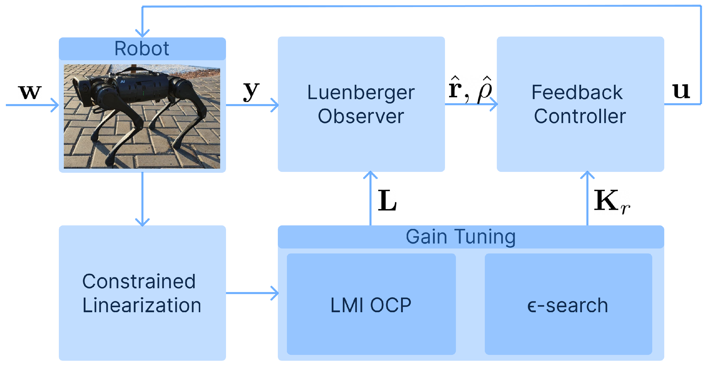
This optimization problem can be efficiently solved using an SDP solver. We will refer to it as the optimal control problem (OCP) in the rest of the paper. It contains $ϵ$ as a parameter. The resulting closed-loop control system is illustrated in the Figure 1.

Remark 2.

The scalar $ϵ>0$ is chosen ahead of solving the problem (57). To overcome the difficulty of choosing the proper ϵ, we use a gridding method, searching over a range of values of ϵ to find the one that provides the best γ. Let $\kappa ={\displaystyle \frac{ϵ}{ϵ+1}}$; hence, $ϵ={\displaystyle \frac{\kappa }{1-\kappa }}$. Since $ϵ>0$, it follows that $0<\kappa <1$. We divide the interval $(0,1)$ evenly, find ϵ associated with each value of κ on that interval, and solve the OCP for that ϵ value. Among multiple OCP solutions, we choose the one that demonstrates the smallest gain γ. This method was introduced in [8].

7. Numerical Simulations and Discussion

To verify the proposed method, we apply it to the design of $H_{\infty }$ control for two mechanical systems: an underactuated three-link robot with a fixed end-effector and a flat quadruped robot model.

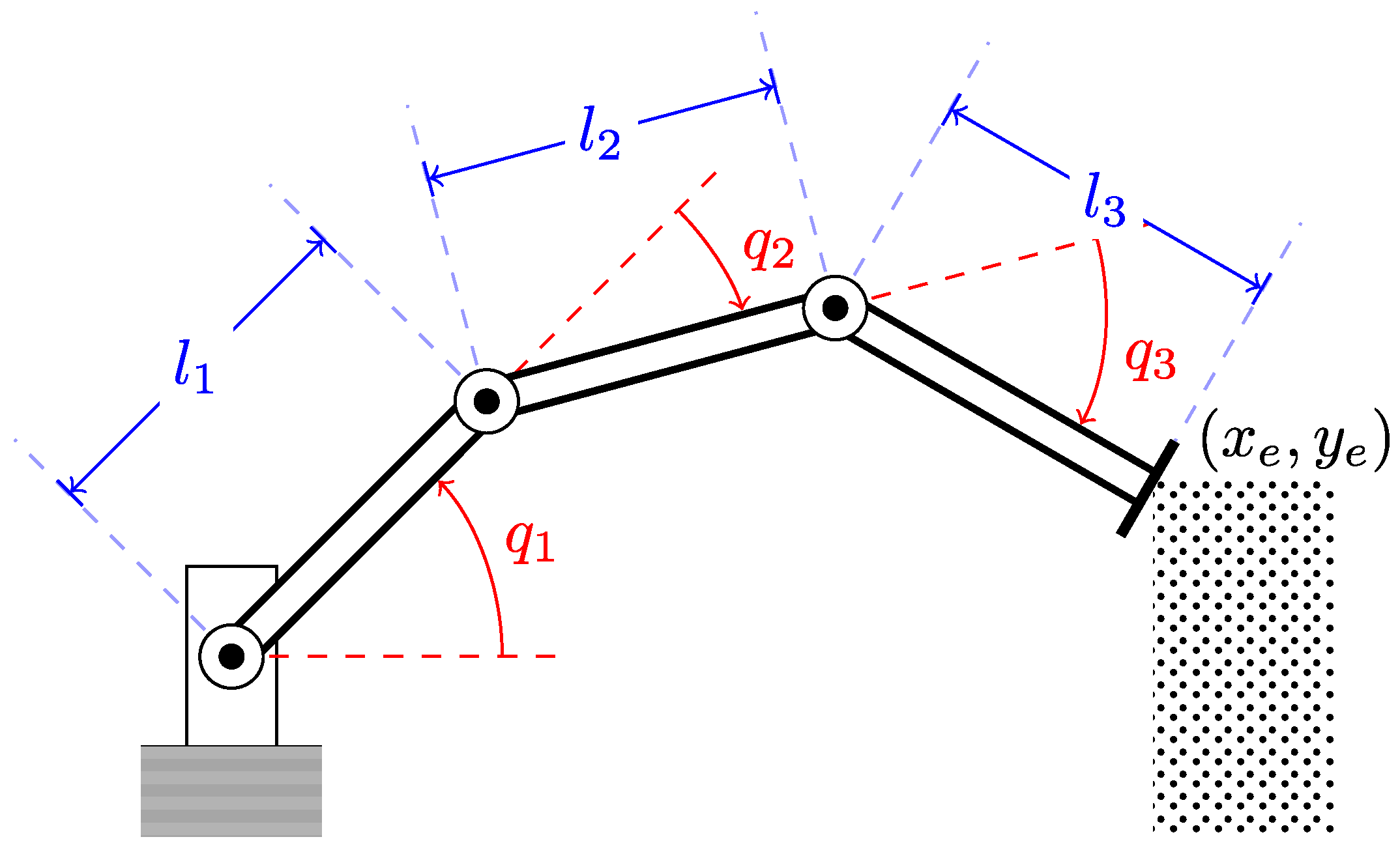
7.1. Constrained Underactuated Three-Link Robot

In this subsection, we design a control law for a serial mechanism consisting of three links connected via rotary joints. Each link has length $l=0.5$ m, mass $m=10$ kg, and inertia 0.2083 kg·m². Let $q_1$, $q_2$, and $q_3$ be joint angles; then, the state of the robot is formed by the joint angles and their derivatives. The end-effector of the robot is fixed, providing two mechanical constraints and leaving the robot with one mechanical degree of freedom, or equivalently, two active states (using terminology proposed in Section 4). A scheme of the robot is shown in Figure 2.

In this experiment, the coordinates at which the end-effector is fixed are $x_e=-0.25$, $y_e=0.79$. The mechanical constraints related to the fixed end-effector have the following form:

$$\left[\begin{array}{c}-lsin\left(q_1\right)-lsin(q_1+q_2)-lsin(q_1+q_2+q_3)\\ lcos\left(q_1\right)+lcos(q_1+q_2)+lcos(q_1+q_2+q_3)\end{array}\right]=\left[\begin{array}{c}{x}_e\\ y_e\end{array}\right].$$

(58)

Choosing the configuration $q_1=\pi /4$, $q_2=-2\pi /3$, and $q_3=0.7\pi$ as the linearization point, we use the method discussed in Section 4 to produce the following linear approximation of the robot model:

$$\left\{\begin{array}{c}\dot{\mathbf{r}}={\mathbf{A}}_r\mathbf{r}+{\mathbf{A}}_{\rho }\rho +\mathbf{B}\mathbf{u}+{\mathbf{D}}_1\mathbf{w},\hfill \\ \mathbf{y}=\mathbf{C}\mathbf{N}\mathbf{r}+\mathbf{C}\mathbf{R}\rho +{\mathbf{D}}_2\mathbf{w},\hfill \\ \mathbf{z}={\mathbf{C}}_1\mathbf{r}+{\mathbf{C}}_2\mathbf{e},\hfill \end{array}\right.$$

(59)

where the state, control, and constraint matrices ${\mathbf{A}}_r$, ${\mathbf{A}}_{\rho }$, $\mathbf{B}$, ${\mathbf{J}}_m$ attain the following values:

$${\mathbf{A}}_r=\left[\begin{array}{cc}0.71& 0.97\\ 1.28& -0.07\end{array}\right],{\mathbf{A}}_{\rho }=\left[\begin{array}{cccc}0.00& 8.56& 0.00& 0.41\\ 0.00& 27.39& 0.00& 1.31\end{array}\right],$$

$$\mathbf{B}=\left[\begin{array}{c}-0.11\\ -0.34\end{array}\right].$$

Matrix $\mathbf{N}$, providing a basis in the null space of the constraint equation, is given as:

$${\mathbf{N}}^T=\left[\begin{array}{cccccc}-0.54& 0.61& 0.50& -0.17& 0.19& 0.16\\ 0.17& -0.19& -0.16& -0.54& 0.61& 0.50\end{array}\right].$$

The external force is assumed to act on the center of mass of the second link in the vertical direction. The corresponding ${\mathbf{D}}_1$ is found to be:

$${\mathbf{D}}_1=\left[\begin{array}{c}0.04\\ 0.13\end{array}\right].$$

We consider the case where the rank of the measurement matrix is 4; additionally, we assume that there is a feed-through from the external disturbance to the measurement. Thus, the measurement matrix $\mathbf{C}$ and the input matrix ${\mathbf{D}}_2$ take the form:

$$\mathbf{C}=\left[\begin{array}{cccccc}1& 0& 0& 0& 0& 0\\ 0& 1& 0& 0& 0& 0\\ 0& 0& 1& 0& 0& 0\\ 0& 0& 0& 1& 1& 0\end{array}\right],{\mathbf{D}}_2=\left[\begin{array}{c}0.01\\ 0.01\\ 0.01\\ 0.01\end{array}\right].$$

The desired output matrices ${\mathbf{C}}_1$ and ${\mathbf{C}}_2$ have the form:

$${\mathbf{C}}_1=\left[\begin{array}{cc}1& 1\end{array}\right],{\mathbf{C}}_2=\left[\begin{array}{cccccc}1& 1& 1& 1& 1& 1\end{array}\right].$$

For brevity, we do not discuss units of the model matrices here; however, we note that the units are chosen in such a way that the input and output signals $w\left(t\right)$, $z\left(t\right)$ are both unitless. We use the static control law (29) to find the following control gain:

$${\mathbf{K}}_{\rho }=\left[\begin{array}{cccc}0.00& 79.32& 0.00& 3.79\end{array}\right].$$

Solving a semidefinite program with the conditions given by (34), minimizing $\gamma$, and choosing the $ϵ$ that gives the lowest value for $\gamma$ using Remark 2, we find the optimal controller and observer gains:

$${\mathbf{K}}_r=\left[\begin{array}{cc}158.25& 154.26\end{array}\right],$$

$$\mathbf{L}=\left[\begin{array}{cccc}-42.97& 11.84& 17.89& 17.59\\ -84.87& 24.29& 36.47& 37.53\\ 3.81& -2.72& -0.88& -0.43\\ -0.37& -4.49& 1.57& 3.31\\ 11.49& -3.91& -3.74& -3.86\\ 1.11& -0.43& 0.84& -1.56\end{array}\right].$$

In our case, the optimal value of $\gamma$ was found to be $0.03$, achieved with $ϵ=0.014$. It was easy to verify that the closed-loop system was stable. We tested the system’s response to signal $w\left(t\right)=\exp (-t)$, whose $L_2$ norm was $0.707$. The ratio between the input and the output signals in that experiment was $0.002$. The time required to solve a single OCP was 0.127 s, while the time for grinding search was 4.967 s with a fixed step of size 0.001 for $\kappa$ over the interval (0,1), as outlined in Remark 2. The gridding is terminated for $ϵ>0.5$ as the solver fails for larger $ϵ$ values.

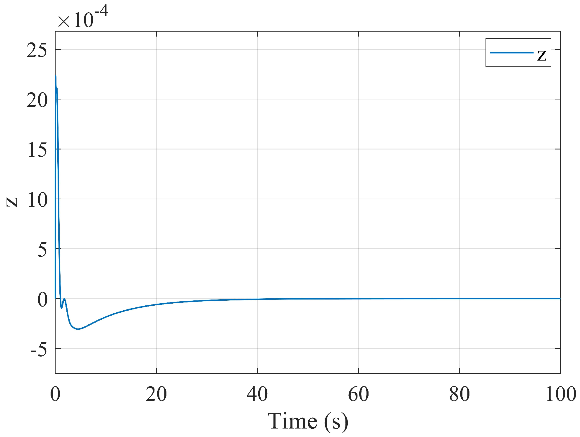
Figure 3 shows the output signal $z\left(t\right)$ for this experiment; Figure 4 shows the same signal plotted together with the input signal $w\left(t\right)$ using logarithmic scale. We observe that the output signal quickly decays to zero. As the input signal vanishes, so does the output. This is the desired behavior of the controller. Let us note that the time horizon of the graph in Figure 3 was chosen with the aim to demonstrate the shape of the signal; however, the primary way of analyzing the signal is linked to its $L_2$ norm, rather than the speed of its decay.

7.2. Flat Quadruped Robot Model

In this subsection, we apply the proposed method to a flat quadruped robot model, as shown in Figure 5. The robot consists of two legs attached to the body via a rotary joint; each leg consists of two links connected via a rotary joint. All joints are actuated, and the feet of the robot remain on the ground throughout the experiment, experiencing constraints associated with unilateral mechanical contact. The lengths of the links are $l_1=0.3$ m, and the length of the body is $l_2=0.5$ m. The mass of each link is 2kg, and the mass of the body is 10 kg. The inertia of each link is 0.0750 kg·m², and the inertia of the body is 0.2083 kg·m². The state of the robot includes the position and orientation of the robot’s body, the robot’s joint angles $q_1,q_2,q_3,q_4$, and the derivatives of all these quantities. We linearize the model around the configuration $q_1=-\pi /6$, $q_2=-\pi /6$, $q_3=\pi /3$, and $q_3=\pi /3$, while the robot’s body is horizontal. The external force is assumed to act on the center of mass of the robot’s body in the horizontal direction.

Performing grid search, we find the optimal $ϵ=0.025$, while the optimal upper estimate of the $H_{\infty }$ gain of the system is $\gamma =0.19$. We test the system with an exponential input $w\left(t\right)=\exp (-t)$, finding that the ratio of $L_2$ norms of the input and the output signals (the latter is chosen as the sum of robot states and observer error states) is $0.04$. The time required to solve a single OCP is 0.507 s, while the total time for gridding search is 28.207 s. The gridding is terminated for $ϵ>0.3$ as the solver fails for larger $ϵ$ values.

Figure 6 shows the output signal $z\left(t\right)$ for this experiment; Figure 7 shows the same signal plotted together with the input signal $w\left(t\right)$ on a logarithmic scale. As we can see, the output signal is orders of magnitude below the input signal; as the input signal vanishes, so does the output. Like in the previous experiment, what we observe is the desired behavior of the controller.

7.3. Limitations

When analyzing the practicality of the proposed method, it is important to consider its computational cost. Computationally expensive control may lead to demanding hardware requirements or a lower-frequency control loop, both of which are undesirable. The proposed $H_{\infty }$ control method presents two sources of computational expense. The first is the linear controller and observer, which are updated on each control loop iteration. They pose a negligible computational expense related to vector addition and matrix–vector multiplication. The second is related to solving OCP (57) multiple times during the gridding, as explained in Remark 2. This is a computationally expensive process: solving the OCP a single time requires 0.127 s for a three-link robot arm and 0.507 s for a quadruped. Gridding pushes these numbers to 4.967 s and 28.207 s, respectively. However, these computations do not need to be performed during the operation of the robot. If the controller and observer gains are tuned before the robot starts its operation, this source of computational expense will not affect the performance of the control system.

The OCP (57) is an SDP problem and thus requires an SDP solver. The computational expense of a semidefinite program grows with the size of its LMI. In the case of problem (57), the size of the LMI (34) grows quadratically (in terms of the number of elements on the LMI matrix) with the increase in the number of state variables describing the robot. Additionally, the SDP solver may fail to solve a large-scale problem even if a solution exists. Other considerations, such as the structure and sparsity of the matrices and the solver settings, also affect the computation time and accuracy [34].

Like other model-based methods, the proposed controller assumes that the system can be modeled by (23) within a reasonable degree of accuracy. This assumption can be violated for several reasons: if the linearization point is too far from the current operational point, if there is significant parametric uncertainty or unmodeled dynamics, if the system undergoes a hybrid transition (e.g., impact or collision), or for other reasons. Given an accurate nonlinear model, it is possible to use nonlinear control tools to ascertain the stability of the nonlinear system controlled by a linear feedback law [35]. Methods such as sum-of-squares programming (SOS) allow us to estimate the region of attraction in the state space where the control law guarantees the stability of the system [36]. Estimating the region where the $H_{\infty }$ norm of the nonlinear system is below a given threshold remains a problem to be solved and poses an interesting direction for further research.

8. Conclusions

In this paper, we presented an $H_{\infty }$ control design method for systems with explicit constraints, taking into account both the geometry of the constraints manifold and the uncertainty in the constraints, which acts as an additive disturbance. We showed a linearization technique, producing a linear model with respect to the active states (the states that lie on the tangent space to the constraint manifold) as well as to the static states (the orthogonal complement to the active ones). We presented an LMI condition required for the desired $H_{\infty }$ gain of the system to be achieved. We demonstrated the work of the proposed method on a constrained underactuated three-link robot as well as on a flat quadruped model. The proposed method is limited by the necessity of finding an accurate linearization for the robot dynamics as well as by the use of semidefinite programming in the formulation of the optimal control problem.