Analysis of Distributed Dynamic Loads Induced by the Own Mass of Manipulator Links and Their Visualization on Interactive 3D Computer Models

Abstract

This study proposes an approach to 3D modeling of spatial manipulators in the Maple 2023 software environment. Algorithms and program codes have been developed to create computer 3D models of manipulators controlled by generalized coordinates. The implementation of these algorithms and program codes has enabled the creation of three-dimensional computer models of manipulators with clear visual representations of links, their cross-sections, kinematic pairs, grippers, and loads, differing in structure and degrees of freedom while ensuring a comprehensive view from all spatial perspectives. During the motion of the manipulator, complex distributed dynamic loads arise in its links due to their intrinsic masses. These dynamic loads create several challenges: for instance, excessive dynamic loads or significant deformation of the links may lead to failure of the manipulator or a loss of precision in the positioning of the gripper. Such loads significantly impact the design, operation, and reliability of manipulators. The study and understanding of dynamic loads in manipulators are crucial areas in mechanics and robotics, enabling the development of more reliable and efficient systems. The Denavit–Hartenberg method was applied to control the motion of the created computer 3D models of manipulators using generalized coordinates. Using the recursive Newton–Euler equations, the necessary kinematic characteristics of the manipulator’s links were determined for calculating the distributed dynamic loads arising from the intrinsic masses of the links at each cross-section, relative to the local coordinate systems rigidly attached to the links. Algorithms and program codes were developed for controlling the motion of 3D models of manipulators, as well as for constructing visual diagrams of distributed dynamic loads in mutually perpendicular planes, formed by the principal axes of the link cross-sections and the axes passing along the longitudinal axes of the links. The implementation of these algorithms and program codes enabled the generation of distribution diagrams of all dynamic loads in all links of the moving manipulator. These diagrams visually illustrate the changes in direction and magnitude of the distributed dynamic loads in all cross-sections of the links throughout the full cycle of the manipulator’s operation. This allows for the consideration of the identified dynamic loads in the strength and stiffness calculations of the manipulator links, which is essential for the design of new innovative manipulators.

1. Introduction

Modern technological advancements have led to increased customer demands for designed products. A high level of competition and diverse operating conditions necessitate the development of products with enhanced characteristics, such as high functionality and quality. In such conditions, engineers must design machines that exhibit flexibility and broad applicability. However, the fabrication of prototypes for all potential devices subject to experimental research is constrained by both economic and time-related factors.

Consequently, modeling becomes a crucial stage in both the design of new structures and the modernization of existing ones. Modern CAD systems not only enable the creation of geometric models but also facilitate kinematic, dynamic, and strength analyses. However, integrating control systems into such applications often presents a complex or even unfeasible challenge. For this reason, Matlab, in combination with the Simulink module, is widely used for modeling control systems.

The study in [1] emphasizes that offline programming (OLP) is an effective method for controlling industrial robots. However, its widespread implementation is hindered by the high cost of commercial OLP systems, which often exceeds the price of the robotic systems themselves. This creates a demand for accessible and efficient OLP solutions based on widely used CAD platforms.

This paper presents the development of the robotic OLP system RobSim, created using SolidWorks Professional 2019 and Microsoft Visual Studio 2010. RobSim is integrated into the SolidWorks environment as an additional tool, providing users with the ability to create, import, and edit objects, as well as conveniently define and modify robot movement trajectories.

In [2], the authors outline the stages of constructing simulation models developed using SolidWorks and Matlab/Simulink. Examples of simulation models include a laboratory hoist and a forestry crane. These models allow for motion visualization, trajectory tracking, and monitoring of velocity and acceleration at any system point.

In [3], a computer model of a three-link vertically walking robot is developed in the Matlab environment, illustrating the basic working principles of such robots. The modeling of the vertical walking robot’s movement was conducted using the SimMechanics library in Simulink within the Matlab environment.

Studies [4,5,6] present a methodology for analytically determining internal forces in the links of planar linkage mechanisms and manipulators, considering distributed dynamic loads arising from the self-weight of the links, for both statically determinate and indeterminate structures. Discrete models were developed, and equilibrium equations were derived to establish the relationship between the force vector and the dynamic characteristics of the links. Additionally, algorithms and software codes were created to generate visual plots of dynamic load distribution, transverse and longitudinal forces, and bending moments, with corresponding results provided.

In works [7,8], it is assumed that the masses are concentrated at the center of gravity of the manipulator links. The inertia forces and the inertia matrix of the i-th link are determined relative to its center of mass. To illustrate the application of the recursive Newton-Euler equations, a two-link manipulator with rotational kinematic pairs is considered.

In the dynamic analysis of a manipulator, gravitational and inertial forces, as well as moments of inertia, are referenced to the center of mass of each link. However, they can be transferred to the axis of rotation of the link using Steiner’s theorem. When analyzing the dynamics of the entire system, forces and moments are referenced to the axes of rotation of each link. Bringing all forces and moments to the rotation axes allows for the formulation of manipulator dynamics in a convenient form (typically a matrix form) that is directly related to actuators.

In [9], a method for modeling the dynamics of manipulators with flexible links is presented. This method decomposes the manipulator into components, with the dynamics of these components determined using Newton–Euler equations and linearized based on state vectors. Transfer matrices are developed to establish the system equations, preventing an increase in the size of the dynamic equations when adding joints or beam elements. The method focuses on computing small-scale dynamic equations of components, simplifying the process.

In work [10], a physically justified approach is presented that accounts for the flexibility of robot links and reducers. The article aims to establish a foundation for modeling flexible robotic structures to enhance accuracy. The elasticity of components is introduced into the discrete-parameter model using pairs of springs and dampers, the number of which is determined by the need to optimize computational costs and simulation time for integrating the model into industrial environments.

In article [11], two novel arm exoskeletons based on pantograph linkages are introduced, capable of supporting loads of up to 9 kg. The pantograph linkage adapts to the arm’s geometry, ensuring support in any position. Gravity compensation is achieved through shoulder support and a counteracting force behind the back. A passive exoskeleton with a gas spring and an active exoskeleton with a motor are described. The forces generated by the gas spring are analyzed and various mechanism configurations are investigated. The equations governing the pantograph linkage are derived, and the exoskeleton forces are modeled with a comparison to measured values.

Article [12] presents a method for analyzing the performance of serial robotic manipulators with gravity balancing under dynamic loads. Torque, power, and energy reduction indices are employed to assess performance in both unbalanced and balanced states. The proposed method enables a comprehensive evaluation of the manipulator while considering dynamic effects. As an example, a three-degree-of-freedom manipulator is examined, in which gravity balancing is achieved using a compact module with a geared spring on each link.

Article [13] introduces an advanced architecture of an internally balanced mechanism based on a four-bar 4R linkage—referred to as the 4R Grand Architecture. The mechanism consists of 24 links and exhibits 26-fold redundant mobility while maintaining mobility with a fixed center of mass. It is demonstrated that all center-of-mass tracking theories for four-bar linkages are contained within this architecture. Additionally, it is shown how new normally constrained two-degree-of-freedom balanced mechanisms can be derived from it by removing specific links.

In article [14], an approach to designing gravity compensators based on planar four-bar linkages and linear springs is presented. A class of compensators comprising 42 types with high efficiency and kinematic simplicity is developed. The compensators are created by combining four-bar linkages with rotating masses and linear springs, whose parameters are optimized to minimize torque within a specified balancing range.

Work [15] investigates the influence of manipulator motion on the base posture of a free-floating space robot. When a target is grasped, a closed system is formed, resulting in more complex dynamic interactions. The interaction is analyzed in both open and closed systems.

In manuscript [16], a mathematical procedure for determining the inertial parameters of maternal manipulators is first described. These parameters are essential for accurate positioning and force control in an electromechanical system designed to assist in surgical operations. The method for determining the mass and center of mass of the manipulator is based on solving static equilibrium equations for rigid bodies. Based on the estimated inertial parameters of the manipulator, the article demonstrates how to determine the force exerted by the manipulator.

Work [17] examines the effect of time-varying inertial loads on the dynamics of parallel manipulators in joint space, particularly during acceleration and deceleration phases. A comprehensive analysis method based on a two-mass model is proposed.

In work [18], with the development of parallel manipulators, the issue of inertia matching has become increasingly significant. However, a clear inertia indicator and a method for its reconciliation have not yet been proposed. This study addresses these aspects using the Stewart manipulator as an example.

Work [19] considers a scenario in which multiple manipulators control a single object. A dynamic model of the system is constructed that explicitly represents the relationship between the object’s dynamics and joint space dynamics, taking into account the object’s dynamics, the dynamics of individual manipulators, and the actuator torques in the joints. Methods are then presented that directly distribute the dynamics of the object and manipulators within the joint space according to criteria based on joint input forces.

In work [20], a computational methodology for determining the maximum payload capacity of a robotic manipulator with joint elasticity is described, considering constraints related to accuracy and actuator characteristics. The maximum payload achievable by the manipulator along a given trajectory is limited by several factors.

One of the key aspects of manipulator design is ensuring the strength and rigidity of its links throughout the entire operational process. The analysis of the stress–strain state of the links is complicated by the fact that the manipulator is in motion, leading to distributed dynamic loads of a complex nature, which are caused by the mass of the links at each of their cross-sections. These loads vary in magnitude and direction depending on the kinematic characteristics of the links.

Since the manipulator is in motion, it is impossible to determine in advance at which cross-section of a link and at what position the maximum internal force or deformation may occur. Therefore, it is necessary to investigate the stress–strain state of the manipulator over the entire operating cycle.

Moreover, it is crucial to visualize the stress–strain state of all links throughout the complete working cycle so that all types of dynamic loads, internal forces, and deformations are clearly visible across all link cross-sections. This allows the designer to analyze the stress–strain state of each link and make well-founded decisions when calculating the strength and rigidity of the manipulator’s links.

Maple is a powerful mathematical software for symbolic and numerical computations, as well as for engineering modeling. It does not require integration with CAD software or other applications to create computer-based 3D models of manipulators controlled by generalized coordinates. In the Maple environment, three-dimensional manipulator models have been developed with clear visual representations of links, their cross-sections, kinematic pairs, grippers, and loads, which vary in structure and degrees of freedom, ensuring a comprehensive spatial view controlled by generalized coordinates. This environment enables the determination of link positions and orientations, the calculation of all kinematic characteristics required for assessing dynamic loads, and their visualization.

The topic of this study is highly relevant and significant in the field of robotics, particularly in the context of manipulator dynamics and design. The study of dynamic loads on manipulators plays a crucial role in the development of more reliable and efficient robotic systems.

2. Materials and Methods

2.1. Algorithm for 3D Modeling of Manipulators in the Maple 2023 Software Environment

The Maple 2023 software environment includes three-dimensional primitives from the plottools package, which enable the construction of 3D shapes and surfaces, such as cones, cylinders, parallelepipeds, and polyhedra. These primitives are used to create links, stands, grippers, and kinematic pairs of manipulators. The generated 3D components in Maple 2023 can be translated along the three spatial axes and rotated around them. Using these links and kinematic pairs, the designer can assemble a 3D model of a manipulator.

Subsequently, all elements of the manipulator are integrated into a single system by introducing fundamental connections (kinematic pairs) from the gripper to the stand. This allows the construction of a complete visual moving model controlled by the generalized coordinates of the manipulator. Maple 2023 provides the capability to connect links both rigidly and while accounting for their relative motion. This feature enables designers to create manipulators with the required structure and specified degrees of freedom. Using the described algorithms in the Maple 2023 environment, program codes were developed for constructing 3D models of manipulators, whose movement is governed by generalized coordinates. The implementation of the developed algorithms and program codes facilitated the creation of three-dimensional computer models of manipulators with distinct representations of links, their cross-sections, kinematic pairs, grippers, and loads, exhibiting various structures and degrees of freedom. All models can be viewed from different angles due to the viewing capabilities of Maple 2023 (Figure 1, Figure 2 and Figure 3). By employing this algorithm, designers can construct computer models of manipulators with any desired structure and varying degrees of freedom. By defining specific patterns of generalized coordinates for the created manipulators, their motion in space can be observed.

To obtain numerical values of the kinematic, dynamic, and strength characteristics of these manipulators, it is necessary to establish Denavit–Hartenberg coordinate systems on their links. When constructing the 3D model of a manipulator in its initial position, the length of the links should be designed relative to the base coordinate system along the same axis as the link lengths in the Denavit–Hartenberg system.

2.2. Position and Orientation of Manipulator Links in Space

In this study, the Denavit–Hartenberg method is used to determine the position and orientation of the manipulator’s links in space. This method was the first to apply 4 × 4 homogeneous transformation matrices to describe the spatial geometry of a manipulator, providing a universal algorithm for deriving its kinematic equations.

A specific choice of coordinate frames for the manipulator’s links allows the transition from one coordinate system to another to be described using only four parameters, rather than six as in the general case. The coordinate system ${\mathrm{O}}_{\mathrm{i}-1}{\mathrm{X}}_{\mathrm{i}-1}{\mathrm{Y}}_{\mathrm{i}-1}{\mathrm{Z}}_{\mathrm{i}-1}$ can be transformed into the system ${\mathrm{O}}_{\mathrm{i}}{\mathrm{X}}_{\mathrm{i}}{\mathrm{Y}}_{\mathrm{i}}{\mathrm{Z}}_{\mathrm{i}}$ through a sequence of one rotation, two translations, and another rotation. The resulting transformation matrix from the coordinate system ${\mathrm{O}}_{\mathrm{i}-1}{\mathrm{X}}_{\mathrm{i}-1}{\mathrm{Y}}_{\mathrm{i}-1}{\mathrm{Z}}_{\mathrm{i}-1}$ to ${\mathrm{O}}_{\mathrm{i}}{\mathrm{X}}_{\mathrm{i}}{\mathrm{Y}}_{\mathrm{i}}{\mathrm{Z}}_{\mathrm{i}}$ is given by the following:

$$A_i^{i-1}=\left[\begin{array}{cccc}{\cos (\theta }_i)& -\sin \left({\theta }_i\right)\cos \left({\alpha }_i\right)& \sin \left({\theta }_i\right)\sin \left({\alpha }_i\right)& a_i{\cos (\theta }_i)\\ \sin \left({\theta }_i\right)& \cos \left({\theta }_i\right)\cos \left({\alpha }_i\right)& -\cos \left({\theta }_i\right)\sin \left({\alpha }_i\right)& a_i{\sin (\theta }_i)\\ 0& \sin \left({\alpha }_i\right)& \cos \left({\alpha }_i\right)& d_i\\ 0& 0& 0& 1\end{array}\right],$$

(1)

where ${\mathsf{\theta }}_{\mathrm{i}}$ is the angle by which the axis $X_{i-1}$ must be rotated around the axis ${\mathrm{Z}}_{\mathrm{i}-1}$ to align with the axis ${\mathrm{X}}_{\mathrm{i}}$. If the kinematic pair $\left(i-1,i\right)$ is rotational, then ${\theta }_i$ is a generalized coordinate; the parameter $d_i$ represents the distance from the origin ${\mathrm{O}}_{\mathrm{i}-1}{\mathrm{X}}_{\mathrm{i}-1}{\mathrm{Y}}_{\mathrm{i}-1}{\mathrm{Z}}_{\mathrm{i}-1}$ of the coordinate system to the intersection of the axis $Z_{i-1}$ with the axis $X_i$, measured along the axis ${\mathrm{Z}}_{\mathrm{i}-1}$. If the kinematic pair $\left(i-1,i\right)$ is translational, then $d_i$ is a generalized coordinate; $a_i$ is the distance between the intersection of the axis ${\mathrm{Z}}_{\mathrm{i}-1}$ with the axis ${\mathrm{X}}_{\mathrm{i}}$ and the origin ${\mathrm{O}}_{\mathrm{i}}{\mathrm{X}}_{\mathrm{i}}{\mathrm{Y}}_{\mathrm{i}}{\mathrm{Z}}_{\mathrm{i}}$ of the coordinate system, measured along the axis ${\mathrm{X}}_{\mathrm{i}}$; ${\alpha }_i$ is the angle of rotation of the axis $Z_{i-1}$ around the axis $X_i$ until it coincides with the axis ${\mathrm{Z}}_{\mathrm{i}}$.

Let us represent the matrix ${\mathrm{A}}_{\mathrm{i}}^{\mathrm{i}-1}$ in the following form:

$$A_i^{i-1}=\left[\begin{array}{cc}{R}_i^{i-1}& {\overrightarrow{O}}_i^{i-1}\\ 0& 1\end{array}\right],$$

(2)

where

$$R_i^{i-1}=\left[\begin{array}{ccc}{\cos (\theta }_i)& -\sin \left({\theta }_i\right)\cos \left({\alpha }_i\right)& \sin \left({\theta }_i\right)\sin \left({\alpha }_i\right)\\ \sin \left({\theta }_i\right)& \cos \left({\theta }_i\right)\cos \left({\alpha }_i\right)& -\cos \left({\theta }_i\right)\sin \left({\alpha }_i\right)\\ 0& \sin \left({\alpha }_i\right)& \cos \left({\alpha }_i\right)\end{array}\right]$$

The matrix ${\mathrm{R}}_{\mathrm{i}}^{\mathrm{i}-1}$ defines the orientation of the axes of the coordinate system ${\mathrm{O}}_{\mathrm{i}}{\mathrm{X}}_{\mathrm{i}}{\mathrm{Y}}_{\mathrm{i}}{\mathrm{Z}}_{\mathrm{i}}$ relative to the coordinate system ${\mathrm{O}}_{\mathrm{i}-1}{\mathrm{X}}_{\mathrm{i}-1}{\mathrm{Y}}_{\mathrm{i}-1}{\mathrm{Z}}_{\mathrm{i}-1}$:

$${\overrightarrow{O}}_i^{i-1}=\left[\begin{array}{c}{a}_i{\cos (\theta }_i)\\ a_i{\sin (\theta }_i)\\ d_i\end{array}\right],$$

(3)

The vector ${\overrightarrow{\mathrm{O}}}_{\mathrm{i}}^{\mathrm{i}-1}$ indicates the position of point $O_i$, which serves as the origin of the coordinate system ${\mathrm{O}}_{\mathrm{i}}{\mathrm{X}}_{\mathrm{i}}{\mathrm{Y}}_{\mathrm{i}}{\mathrm{Z}}_{\mathrm{i}}$, within the coordinate system ${\mathrm{O}}_{\mathrm{i}-1}{\mathrm{X}}_{\mathrm{i}-1}{\mathrm{Y}}_{\mathrm{i}-1}{\mathrm{Z}}_{\mathrm{i}-1}$.

The position and orientation of the $i$-th link of the manipulator relative to the base coordinate system $O_0{X}_0{Y}_0{Z}_0$ are determined by the following expression:

$$A_i^0=A_1^0{A}_2^1{A}_3^2\dots A_i^{i-1}=\left[\begin{array}{cc}{R}_i^0& {\overrightarrow{O}}_i^0\\ 0& 1\end{array}\right].$$

(4)

Using the matrix ${\mathrm{A}}_{\mathrm{i}}^0$, the relationship between the position vectors of a given point in the coordinate systems ${\mathrm{O}}_0{\mathrm{X}}_0{\mathrm{Y}}_0{\mathrm{Z}}_0$ and ${\mathrm{O}}_{\mathrm{i}}{\mathrm{X}}_{\mathrm{i}}{\mathrm{Y}}_{\mathrm{i}}{\mathrm{Z}}_{\mathrm{i}}$ can be established:

$${\overrightarrow{r}}_i^0=A_i^0{\overrightarrow{r}}_i^i,$$

(5)

where ${\overrightarrow{\mathrm{r}}}_{\mathrm{i}}^{\mathrm{i}}=[\begin{array}{ccc}{\mathrm{x}}_{\mathrm{i}}& {\mathrm{y}}_{\mathrm{i}}& \begin{array}{cc}{\mathrm{z}}_{\mathrm{i}}& 1\end{array}\end{array}{]}^{\mathrm{T}}$ is a column matrix that defines the position of any point on the i-th link relative to the coordinate system ${\mathrm{O}}_{\mathrm{i}}{\mathrm{X}}_{\mathrm{i}}{\mathrm{Y}}_{\mathrm{i}}{\mathrm{Z}}_{\mathrm{i}}$, which is rigidly attached to the i-th link; and ${\overrightarrow{\mathrm{r}}}_{\mathrm{i}}^0=[\begin{array}{cccc}{\mathrm{x}}_0& {\mathrm{y}}_0& {\mathrm{z}}_0& 1\end{array}{]}^{\mathrm{T}}$ is a column matrix that defines the position of the same point relative to the base coordinate system ${\mathrm{O}}_0{\mathrm{X}}_0{\mathrm{Y}}_0{\mathrm{Z}}_0$, which is rigidly attached to the base.

2.3. Vectors of Angular Velocities, Linear Velocities, and Accelerations of Manipulator Link Points

The vectors of angular velocities and accelerations of the links, as well as the linear velocities and accelerations of the manipulator link points, are determined relative to the base coordinate system ${\mathrm{O}}_0{\mathrm{X}}_0{\mathrm{Y}}_0{\mathrm{Z}}_0$ and the Denavit–Hartenberg coordinate systems associated with the links ${\mathrm{O}}_{\mathrm{i}}{\mathrm{X}}_{\mathrm{i}}{\mathrm{Y}}_{\mathrm{i}}{\mathrm{Z}}_{\mathrm{i}}$ using Newton–Euler recursive equations. The components of these vectors enable the determination of all types of dynamic loads and the identification of their distribution patterns.

In addition to these vector components, determining the dynamic loads acting at the cross-sections of the links requires knowledge of the linear dimensions of the cross-sections and the specific weight of the link material.

In this study, the angular velocity vector ${\overrightarrow{\omega }}_i$ of the $i$-th link relative to the base coordinate system is represented as follows:

$${\overrightarrow{\omega }}_i=\left\{\begin{array}{c}{\overrightarrow{\omega }}_{i-1}+R_{i-1}^0\times {\overrightarrow{z}}_0\times {\dot{q}}_i,ifthei\text{-}thkinematicpairisrotational,\\ {\overrightarrow{\omega }}_{i-1},ifthei\text{-}thkinematicpairistranslational,\end{array}\right.$$

(6)

where $i$ = 1, 2, …, $n$, ${\overrightarrow{z}}_0=(0,0,1{)}^T$, and $R_{i-1}^0$ is defined by Equation (4).

Then, the angular acceleration ${\overrightarrow{\epsilon }}_i$ of the $i$-th link relative to the base coordinate system is determined by the following expression:

$${\overrightarrow{\epsilon }}_i=\left\{\begin{array}{c}{\overrightarrow{\epsilon }}_i=+R_{i-1}^0\times {\overrightarrow{z}}_0\times {\ddot{q}}_i+{\overrightarrow{\omega }}_{i-1}\times \left(R_{i-1}^0\ast {\overrightarrow{z}}_0\ast {\dot{q}}_i\right),\\ ifthei\text{-}thkinematicpairisrotational,\\ {\overrightarrow{\epsilon }}_{i-1},ifthei\text{-}thkinematicpairistranslational.\end{array}\right.$$

(7)

For the linear velocities and accelerations of the origin of the coordinate system of the i-th link of the manipulator relative to the base coordinate system, the following relations hold:

$${\overrightarrow{v}}_i=\left\{\begin{array}{c}{\overrightarrow{v}}_{i-1}+{\overrightarrow{\omega }}_i\times {\overrightarrow{\rho }}_i^z,ifthei\text{-}thkinematicpairisrotational,\\ {\overrightarrow{v}}_{i-1}+{\overrightarrow{\omega }}_i\times {\overrightarrow{\rho }}_i^z+R_{i-1}^0{\overrightarrow{z}}_0{\dot{q}}_i,\\ ifthei\text{-}thkinematicpairistranslational,\end{array}\right.$$

(8)

where ${\overrightarrow{\rho }}_i^z=R_{i-1}^0\ast {\overrightarrow{O}}_i^{i-1}.$

$${\overrightarrow{a}}_i=\left\{\begin{array}{c}{\overrightarrow{a}}_{i-1}+{\overrightarrow{\omega }}_i\times \left({\overrightarrow{\omega }}_i\times {\overrightarrow{\rho }}_i^z\right)+{\overrightarrow{\epsilon }}_i\times {\overrightarrow{\rho }}_i^z,\\ ifthei\text{-}thkinematicpairisrotational,\\ {\overrightarrow{a}}_{i-1}+{\overrightarrow{\omega }}_i\times \left({\overrightarrow{\omega }}_i\times {\overrightarrow{\rho }}_i^z\right)+2{\overrightarrow{\omega }}_i\times {(R}_{i-1}^0{\overrightarrow{z}}_0{\dot{q}}_i)+{\overrightarrow{\epsilon }}_i\times {\overrightarrow{\rho }}_i^z+R_{i-1}^0{\overrightarrow{z}}_0{\ddot{q}}_i,\\ ifthei\text{-}thkinematicpairistranslational.\end{array}\right.$$

(9)

The linear velocity and acceleration of point ${\overrightarrow{P}}_i^i=[\begin{array}{ccc}{x}_i& y_i& z_i\end{array}{]}^T$ of the $i$-th link relative to the base coordinate system are determined by the following expressions:

$${\overrightarrow{v}}_{iP}={\overrightarrow{\omega }}_i\times {(R}_i^0{\overrightarrow{P}}_i^i)+{\overrightarrow{v}}_i,$$

(10)

$${\overrightarrow{a}}_{iP}={\overrightarrow{a}}_i+{\overrightarrow{\omega }}_i\times \left({\overrightarrow{\omega }}_i\times {(R}_i^0{\overrightarrow{P}}_i^i)\right)+{\overrightarrow{\epsilon }}_i\times {(R}_i^0{\overrightarrow{P}}_i^i).$$

(11)

The angular velocity vector $\overrightarrow{{\mathrm{R}}_0^{\mathrm{i}}{\mathsf{\omega }}_{\mathrm{i}}}$ and the angular acceleration vector $\overrightarrow{{\mathrm{R}}_0^{\mathrm{i}}{\mathsf{\epsilon }}_{\mathrm{i}}}$ of the $i$-th link relative to the coordinate system ${\mathrm{O}}_{\mathrm{i}}{\mathrm{X}}_{\mathrm{i}}{\mathrm{Y}}_{\mathrm{i}}{\mathrm{Z}}_{\mathrm{i}}$, which is rigidly attached to the manipulator’s links, are determined by Equations (12) and (13) given below:

$$\overrightarrow{R_0^i{\omega }_i}=\left\{\begin{array}{c}{R}_0^i\ast \left({\overrightarrow{\omega }}_{i-1}+R_{i-1}^0\ast {\overrightarrow{z}}_0\ast {\dot{q}}_i\right),\\ ifthei\text{-}thkinematicpairisrotational,\\ R_0^i\ast {\overrightarrow{\omega }}_{i-1},ifthei\text{-}thkinematicpairistranslational,\end{array}\right.$$

(12)

where $R_0^i={\left(R_i^0\right)}^{-1},$ and $R_i^0$ is defined by Equation (4).

$$\overrightarrow{R_0^i{\epsilon }_i}=\left\{\begin{array}{c}{R}_0^i\ast ({\overrightarrow{\epsilon }}_{i-1}+R_{i-1}^0\ast {\overrightarrow{z}}_0\ast {\ddot{q}}_i+{\overrightarrow{\omega }}_{i-1}\times \left(R_{i-1}^0\ast {\overrightarrow{z}}_0\ast {\dot{q}}_i\right)),\\ ifthei\text{-}thkinematicpairisrotational,\\ R_0^i\ast {\overrightarrow{\epsilon }}_{i-1},ifthei\text{-}thkinematicpairistranslational.\end{array}\right.$$

(13)

The vectors of linear velocities $\overrightarrow{{\mathrm{R}}_0^{\mathrm{i}}{\mathrm{v}}_{\mathrm{i}}}$ and acceleration $\overrightarrow{{\mathrm{R}}_0^{\mathrm{i}}{\mathrm{a}}_{\mathrm{i}}}$ of point ${\mathrm{O}}_{\mathrm{i}}$, which serves as the origin of the coordinate system ${\mathrm{O}}_{\mathrm{i}}{\mathrm{X}}_{\mathrm{i}}{\mathrm{Y}}_{\mathrm{i}}{\mathrm{Z}}_{\mathrm{i}}$, relative to the coordinate system ${\mathrm{O}}_{\mathrm{i}}{\mathrm{X}}_{\mathrm{i}}{\mathrm{Y}}_{\mathrm{i}}{\mathrm{Z}}_{\mathrm{i}}$, are determined by the following expressions:

$$\overrightarrow{R_0^i{v}_i}=\left\{\begin{array}{c}{R}_0^i\ast \left({\overrightarrow{v}}_{i-1}+{\overrightarrow{\omega }}_i\times {\overrightarrow{\rho }}_i^z\right),ifthei\text{-}thkinematicpairisrotational,\\ {R_0^i\ast (\overrightarrow{v}}_{i-1}+{\overrightarrow{\omega }}_i\times {\overrightarrow{\rho }}_i^z+R_{i-1}^0{\overrightarrow{z}}_0{\dot{q}}_i),\\ ifthei\text{-}thkinematicpairistranslational.\end{array}\right.$$

(14)

$$\overrightarrow{R_0^i{a}_i}=\left\{\begin{array}{c}{R}_0^i\ast {(\overrightarrow{a}}_{i-1}+{\overrightarrow{\omega }}_i\times \left({\overrightarrow{\omega }}_i\times {\overrightarrow{\rho }}_i^z\right)+{\overrightarrow{\epsilon }}_i\times {\overrightarrow{\rho }}_i^z),\\ ifthei\text{-}thkinematicpairisrotational,\\ R_0^i\ast {(\overrightarrow{a}}_{i-1}+{\overrightarrow{\omega }}_i\times \left({\overrightarrow{\omega }}_i\times {\overrightarrow{\rho }}_i^z\right)+2{\overrightarrow{\omega }}_i\times \left(R_{i-1}^0{\overrightarrow{z}}_0{\dot{q}}_i\right)+{\overrightarrow{\epsilon }}_i\times {\overrightarrow{\rho }}_i^z+R_{i-1}^0{\overrightarrow{z}}_0{\ddot{q}}_i),\\ ifthei\text{-}thkinematicpairistranslational.\end{array}\right.$$

(15)

During the motion of the manipulator, the points ${\overrightarrow{P}}_i^i=[\begin{array}{ccc}{x}_i& y_i& z_i\end{array}{]}^T$, which are rigidly attached to the link in the coordinate system ${\mathrm{O}}_{\mathrm{i}}{\mathrm{X}}_{\mathrm{i}}{\mathrm{Y}}_{\mathrm{i}}{\mathrm{Z}}_{\mathrm{i}}$, acquire linear velocities and accelerations relative to this coordinate system. These quantities can be determined using the following equations:

$$R_0^i{\overrightarrow{v}}_{iP}=R_0^i\ast ({\overrightarrow{\omega }}_i\times {(R}_i^0{\overrightarrow{P}}_i^i)+{\overrightarrow{v}}_i),$$

(16)

$$R_0^i{\overrightarrow{a}}_{iP}=R_0^i\ast ({\overrightarrow{a}}_i+{\overrightarrow{\omega }}_i\times \left({\overrightarrow{\omega }}_i\times {(R}_i^0{\overrightarrow{P}}_i^i)\right)+{\overrightarrow{\epsilon }}_i\times {(R}_i^0{\overrightarrow{P}}_i^i)).$$

(17)

2.4. Distributed Dynamic Loads Induced by Link Mass During Manipulator Motion

In this study, it is assumed that the cross-sections of the links remain constant and that the mass is distributed along the link’s axis. Based on this assumption, the patterns of dynamic load distribution along the link’s axis are determined.

For a manipulator with constant link cross-sections, the intensity of gravitational force distribution relative to the base coordinate system at any cross-section of the $i$-th link is given by the following vector (unit of measurement (N/m)):

$$\overrightarrow{f_i}={[\mathrm{0,0},-{\gamma }_i{s}_i]}^T,$$

(18)

where ${\mathsf{\gamma }}_{\mathrm{i}}$ is the specific weight of the material of the $i$-th link (N/m³), and ${\mathrm{s}}_{\mathrm{i}}$ is the cross-sectional area of the $i$-th link (m²).

In the coordinate system ${\mathrm{O}}_{\mathrm{i}}{\mathrm{X}}_{\mathrm{i}}{\mathrm{Y}}_{\mathrm{i}}{\mathrm{Z}}_{\mathrm{i}}$, which is rigidly attached to the $i$-th link, the intensity of the gravitational force distribution is given by the following vector:

$$\overrightarrow{R_0^i{f}_i}=R_0^i\ast \overrightarrow{f_i},$$

(19)

where $R_0^i$ is the matrix that defines the orientation of the axes of the coordinate system ${\mathrm{O}}_0{\mathrm{X}}_0{\mathrm{Y}}_0{\mathrm{Z}}_0$ relative to the coordinate system ${\mathrm{O}}_{\mathrm{i}}{\mathrm{X}}_{\mathrm{i}}{\mathrm{Y}}_{\mathrm{i}}{\mathrm{Z}}_{\mathrm{i}}$.

Due to the accelerations of points located along the link’s axis, inertia forces arise, distributed along the axes of the manipulator’s links. If the link’s cross-section is assumed to be constant, then the mass per unit length of the link (cross-sectional mass or mass distribution intensity along the link’s axis) is given by ${\displaystyle \frac{{\gamma }_i{s}_i}{g}}\left({\displaystyle \frac{\mathrm{N}\ast {\mathrm{s}}^2}{{\mathrm{m}}^2}}\right)$. To determine the intensity of inertia forces arising from the linear accelerations of points along the axes of the coordinate system ${\mathrm{O}}_{\mathrm{i}}{\mathrm{X}}_{\mathrm{i}}{\mathrm{Y}}_{\mathrm{i}}{\mathrm{Z}}_{\mathrm{i}}$, which is rigidly attached to the $i$-th link, we construct the inertia intensity mass matrix, which is expressed as follows:

$${\mathrm{m}}_{\mathrm{i}}=\left(\begin{array}{ccc}{\displaystyle \frac{{\mathsf{\gamma }}_{\mathrm{i}}{\mathrm{s}}_{\mathrm{i}}}{\mathrm{g}}}& 0& 0\\ 0& {\displaystyle \frac{{\mathsf{\gamma }}_{\mathrm{i}}{\mathrm{s}}_{\mathrm{i}}}{\mathrm{g}}}& 0\\ 0& 0& {\displaystyle \frac{{\mathsf{\gamma }}_{\mathrm{i}}{\mathrm{s}}_{\mathrm{i}}}{\mathrm{g}}}\end{array}\right).$$

(20)

Then, the intensity of inertia forces in the cross-sections of the $i$-th link is determined by the following expression (unit of measurement (N/m)):

$${\overrightarrow{q}}_i={-m}_i\ast \overrightarrow{R_0^i{a}_{pi}}.$$

(21)

The vector of the distribution intensity of dynamic loads, arising from the intensity of the distributed self-weights of the link cross-sections and the intensity of the distributed inertia forces due to the linear accelerations of the cross-sections, is determined by the following equation:

$${\overrightarrow{F}}_i=\overrightarrow{R_0^i{f}_i}+{\overrightarrow{q}}_i.$$

(22)

To determine the intensity of the distribution of dynamic torsional moments of inertia, arising due to the self-mass of the links during their rotation about their own axes under the influence of angular velocities and accelerations, we calculate the intensity of the axial moments of inertia in the cross-sections of the link.

Figure 4 shows an image of the link’s cross-section, depicted as a quadrilateral representing a thin plate.

If the axes ${\mathrm{X}}_{\mathrm{i}}$, ${\mathrm{Y}}_{\mathrm{i}}$, and ${\mathrm{Z}}_{\mathrm{i}}$ of the cross-section of the $i$-th link are oriented as shown in Figure 4, then the axial moments of inertia relative to these axes are determined by the following expressions (unit of measurement $(\mathrm{N}\ast {\mathrm{s}}^2)$):

$$I_{xi}={\displaystyle \frac{{\gamma }_i{s}_i{c}_i^2}{12g}}, I_{yi}={\displaystyle \frac{{\gamma }_i{s}_i{h}_i^2}{12g}}, I_{zi}={\displaystyle \frac{{\gamma }_i{s}_i(c_i^2+h_i^2)}{12g}},$$

(23)

where $h_i$, $c_i$ are the dimensions of the cross-section of the $i$-th link, and $s_i=h_i\ast c_i$ is the cross-sectional area of the $i$-th link.

The matrix of the intensity of axial moments of inertia for the cross-section of the $i$-th link is given by the following:

$${\mathrm{I}}_{\mathrm{i}}=\left(\begin{array}{ccc}{\mathrm{I}}_{\mathrm{x}\mathrm{i}}& 0& 0\\ 0& {\mathrm{I}}_{\mathrm{y}\mathrm{i}}& 0\\ 0& 0& {\mathrm{I}}_{\mathrm{z}\mathrm{i}}\end{array}\right).$$

(24)

The intensities of the dynamic torsional inertia moments arising in the cross-sections of the $i$-th link are determined using the following relation (unit of measurement—N):

$${\overrightarrow{M}}_i=-\left(I_i\ast \left(R_0^i\times {\overrightarrow{\epsilon }}_i\right)+\left(R_0^i\ast {\overrightarrow{\omega }}_i\right)\times \left(I_i\ast \left(R_0^i\ast {\overrightarrow{\omega }}_i\right)\right)\right).$$

(25)

Using the presented algorithms, program codes have been developed for constructing visual diagrams of dynamic loads distributed on the manipulator’s links.

3. Determination of Dynamic Loads Arising in the Cross Sections of the RRRRT Manipulator Links and Construction of Their Visual Diagrams

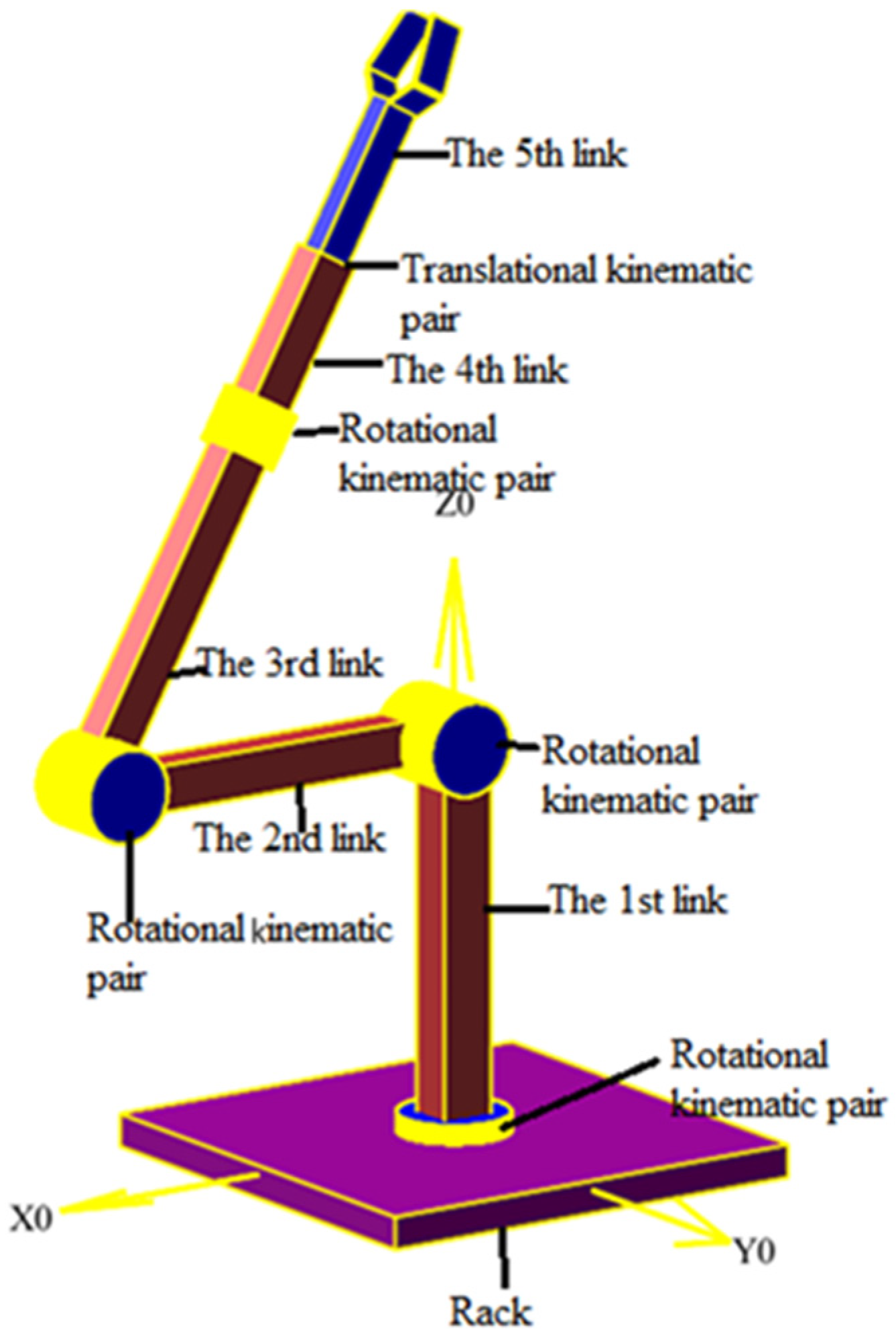
In this study, we examine a 3D model of the RRRRT manipulator (Figure 2), controlled by generalized coordinates. To obtain numerical values for the kinematic and dynamic characteristics of the manipulator’s links, it is necessary to rigidly associate the links with Denavit–Hartenberg coordinate systems. These coordinate systems must be constructed following the rules of the Denavit–Hartenberg method. 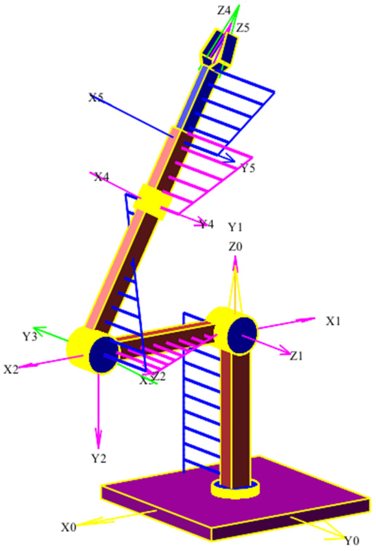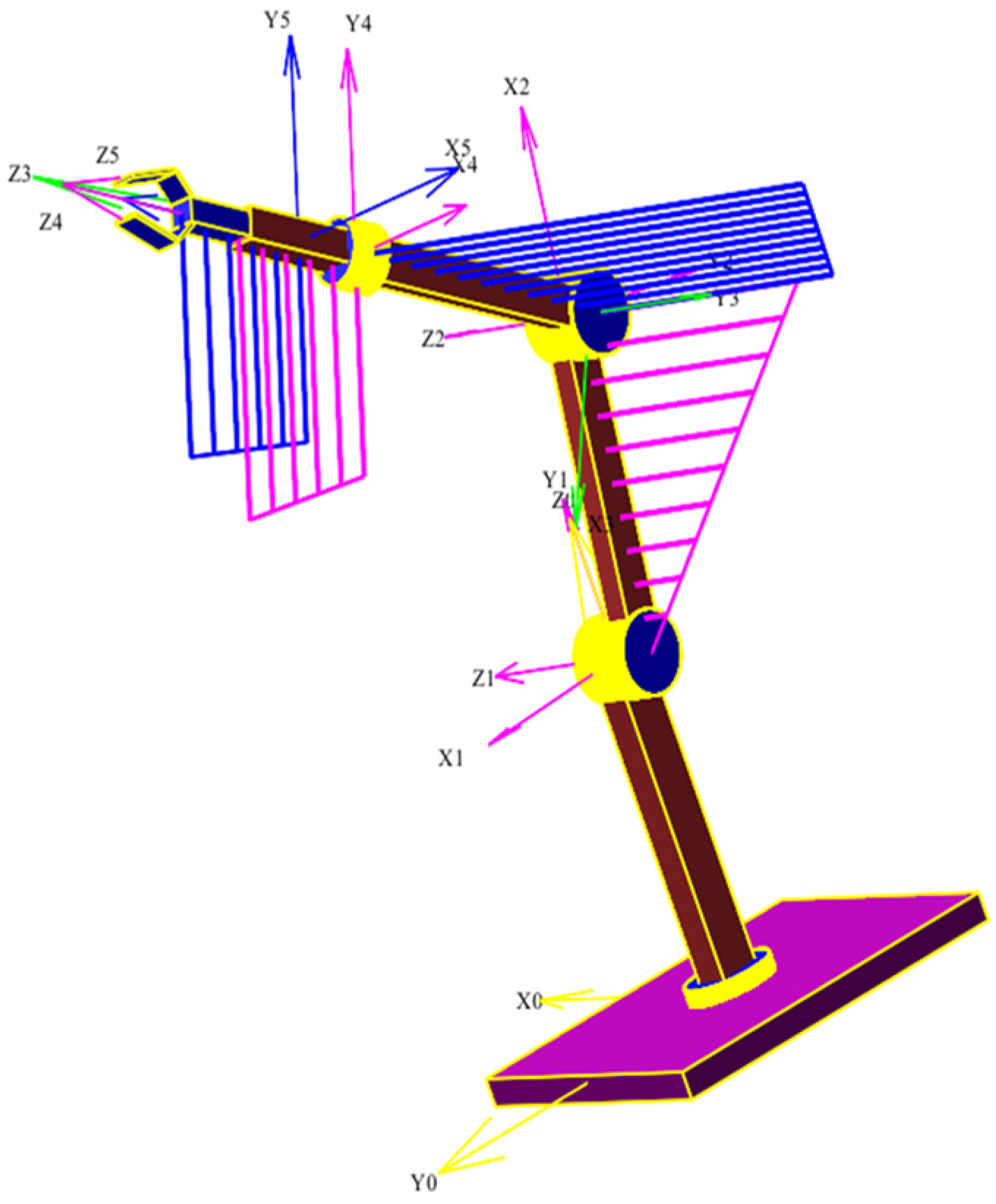Figure 5 illustrates how the links of the considered manipulator are associated with the Denavit–Hartenberg coordinate systems.

After constructing the Denavit–Hartenberg coordinate system for the RRRRT manipulator, the parameters of these coordinate systems can be determined. These parameters are presented in

Table 1. Denavit–Hartenberg coordinate system parameters for the RRRRT manipulator.

Kinematic Pairs	Links Forming Kinematic Pairs	Types of Kinematic Pairs	Values of Coordinate System Parameters
			${\mathsf{\theta }}_{\mathbf{i}}$	${\mathbf{d}}_{\mathbf{i}}$	${\mathbf{a}}_{\mathbf{i}}$	${\mathsf{\alpha }}_{\mathbf{i}}$
1	0, 1	rotational	${\mathsf{\theta }}_1$	$0.85$	$0$	${\displaystyle \frac{\mathsf{\pi }}{2}}$
2	1, 2	rotational	${\mathsf{\theta }}_2$	$-0.09$	$0.8$	0
3	2, 3	rotational	${\mathsf{\theta }}_3$	$-0.09$	$0$	$-{\displaystyle \frac{\mathsf{\pi }}{2}}$
4	3, 4	rotational	${\mathsf{\theta }}_4$	$0.8$	$0$	$0$
5	4, 5	translational	$0$	${\mathrm{d}}_5$	$0$	$0$

.

The generalized coordinate motion laws of the manipulator are defined as follows: ${\theta }_1={\dot{\theta }}_1\ast t$, ${\dot{\theta }}_1=\pi$, ${\ddot{\theta }}_1=0$, where the unit of time is one second, determined by the relation $t={\displaystyle \frac{i}{k}}$, where i = 0…36 represents the discrete positions of the manipulator, and k = 36 is the total number of positions; ${\theta }_2={\dot{\theta }}_2\ast t$, ${\dot{\theta }}_2=\pi$, ${\ddot{\theta }}_2=0$; ${\theta }_3=-{\displaystyle \frac{\pi }{2}}{\ast \dot{\theta }}_3\ast t$, ${\dot{\theta }}_3={\displaystyle \frac{2\pi }{3}}$, ${\ddot{\theta }}_3=0$; ${\theta }_4={\dot{\theta }}_4\ast t$, ${\dot{\theta }}_4=\pi$, ${\ddot{\theta }}_4=0$; $d_5={\dot{d}}_5\ast t$, ${\dot{d}}_5=0.35$, ${\ddot{d}}_5=0$.

The cross-sectional areas of the manipulator’s links (unit of measurement m²) are as follows: $s_1=0.012, s_2=0.008, s_3=0.008, s_4=0.008, s_5=0.0048$.

The specific weights of the materials of the manipulator’s links (unit of measurement N/m³) are as follows: ${\mathsf{\gamma }}_1={\mathsf{\gamma }}_2={\mathsf{\gamma }}_3={\mathsf{\gamma }}_4={\mathsf{\gamma }}_5=78\times {10}^3$.

The cross-sectional dimensions of the manipulator’s links (unit of measurement m) are as follows: ${\mathrm{c}}_1=0.12, {\mathrm{h}}_1=0.1$; ${\mathrm{c}}_2=0.1, {\mathrm{h}}_2=0.08$; ${\mathrm{c}}_3=0.1, {\mathrm{h}}_3=0.08$; ${\mathrm{c}}_4=0.1, {\mathrm{h}}_4=0.08$; ${\mathrm{c}}_5=0.06, {\mathrm{h}}_5=0.04$.

The implementation of the developed algorithms and software enabled the construction of diagrams representing the distribution of dynamic loads across all manipulator links. These diagrams are positioned in mutually perpendicular planes formed by the principal axes of the cross-sections and the longitudinal axes of the manipulator links. The results are presented in Figure 6, Figure 7, Figure 8 and Figure 9.

The diagram of the longitudinal dynamic load distributed along the Y₁ axis of the first link is depicted on the Y₁Z₁ plane and is colored blue. The direction of the distributed longitudinal dynamic loads in the cross-sections, where the ordinates are oriented opposite to the Z₁ axis, is also directed against the Y₁ axis. Conversely, the direction of the distributed longitudinal dynamic forces in the cross-sections, where the ordinates are oriented toward the Z₁ axis, corresponds to the direction of the Y₁ axis.

The diagram of the longitudinal dynamic load distributed along the X₂ axis of the second link is presented on the X₂Z₂ plane in magenta. If the ordinates are directed toward the Z₂ axis, the distributed longitudinal dynamic loads in these cross-sections are aligned with the X₂ axis. Conversely, if the ordinates are directed opposite to the Z₂ axis, the load is oriented in the opposite direction.

The diagram of the longitudinal dynamic load distributed along the Z₃ axis of the third link is drawn in blue on the Y₃Z₃ plane. If the ordinates are directed toward the Y₃ axis, the distributed longitudinal dynamic loads in these cross-sections are aligned with the Z₃ axis. Conversely, if the ordinates are directed in the opposite direction, the loads will be oriented in the opposite direction.

The diagram of the longitudinal dynamic load distributed along the Z₄ axis of the fourth link is presented on the Y₄Z₄ plane in magenta. If the ordinates are directed toward the Y₄ axis, the direction of the distributed longitudinal dynamic loads in these cross-sections will correspond to the Y₄ axis. Conversely, if they are directed in the opposite direction, the loads will be oriented accordingly in the opposite direction.

The diagram of the longitudinal dynamic force distributed along the Z₅ axis of the fifth link is presented on the Y₅Z₅ plane in blue. If the ordinates are directed toward the Y₅ axis, the direction of the distributed longitudinal dynamic loads in these cross-sections will correspond to the Y₅ axis. Conversely, if they are directed in the opposite direction, the loads will be oriented accordingly in the opposite direction.

The diagram of the transverse vertical dynamic load distributed along the X₂ axis of the second link is depicted in magenta on the X₂Y₂ plane. If the ordinates are directed toward the Y₂ axis, the distributed transverse vertical dynamic loads in these sections are also oriented toward the Y₂ axis. Conversely, if the ordinates are directed in the opposite direction, the distributed transverse vertical dynamic loads will be oriented in the direction opposite to the Y₂ axis.

The diagram of the transverse vertical dynamic load distributed along the Z₃ axis of the third link is shown in blue on the Y₃Z₃ plane. If the ordinates are directed toward the Y₃ axis, the distributed transverse vertical loads in these sections are aligned with the Y₃ axis. Conversely, if they are directed in the opposite direction, the distributed transverse vertical dynamic loads will be oriented against the Y₃ axis.

The diagram of the transverse vertical dynamic load distributed along the Z₄ axis of the fourth link is presented in magenta on the Y₄Z₄ plane. If the ordinates are directed toward the Y₄ axis, the distributed transverse vertical dynamic loads in these sections are also aligned with the Y₄ axis. Conversely, if the ordinates are directed in the opposite direction, the distributed transverse vertical dynamic loads will be oriented against the Y₄ axis.

The diagram of the transverse vertical dynamic load distributed along the Z₅ axis of the fifth link is depicted in blue on the Y₅Z₅ plane. If the ordinates are directed toward the Y₅ axis, the distributed transverse vertical dynamic loads in these sections are aligned with the Y₅ axis. Conversely, if they are directed in the opposite direction, the distributed vertical dynamic loads will be oriented against the Y₅ axis.

The diagram of the horizontal dynamic load distributed along the X₂ axis of the second link is presented in magenta on the X₂Z₂ plane. If the constructed ordinates are directed toward the Z₂ axis, the intensity of the horizontally distributed dynamic loads in these sections is also directed toward the Z₂ axis. Conversely, if the ordinates are directed opposite to the Z₂ axis, the intensity of the distributed horizontal dynamic loads is directed against the Z₂ axis.

The diagram of the transverse horizontal dynamic load distributed along the Z₃ axis of the third link is depicted in blue on the Y₃Z₃ plane. The ordinates constructed along the Y₃ axis indicate the magnitude and direction of the intensity of the distributed horizontal dynamic load in these sections. If the ordinates are directed toward the Y₃ axis, the distributed horizontal dynamic loads in these sections are also directed toward the Y₃ axis. Conversely, if the ordinates are directed oppositely, the distributed horizontal dynamic loads in these sections are oriented in the opposite direction from the Y₃ axis.

The diagram of the transverse horizontal dynamic load distributed along the Z₄ axis is represented in magenta on the Y₄Z₄ plane. If the obtained ordinates are directed toward the Y₄ axis, the distributed horizontal dynamic loads in these sections are also directed toward the Y₄ axis. Conversely, if they are directed oppositely, the distributed horizontal dynamic loads in these sections are oriented in the opposite direction toward the Y₄ axis.

The diagram of the transverse horizontal dynamic load distributed along the Z₅ axis is shown in blue on the Y₅Z₅ plane. If the obtained ordinates are directed toward the Y₅ axis, then the distributed horizontal dynamic loads in these sections are also directed toward the Y₅ axis. If they are directed oppositely, then the direction of the horizontal dynamic loads in these sections will be opposite to the direction of the Y₅ axis.

The diagram of the transverse horizontal dynamic load distributed along the Z₅ axis is depicted in blue on the Y₅Z₅ plane. If the obtained ordinates are directed toward the Y₅ axis, the distributed horizontal dynamic loads in these sections are also oriented toward the Y₅ axis. Conversely, if they are directed oppositely, the direction of the horizontal dynamic loads in these sections will be opposite to the Y₅ axis direction.

The distributed torque moments along the second link are represented in the X₂Z₂ plane in magenta. The direction and magnitude of the torque moment in this section are indicated by ordinates aligned along the Z₂ axis. If the ordinate is directed along Z₂, the torque moment in the section induces a counterclockwise rotation about the X₂ axis. Conversely, if the ordinate is oriented in the opposite direction, the section rotates clockwise about the X₂ axis.

The dynamically distributed torque moments on the third link are represented in the Y₃Z₃ plane in blue. If the ordinates are directed toward the Y₃ axis, the distributed moments in these sections induce a clockwise rotation about the Z₃ axis. Conversely, if the ordinates are oriented opposite to the Y₃ axis, the distributed dynamic loads cause a counterclockwise rotation of the section about the Z₃ axis.

The dynamically distributed torque moments on the fourth link are depicted in the Y₄Z₄ plane in magenta. If the ordinates are directed towards the Y₄ axis, the distributed moments in these sections induce a clockwise rotation about the Z₄ axis. Conversely, if the ordinates are oriented in the opposite direction to the Y₄ axis, the distributed dynamic loads cause the section to rotate counterclockwise about the Z₄ axis.

The dynamically distributed torque moments on the fifth link are represented in the Y₅Z₅ plane in blue. If the ordinates are directed towards the Y₅ axis, the distributed moments in these sections induce a clockwise rotation about the Z₅ axis. Conversely, if the ordinates are oriented in the opposite direction to the Y₅ axis, the distributed dynamic loads cause the section to rotate counterclockwise about the Z₅ axis.

4. Verification

The spatial positions and orientations of the links of the RRRRT manipulator can be observed in a visualized 3D computer model created using the developed algorithm and software code in the Maple 2023 environment. Verification is performed by comparing the positions and orientations of these models with extracted numerical values. The kinematic parameters of the manipulator, necessary for determining dynamic loads, were calculated using the recursive Newton–Euler formulas and verified using homogeneous transformation matrices. The diagrams of dynamic loads on the links comply with the distribution laws of the obtained loads.

5. Results and Discussion

Algorithms and software codes were developed and implemented in the Maple 2023 environment to construct three-dimensional computer models of manipulators, providing comprehensive visibility from all perspectives in three-dimensional space. By defining specific patterns of generalized coordinates for the obtained manipulators, their motion in space can be observed.

The Denavit–Hartenberg method was employed to determine the positions and orientations of the links of a five-degree-of-freedom manipulator (RRRRT), which consists of six links connected by one prismatic kinematic and four revolute pairs. The vectors of linear velocities, accelerations, angular velocities, and angular accelerations of the manipulator’s link points were determined relative to the Denavit–Hartenberg coordinate systems attached to the links using recursive Newton–Euler equations. The components of these vectors enabled the determination of all four types of dynamic loads and the identification of their distribution patterns.

Algorithms and software codes were developed for determining the distributed dynamic loads occurring in the cross-sections of the RRRRT manipulator links, as well as for visualizing these loads in the form of diagrams illustrating their distribution within the manipulator links throughout the complete operating cycle. The article does not include the codes for computer 3D modeling of the manipulator, dynamic load determination, or the construction of their diagrams.

6. Summary

This study proposes an approach to 3D modeling of spatial manipulators in the Maple 2023 software environment. Algorithms and program codes have been developed to generate computer-based 3D models of manipulators controlled by generalized coordinates. The implementation of these algorithms and codes has enabled the creation of three-dimensional computer models of manipulators with clear visual representations of links, their cross-sections, kinematic pairs, grippers, and loads, varying in structure and degrees of freedom, while ensuring a comprehensive spatial view from all perspectives.

To control the motion of the created computer-based 3D models of manipulators using generalized coordinates, the Denavit–Hartenberg method was applied. Using Newton–Euler recursive equations, the necessary kinematic characteristics of the manipulator links were determined for calculating distributed dynamic loads arising from the self-weight of the links at each cross-section, relative to local coordinate systems rigidly attached to the links.

Algorithms and program codes have been developed for controlling the motion of the 3D manipulator models, as well as for constructing visual diagrams of distributed dynamic loads in mutually perpendicular planes formed by the principal axes of the link cross-sections and axes passing along the longitudinal axes of the links. The implementation of these algorithms and codes enabled the generation of distribution diagrams for all dynamic loads in all links of the moving manipulator. These diagrams visually represent the variations in direction and magnitude of distributed dynamic loads across all link cross-sections throughout the full operational cycle of the manipulator. This approach allows for the consideration of identified dynamic loads in strength and stiffness calculations of manipulator links, which is crucial for designing new innovative manipulators.