Abstract
In known environments, vehicles plan paths to the target and take precautions to minimize risks. Due to limited dynamics, bounded turning radii, and unfavorable initial conditions, they may be momentarily exposed to threats. In this study, we propose multi-objective real-time optimization based on Dubins paths for multiple vehicles. They synchronize target arrival by reasonably changing speeds and selecting paths of similar lengths. The closer the threats are to the robots and the target, the more path options are available. Risk is reduced in path planning by minimizing the duration of exposure to threats. Vehicles strike a balance between exposure to threats and travel time to targets. We use a probability-based approach to reduce the computation burden and select satisfactory paths such that vehicles synchronize target arrival reasonably far away from threats. The performances of the proposed methods are verified in several simulation examples.
1. Introduction
With advancing technologies and a wide range of applications, multiple-vehicle systems research has attracted more and more attention in recent years. As vehicles move in space, they should avoid threats. Due to their design and limited power, they cannot move freely in space. Path planning is needed to find a safe path to reach the target. Such an approach takes the limited mobility of vehicles into account.
Path smoothness is important [1,2] for vehicles with limited turning radii. For those that need to turn to alter directions, the curvature of paths determines whether they can tightly follow the given paths [3,4,5]. Multiple-wheel vehicles can differentiate wheel speeds, and surface or aerial vehicles can flip rudders or fins such that the turning radii are controlled to follow given paths [6]. However, the above methods have not used curvature for advanced path planning. In this paper, we take a step further and use arcs and lines to represent paths. Vehicles can follow paths as soon as new paths are produced. By adjusting radii in real time, vehicles can obtain optimal paths with the multi-objective cost function.
Path planning is important in providing guidance, and vehicles should reach targets and minimize exposure to threats. Swarm intelligence is useful in handling optimization problems and searching for the global optimum, especially for path planning [7,8]. However, it is computationally demanding to process a large number of particles. This limitation weakens the system’s real-time response. In some applications, lingering or hovering consumes fuel, and data transmission is vulnerable to delay. Multi-drone path planners for multi-target search and connectivity were proposed in [9] with adaptive strategies that re-plan paths upon target detection. A team of resource-constrained robots were used in [10] to collect data and minimize estimation error covariance using informative path planning. The authors transformed the routing-constrained planning problem into a mixed integer program. We use path variations to gather the solution space and propose probability-based searching to find the optimal path that shortens overall path lengths, reduces exposure to threats, and synchronizes arrival at the target.
Vehicles need to avoid threats as they move towards targets. Safety constraints were used with fuzzy reasoning in [11], and techniques were implemented for real-time performance. Mobile obstacle estimation was considered in [12] so that the proposed approaches can tolerate disturbances and faults in modeling. Other existing results were published in similar situations and aim to deal with moving obstacles. This paper uses arcs and lines to link paths. The tangent lines are between discs. To some extent, they are robust against mobile targets and threats. As the paths are simple to calculate, vehicles can achieve real-time performance. Obstacles were regarded as hard constraints [13,14], and other researchers considered probabilistic boundaries [15] that take uncertainty into account. This paper considers threats as soft boundaries, inside which intrusions are allowed and require minimization.
Optimal paths are subject to criteria and changes in circumstances. Quality and fast retrieval of the solution are dependent on the search algorithm. The algorithm designs in [14] assumed convexity in paths and used a gradient of criteria function to guide searching. Some works use inequality for theoretical analysis to determine the convergence rate of searching. Constrained reinforcement learning with topological reachability analysis was studied in [16], achieving reductions in distance costs in automated driving experiments. The efficiency of the proposed approach was analyzed theoretically. Some searching algorithms for path planning are based on graph theory [17,18], and modifications occur for fast response and minimization of energy consumption. Multi-stage/multi-step optimization is useful in combining the strengths of different techniques [13]. A novel approach in motion planning was proposed in [19] for vehicles with curvature constraints by treating integrated resource costs as hard constraints. The probabilistic roadmap was used in pathfinding [20] to reduce the computation burden. In this paper, we integrate steer control and path planning so that multiple vehicles avoid threats and synchronize arrival at the target. We propose algorithms to calculate variations in path sequences and use probability-based searching to find the optimal path, which is usually used to provide real-time performance.
Dubins path planning is usually used for vehicles with limited maneuverability. Dubins path optimization was used in [21] to extend a consensus-based bundle algorithm via a distributed genetic algorithm, and its effectiveness was validated through simulations in dynamic reconnaissance scenarios. Path following was investigated in [22], and Dubins path planning was used to integrate the tasks of navigation, guidance, and control. The target-assignment problem was studied in [21] under a Dubins path; it extended the consensus algorithm to generate feasible flight paths. Improved robustness and efficiency were observed in Monte Carlo simulations. A novel approach in motion planning was proposed in [19] for vehicles with curvature constraints that treated integrated resource costs as hard constraints. The method ensured that the total resource cost along a vehicle’s path stayed within a predefined limit, which was especially valuable in high-risk applications like firefighting. In this paper, we incorporate Dubins paths in the simultaneous arrival problem and use probability-based searching to mitigate risk in the presence of non-trivial threats. We propose a consensus-based control strategy on speed and path lengths in real time for multiple Dubin vehicles, and the performance is robust regardless of initial locations and headings.
Recent advances in multi-agent collaborative path planning have introduced decentralized control strategies, real-time optimization techniques, and learning-based methods to overcome these challenges [18]. For example, Qin et al. [15] and Todorovic et al. [5] demonstrated that distributed consensus algorithms and adaptive optimization frameworks can enhance the coordination of heterogeneous agents, enabling improved synchronization even when facing dynamic obstacles. Similarly, Wu et al. [21] integrated assignment strategies with advanced path planning to better manage both threat avoidance and the synchronization of arrival times among agents. A digital-twin-assisted distributed federated reinforcement training framework was introduced in [23] that maintains high-fidelity mapping, improved vehicle efficiency, and reduced collisions and completion times. A blockchain-based distributed multi-agent reinforcement learning (DMARL) algorithm was proposed in [24] that modeled the system as Markov decision processes to jointly minimize travel time and computation latency, achieving proactive load balancing of both road infrastructures and MEC nodes. Despite these promising developments, several limitations remain. Many state-of-the-art methods incur substantial computational complexity and are sensitive to communication delays, which can compromise real-time threat avoidance and synchronization efficiency—especially in environments with rapidly changing conditions. In contrast, our proposed approach builds upon the classical Dubins framework by incorporating a probability-based real-time optimization strategy. This design adapts turning radii and path selection dynamically to minimize both overall path lengths and exposure to threats while also synchronizing arrival times across vehicles. Importantly, it achieves these objectives with lower computational overhead and improved robustness under limited communication, thereby addressing the key shortcomings of both classical and recent methods.
We consider that vehicles move in space amid threats, represented by Dubins paths. The smaller the turning radii are, the better mobility vehicles would gain and the less likely they would be exposed to threats. However, vehicles sometimes need to enlarge turning radii when moving around large threats. Algorithm design for path planning should not only take threat locations but also radii into account. The proposed approach can strike a balance among multiple objectives. The overall optimization objective is to reach the target simultaneously along the shortest path with minimal risk.
In this paper, we propose path planning for multiple vehicles to reach targets simultaneously. They have bounded heading speeds and lower-bounded turning radii. There are threats in space, and measures are taken to avoid exposure to threats. Vehicles need to move in the space amid the threats and reduce their presence inside the threat discs. The contributions of this paper are summarized as follows:
- Multiple vehicles with limited turning radii are coordinated for the simultaneous arrival task in the face of multiple threats. The proposed algorithms focus on target pursuit and the simultaneous arrival problem. The results can be applied to multiple targets with asynchronous arrival at prescribed times;
- Dubins paths are used as actions and a cost function is proposed to evaluate paths in terms of threat avoidance, minimization of path lengths, and simultaneous arrival;
- Soft boundaries are used to describe threats, and momentary intersections are allowed. Collision avoidance can be achieved by reasonably placing weights in the cost function;
- We use the probability-triggered real-time control strategy to reduce path differences, lower communication frequencies, and achieve real-time performance.
The rest of the paper starts with the problem description and preliminaries. Then, we continue with the path planning and define the cost function to evaluate certain paths. We further define the variations in paths and path sequences. Based on these definitions, we propose probability-based learning for path optimization. We propose speed control to enable simultaneous arrival, supported by a theoretical analysis. The proposed approaches are verified with some numerical examples. See Table 1 for a list of the symbols in this paper.

Table 1.
List of symbols.
2. Problem Description and Preliminaries
In this paper, we investigate path planning for multiple vehicles with threats in space. We assume the occurrence of displacements regarding threats. There is occasional lightweight communication with others, and they make real-time decisions on path planning to reach the target and avoid exposure to threats. The vehicles are assumed to have a limited turning radius, which, for round/aerial vehicles, is usually determined by the steer/rudder angles. The shortest path will be made by joining circular arcs of maximum curvature and straight lines [25]. In this paper, the dynamics are ignored and we consider the turning radius a control input.
2.1. Basic Vehicle–Threat Interaction
At instant k, positions of vehicles are established by positioning and communication in local frames as , , the headings as , , the positions of the threats as , , and the position of the target as . This information is either acquired by sensing, communication, or estimation. We use (1) to describe vehicle i.
where is the turning radius of vehicle i at instant k and is the lower bound of turning radius; , is the heading speed of vehicle i at instant k; is the sampling interval. There are some threats in space, and any vehicle that is less than away from threat j is considered to be exposed to the threat. In this paper, we assume for any , and, thus, vehicles can move along the edge of the threat discs.
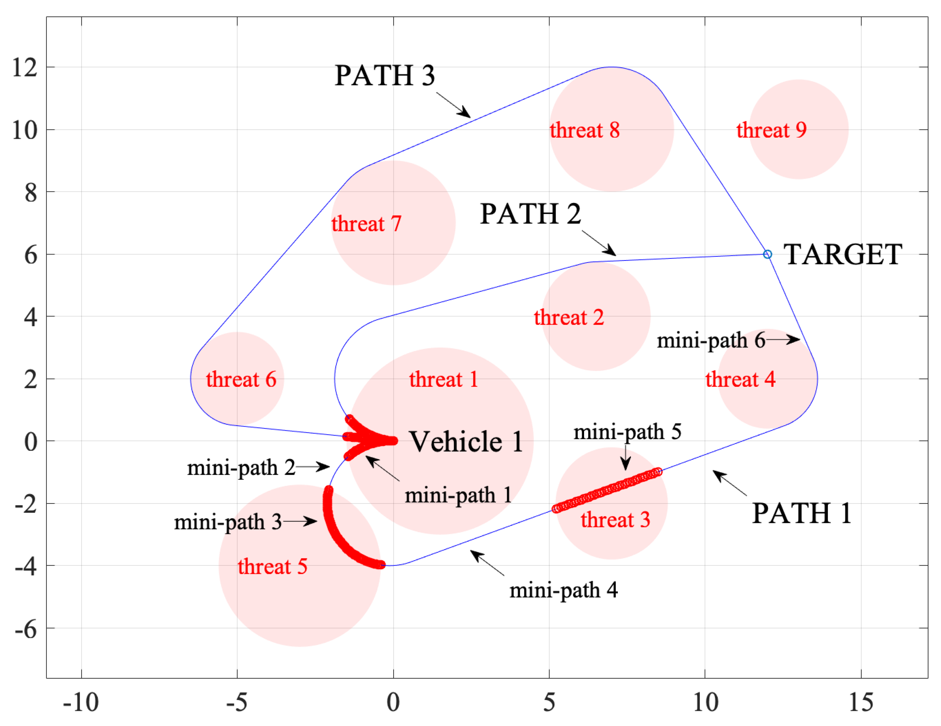
Vehicles have lower-bounded turning radii, and, when they turn left or right, they move along steer circles on their left or right. Take vehicle 1 in Figure 1 as an example. There are two different paths, path 1 and path 2, to reach the target. For path 1, vehicle 1 takes a right turn around the right steer circle to reach the target; along path 2, it takes a left turn around the left steer circle. Given vehicle i, the centers , of the left and right steer circles are given in (2) below, both of whose radii are .
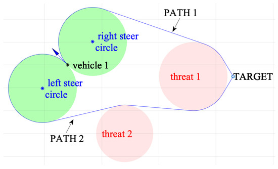
Figure 1.
Vehicle 1 follows paths to reach the target.
Note that If there are no threats, vehicle i turns left or right until it follows a straight line to reach the target. If there are threats, vehicle i takes avoidance action and moves along arcs and tangent lines around and among steer circles and threat discs until it follows a straight line to reach the target.
Between two separated discs, there are four tangent lines; between two intersected discs, there are two tangent lines. A path is defined by the vehicle’s position, heading, turning radius, left/right turn at the start of the path, threats, and the clock/anti-clockwise directions. At instant k, there are a finite total amount of threat discs, steer circles, and targets such that we can use a set in (3) of numbers below to denote a path.
where the path starts by vehicle i moving clockwise, if , or anti-clockwise, if , around right steer circle or left steer circle in (2). Then, vehicle i leaves and moves towards threat along a tangent line such that it moves around threat in clockwise direction, if , or in anti-clockwise direction, if . Vehicle i reaches threats in chronological order in until it arrives at target .
With the positions of threats and the target, vehicles can derive paths to the target. They have access to and can evaluate each other’s paths. As the probabilistic approach is adopted, vehicles plan paths of their own. As a result, the vehicles would update their paths separately and asynchronously. Given the path sequence , we obtain the path in (4) below consisting of some arcs and lines.
where , is an arc on steer circle , and is a tangent line between threat discs and . An arc is defined by the center, radius, start point, end point, and clockwise/anti-clockwise direction at instant k. A tangent line is defined by the start and end points at instant k.
Vehicles can appropriately select paths to reduce overall path lengths or the sum of path lengths inside threats. Take Figure 2 as an example. Given the threat discs in space, vehicle 1 can obtain different paths to reach the target. The picture has three paths, path 1, path 2, and path 3, from vehicle 1 to the target. Along path 1, vehicle 1 takes a left turn and moves around threat 4 to reach the target, and parts of this path lie inside threats 1, 3, and 5. Along paths 2 and 3, vehicle 1 turns right and goes around threats 2 or 6, 7, and 8 to reach the target. In comparison, path 3 has minimal intersection with threats, and path 2 has the shortest overall length with significantly reduced intersection with threats.

Figure 2.
Optional paths from vehicle 1 to the target.
Note that, given and in (3) and (4), and that circles and , or and for any j, are separated, if for any j, then is always valid and not empty. Given that circles and , or and for , are intersected, if there exists such that , then is not valid and empty. Target along the path is considered a circle with a sufficiently small radius whose center is at . If vehicles move or the target changes position, may become empty by .
2.2. Cost Function for Path Planning
After vehicles obtain multiple paths to the target, they select the best one with minimal exposure to threats and shorter overall lengths. Occasionally, parts of the paths lie inside the threat discs. They should be separately calculated. With a lower-bounded turning radius, the path from the vehicle to the target includes linking arcs and lines around and between threat discs. Lengths of paths from vehicles to the target are functions of vehicle positions, headings, and turning radii. For vehicle i at instant k, set of path lengths are calculated and given below.
Path lengths inside threats are considered as function of paths , threat positions and radii at instant k. The set of path lengths inside threats at instant k is given below.
Thus, the overall path length is given in (6) below.
The length sum of paths inside the threat discs is given in (7) below.
Take Figure 2 as an example. In the presence of threats, path 1 can be further divided into 6 mini-paths; those that fall inside the threat discs are drawn as bold lines and arcs in Figure 2, and those that fall outside the threat discs are drawn as light lines and arcs.
The threats in space determine the vehicle paths inside them. The procedure to calculate the lengths is omitted. There are threats in space, resulting in many possible paths to the target. For simultaneous arrival tasks, vehicles select paths with similar overall path lengths. In other words, the goal is to minimize variance given in (8) below.
The suitable paths are found by striking a balance between minimizing overall path length , path variance , and path length sum inside threat discs.
The turning radii of the vehicles are lower-bounded. They can change the radii to achieve better performance if there is a margin with the lower bound. Take Figure 3 as an example. For different turning radii, vehicle 1 can follow different paths to reach the target, and these paths yield different overall path lengths and lengths inside the threat discs. As is shown in the picture, the turning radii for the five paths are , the overall path lengths are 22.3, 27.1, 32.4, 38, and 43.9, and the path lengths inside threats are 10, 9.1, 10.4, 6.1, and 1.5. It can be seen that the path becomes longer as the radius becomes larger and vice versa; the shortest and second shortest path length sum inside threat happens when . Thus, vehicles can reduce exposure to threats by changing turning radii. For simultaneous arrival tasks, vehicles would change radii such that their overall path lengths gradually synchronize.

Figure 3.
Vehicle 1 with different turning radii.
3. Main Methods
3.1. Path Planning and Cost Function
Vehicles’ actions are guided by their paths. We evaluate the cost of action by (9) below.
where are constant coefficients. Vehicles prefer an action obtained by (10) below.
where is a set of path sequences that vehicle i has access to. Such a set can be received from other vehicles, or estimated by recently received path sequences.
Vehicles seek to reach the target with the shortest path length and minimal threat exposure. To reduce the path lengths, we should use larger ; to avoid exposure to threats, we should use larger . For simultaneous arrival tasks, vehicles should eliminate path length differences among them, and, for this purpose, we should enlarge . In cases where threats are scarcely distributed, we should use an significantly larger than and ; for satisfactory performance on simultaneous arrival, should be at least several times larger than .
Vehicles may suffer low communication capacity, and the data transmission is occasionally interrupted in relevance to the size of the data packet. At instant k, is a set of vehicles that vehicle i is communicating with or has communicated with. With communication being considered, we use (11) below for vehicle i to evaluate paths.
where is a set of path sequences of vehicle i and other vehicles that vehicle i received. By (11), vehicles will take an action by (10) below.
The above-mentioned parameters, , and , are important to system performance. They are assumed to be fixed throughout the operations, and it was proven effective in Section 4. A detailed sensitivity analysis is beneficial for future research.
Re-Calculate Path Length Inside Threat Discs
Vehicles make real-time decisions to select the appropriate paths, which are subject to change due to their evolving sub-optimality. The parts of the paths that are closer to the vehicles have a larger influence than those further away, especially for the sake of threat avoidance. By (5), we have . We use below to take this factor into account and re-calculate .
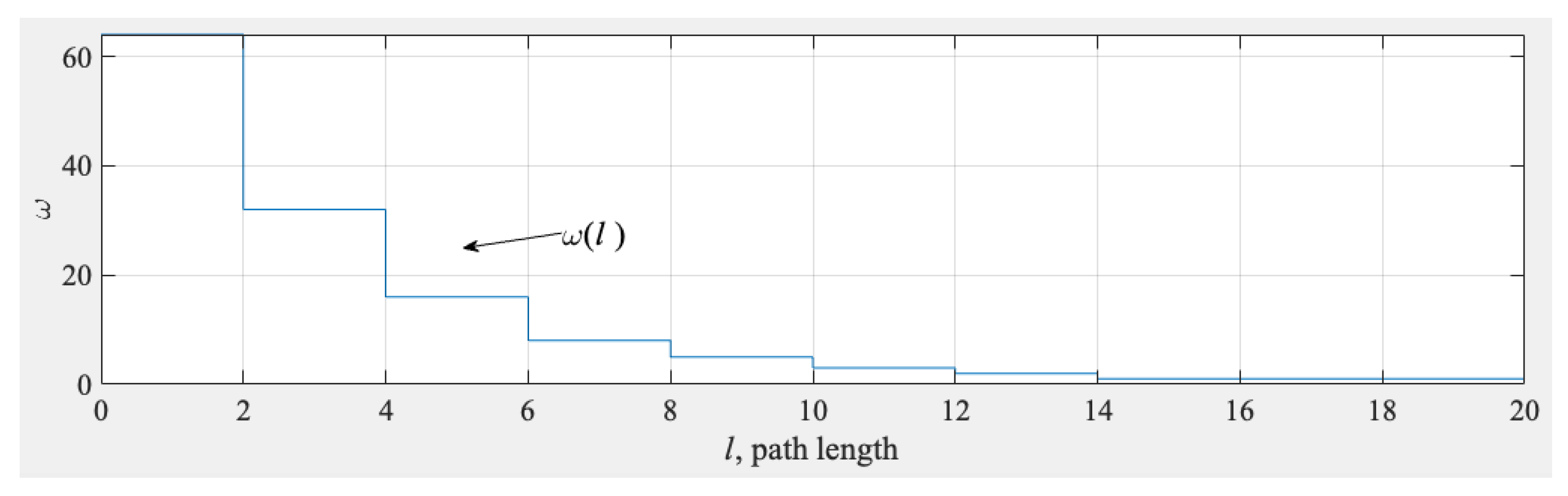
where is path length along from and . has a decreasing value as l increases such that, the further away from vehicle i the path is, the less influential it is on vehicle i. Moreover, the path closer to the vehicle has a larger influence such that it would take more drastic actions to avoid imminent exposure to threats. An example of is given in Figure 4.
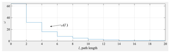
Figure 4.
Curve of .
3.2. Variations in Paths and Path Sequences
In the previous section, we proposed an algorithm of decision-making for selecting the best path. The quality of the solution is determined by , which includes multiple variations in paths or path sequences. By definition in (3), the number of elements in is subject to possible variations induced by positions of vehicles, turning radii, steer circle, threat discs, and the clockwise/anti-clockwise directions that vehicles go around. Specifically, we discuss three types of variations below.
- Type I
- Given , and , we obtain new path sequences by altering members in below.
- Case 1.
- Remove a member in :
- Step 1. Select and remove member .
- Step 2. We have .
- Step 3. We obtain a new path sequence and path .
- Note that cannot be removed because the vehicles are required to reach the target. As vehicle i has a bounded turning radius, cannot be removed. But, it is allowed to alternate between and when alternates between 1 and −1.
- Case 2.
- Insert a member in :
- Step 1. Any threat can be inserted between and , after and before .
- Step 2. We have .
- Step 3. We obtain a new path sequence and path .
- Note that existing threats in shall not be re-inserted as the elements in should be mutually exclusive. Such insertion creates a redundant path that is immediately non-optimal.
- Case 3.
- Shuffle orders of members in :
- Step 1. For , we rearrange their places in .
- Step 2. We have if , or if .
- Step 3. We obtain a new path sequence and path .
- Note that the rearranging can happen once or multiple times to obtain different new path sequences and path . The more the rearranging happens, the more different the new path will be from . Also, the orders of and in should remain unchanged.
- Case 4.
- Reverse clockwise/anti-clockwise directions in :
- Step 1. For members , we have .
- Step 2. We have if or if .
- Step 3. We obtain a new path sequence and path .
- Note that the elements in are either 1 or −1, where 1 represents the clockwise direction and −1 represents the anti-clockwise direction. We obtain a new path sequence by selecting one or multiple elements in , reversing the signs by multiplying by −1 and re-grouping with the other elements in . The more sign reversing happens, the more different the new path will be from .
- Type II
- Given , we obtain new path sequence and path by changing turning radius of vehicle i below:
- Case 5.
- Enlarge ;
- Case 6.
- Reduce ;
where is a constant small value, and it is used to change the turning radius. is used to replace in and we obtain a new path sequence . - Type III
- Given , we obtain new path by changing the starting position:
- Case 7.
- Insert a path in front of that is independent of :
- Step 3. We obtain path sequences and , which are used to obtain and .
- In contrast with the beginning of the path sequence , vehicle i can turn right or left or move straight forward in the next sampling interval. Thus, without changing and and being independent of the path sequence , we insert arcs or line in the first place of path and obtain new paths .
The obtained new paths/path sequences above are included in set , which is used in (10) or (12) to find the best path.
We have presented above the method to generate variable paths for later optimization. Note that our approach intentionally generates vehicle paths with smooth curvature transitions that are constrained to not exceed the vehicles’ maximum turning capacity. In other words, by design, the curvature changes in our planned paths always remain within the controllable range of the vehicles, ensuring full compatibility with their dynamic constraints.
3.3. Probability-Based Learning and Path Optimization
In the previous section, we propose cost functions in (9) and (11) to evaluate the quality of paths for vehicles and propose decision algorithms in (10) and (12) to find the locally optimal path. For vehicle i at instant k, the best path is found in set , which is a variation in paths based on the current path sequence . Three types and seven cases are considered in obtaining variations in or . One or multiple of these cases can be used, and, the more cases are used, the more different the obtained path could potentially be from . Different cases lead to various paths, and the quality of the solution can be improved by selecting preferable cases in search of the best path.
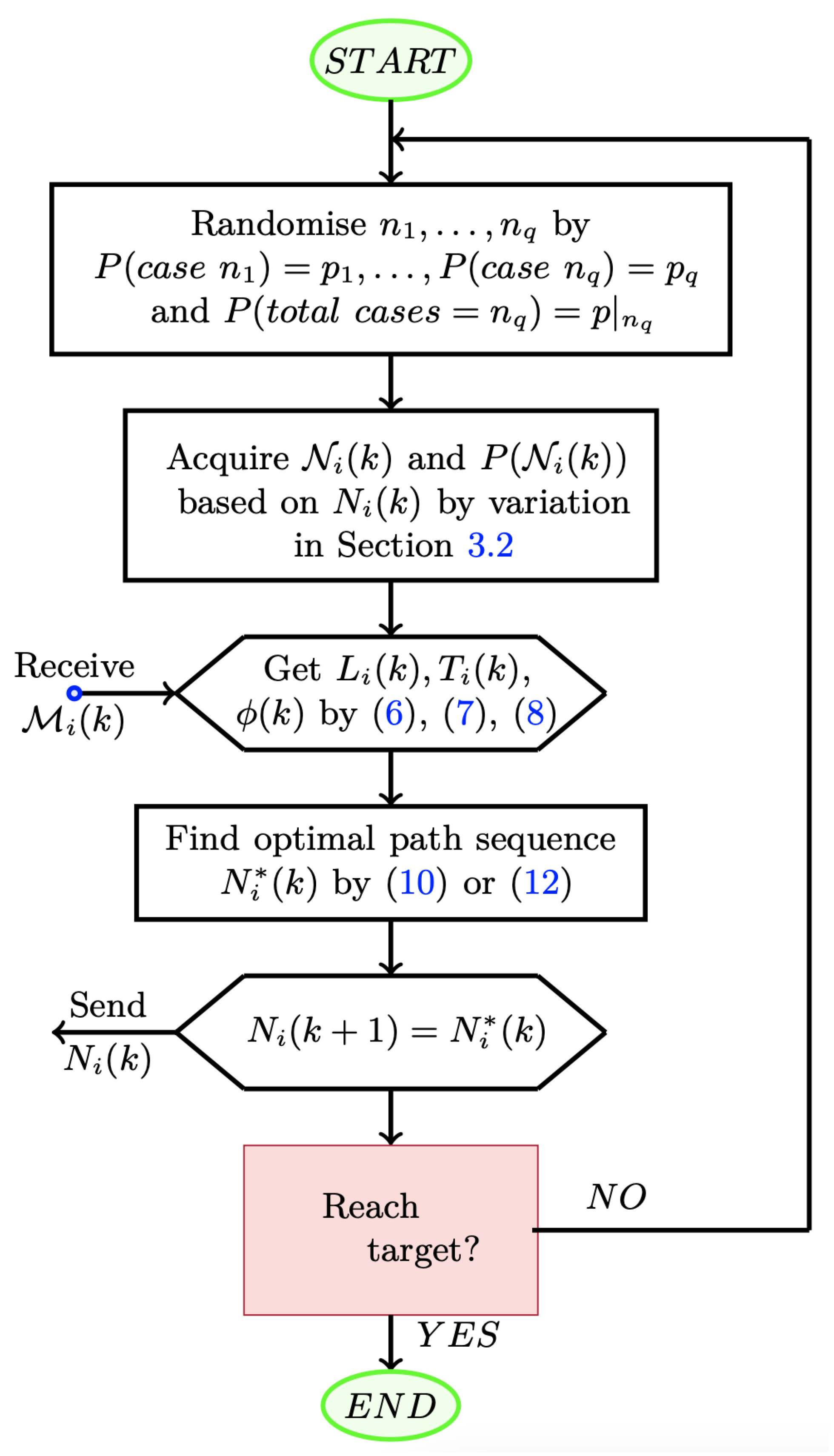
At instant k, we use to represent the possibility that vehicle i uses case j to obtain new path variation, and the possibility of using a total number of cases is . We use the flowchart in Figure 5 to automate the process. At each iteration, an optimal path sequence is found in . Vehicle i will use to update and follow the optimal path until it reaches the target.

Figure 5.
Flowchart for path variation and optimization.
Vehicles are equipped with sensors and receivers to measure the distance and direction of the target and threats and receive the path lengths of others. is a set of vehicles communicating/communicated with vehicle i at instant k. Due to the imperfection of receivers and transmitters and the existence of disturbances in space, is not updated in real time. During intervals between delayed communications, vehicles need to estimate the progress of other vehicles along their paths.
Vehicles communicate with each other, and different cost values by (9) are obtained. It is important to choose vehicles to communicate with reasonably. In simultaneous arrival tasks, vehicles need to synchronize the path lengths. For vehicle i at instant k, it should communicate with those whose path lengths are closer to the mean length of all accessible vehicles. It is reasonable to assume that, the closer the path length of a given vehicle is to the mean lengths, the more likely it will be communicated with.
At instant k and given vehicle i, we use to represent the possibility that vehicle i receives information (path and speed) from vehicle j and to represent the possibility that there is a number of vehicles communicating with vehicle i. We have
is the instant when vehicle i receives information from vehicle j; is updated to include j, .
At instant k, if vehicle i is not receiving path information from vehicles j, , it needs to estimate its current path by routing.
Update Path Sequence by Routing
Assume that, at instant , vehicle i receives path sequences and from vehicle j. At instant k, vehicle i has to estimate the path sequence for vehicle j. Vehicle i considers vehicle j’s speed to be . It has moved at such speed for . For vehicle i, it is possible to assume that vehicle j has proceeded a distance along path sequence .
For vehicle i to obtain path of vehicle j, the distance is removed from and the remaining path is at instant k. It is considered by vehicle i to be the estimate of vehicle j’s current path to the target. For vehicle j, its actual path at instant k is probably different from such estimate by vehicle i because of speed change or variation and optimization of the path.
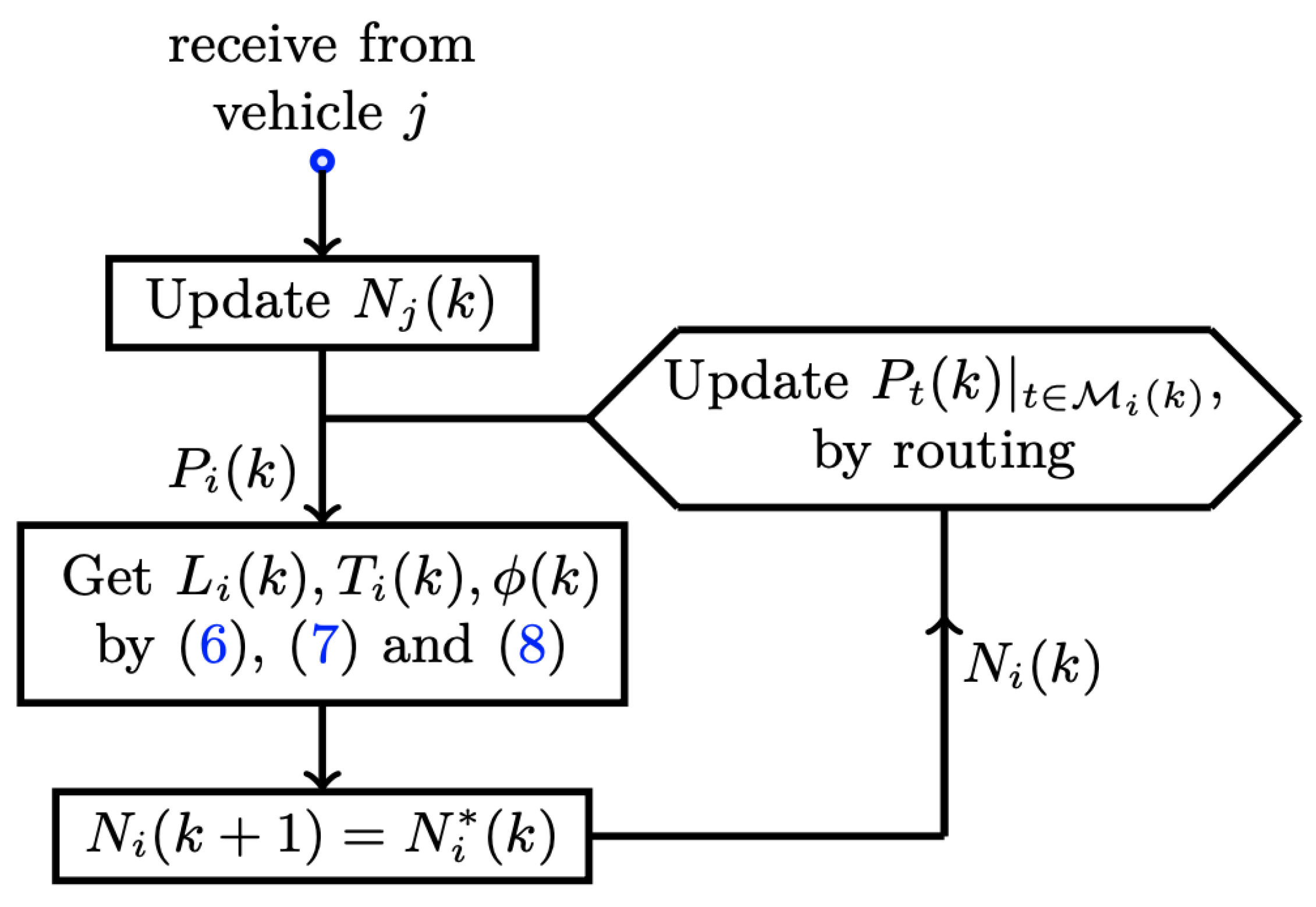
The paths of vehicles belonging to are used by vehicle i to find its optimal path. We use the flowchart in Figure 6 to demonstrate the communication process. Vehicle i can acquire and keep track of path information with occasional communication. As a result of reduced communication frequency, computation burden is reduced and path estimation error is eliminated as soon as unbiased new data arrive. Thus, estimation error would not aggregate if communication were adequately frequent.
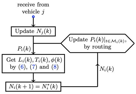
Figure 6.
Flowchart for updating paths by communication and routing.
3.4. Speed Control and Theoretical Analysis
In this paper, we assume that vehicles can alter their speeds. For simultaneous arrival tasks, vehicles use path planning to reduce the differences in their path lengths. For those with shorter path lengths, they should slow down, and, for those with longer paths, they should speed up. By reasonably altering speeds, multiple vehicles can reach the target simultaneously. For vehicle i, the path length dynamics are given in (16) and the controller is given in (17) below.
where, at instant k, is the mean path length and is the speed.
The system is stable if .
Proof.
By (16) and (17), stability and convergence are determined by the value of K, and, below, we analyze the conditions for stability and identify factors prescribing convergence rate.
By (17), we have
It follows that
Assume , and then we have (19).
If , then . If , then . The convergence rate is determined by , and, the larger K is, the faster will reach steady state. □
Stability is the basic requirement of the system. The fastest and slowest speeds are bounded if the average speed is bounded. The vehicles are proceeding towards the target, and it matters how long it takes them to reach consensus on speeds. Ideally, consensus on speeds and path lengths should be reached before the vehicles arrive at the target, which is determined by convergence based on further research. Differences in vehicle dynamics significantly affect their capacity for synchronization. In our study, vehicles use a controller to adjust speeds and path optimization to alter turning radii, the latter of which effectively renders the vehicles heterogeneous.
Vehicles will achieve consensus on vehicle speeds if the system is stable.
Proof.
Assume that we have . As long as the system is stable by , then, by (19), we have for and is unbounded. By definition, we have
As for any i, then we have
As , we have
There are a finite number of vehicles, and n is upper-bounded. We have
For any vehicle i, . As , then we have .
Vehicles always move towards the target. Then, we have for any i. Speeds of vehicles are both upper-bounded and lower-bounded, and the lower bound is larger than . As a result, there exists vehicle such that . Then, we have by and .
There are m vehicles whose speeds are faster than , and vehicle is the slowest among these vehicles. We have
Thus, we have
Therefore, as . The same is true for other vehicles whose speeds are faster than the average. In summary, fast and slow vehicles will reach consensus on speeds, and we have for . □
By (16), the convergence of path lengths is determined by vehicles’ speeds. As ’s convergence rate is determined by , we can expect simultaneous arrival by approaching zero as long as the longest path length descends adequately quickly and the shortest path length descends sufficiently slowly. Since the lower and upper bounds of vehicles’ speeds exist, simultaneous arrival may not always happen. Sufficient convergence conditions for speed control are difficult to obtain. The convergence is directly impacted by the overall path lengths of all the vehicles, a product of the multi-robot path optimization process. Such a process is significantly uncertain due to asynchronous optimization parameters, communication constraints, and uncertain locations of risks in the environment. This issue is open to future research.
4. Numerical Examples
In this section, we use some simulations to test the performance of the proposed approaches. The experiments were conducted on a Mac mini 2023 with a multi-core processor, although our implementation was restricted to single-core processing using MATLAB 2023a. The vehicles have limited turning radii, and, at instant k, we have for any . At instant 0, is given below.
where , , , …, in order. The initial positions of vehicles are given below.
where , , …, in order. The initial headings of the vehicles are given below.
where , , …, in order. The positions of the threats and the threat radii are given below.
where , , …, in order and , , …, in order. The position of the target is .
The sampling interval is , and, for cost function, we have , and . Note that we have used a 0.1 s sampling interval to demonstrate the real-time performances. Shorter intervals and more frequent updates would help to synchronize speeds and paths in a shorter time. On the other hand, longer sampling intervals would lead to less frequent updates and failure in simultaneous arrival. This issue is omitted in this study and will be open to future research.
We use to recalculate the path lengths inside threats, and the curve is given in Figure 4. It can be seen that the curve starts high at , and this helps vehicles prone to threat avoidance actions when they are imminent. The curve descends fast as l increases, and this helps vehicles underplay threats far away as they pose fewer risks. Note that the simulations in this section are run on a MacBook Pro 2014 Mid model. When the graphical output is disabled, it typically takes 30 ms or less than 0.1 s to complete the computation in each iteration.
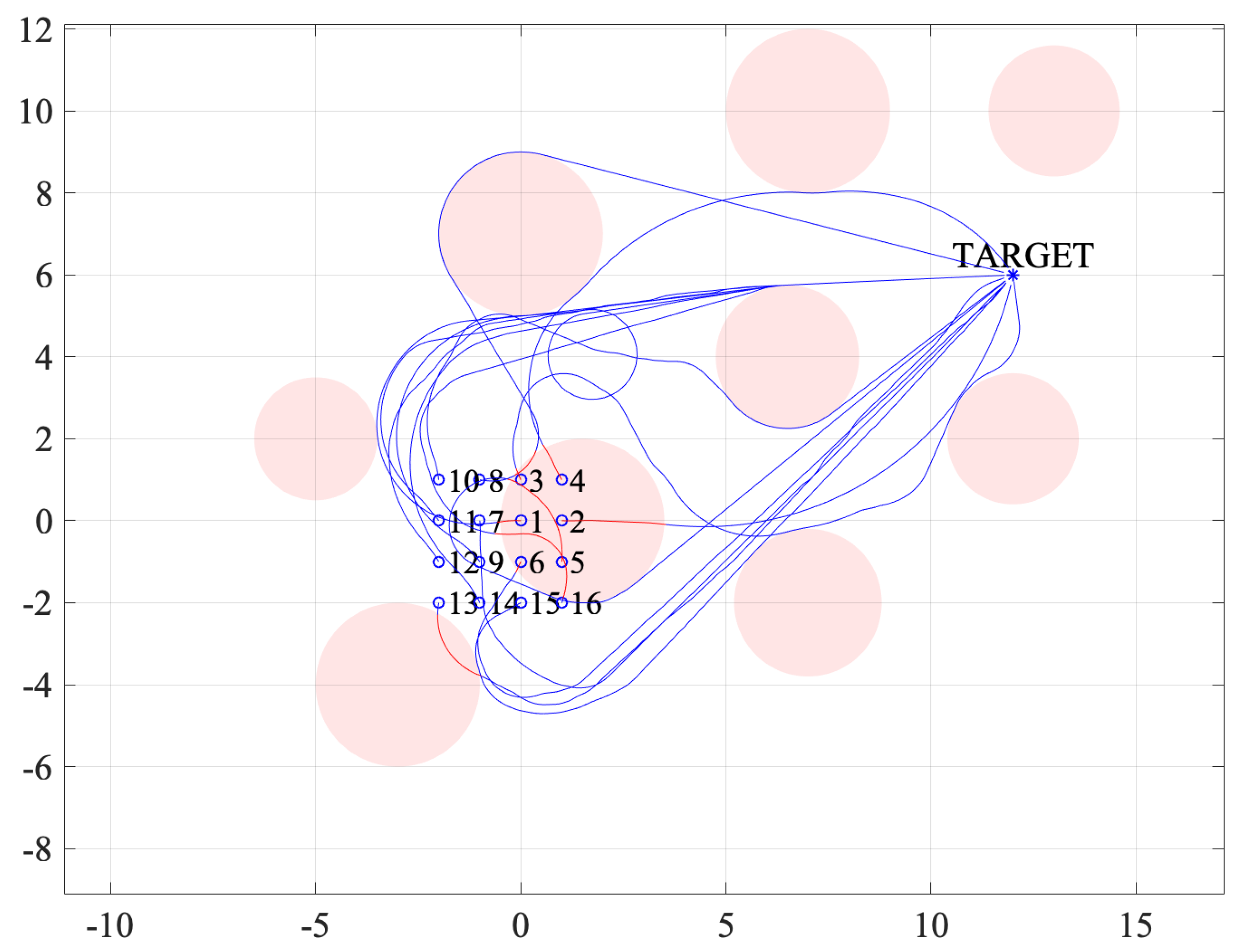
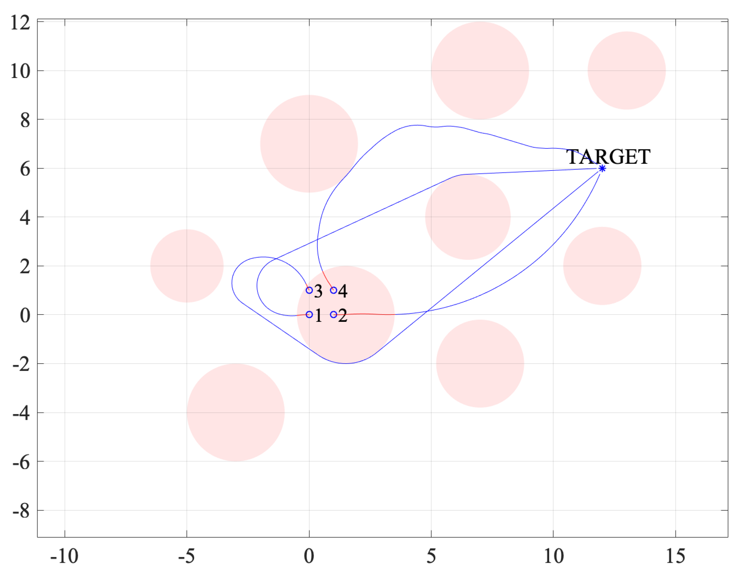
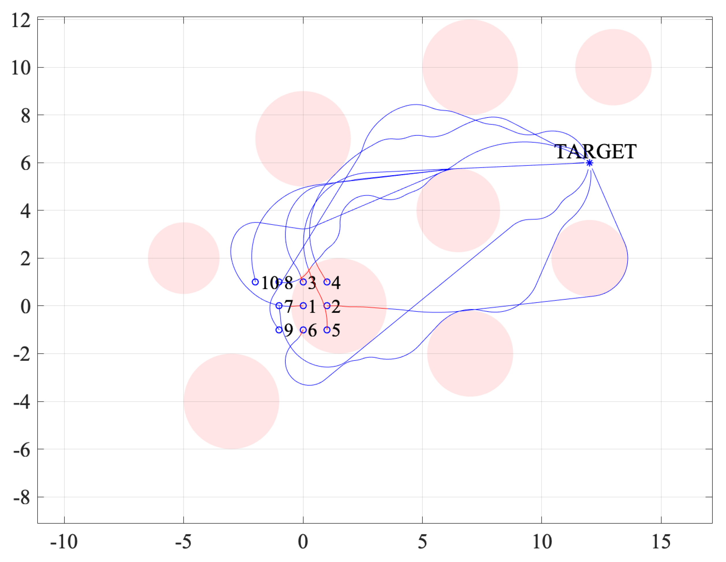
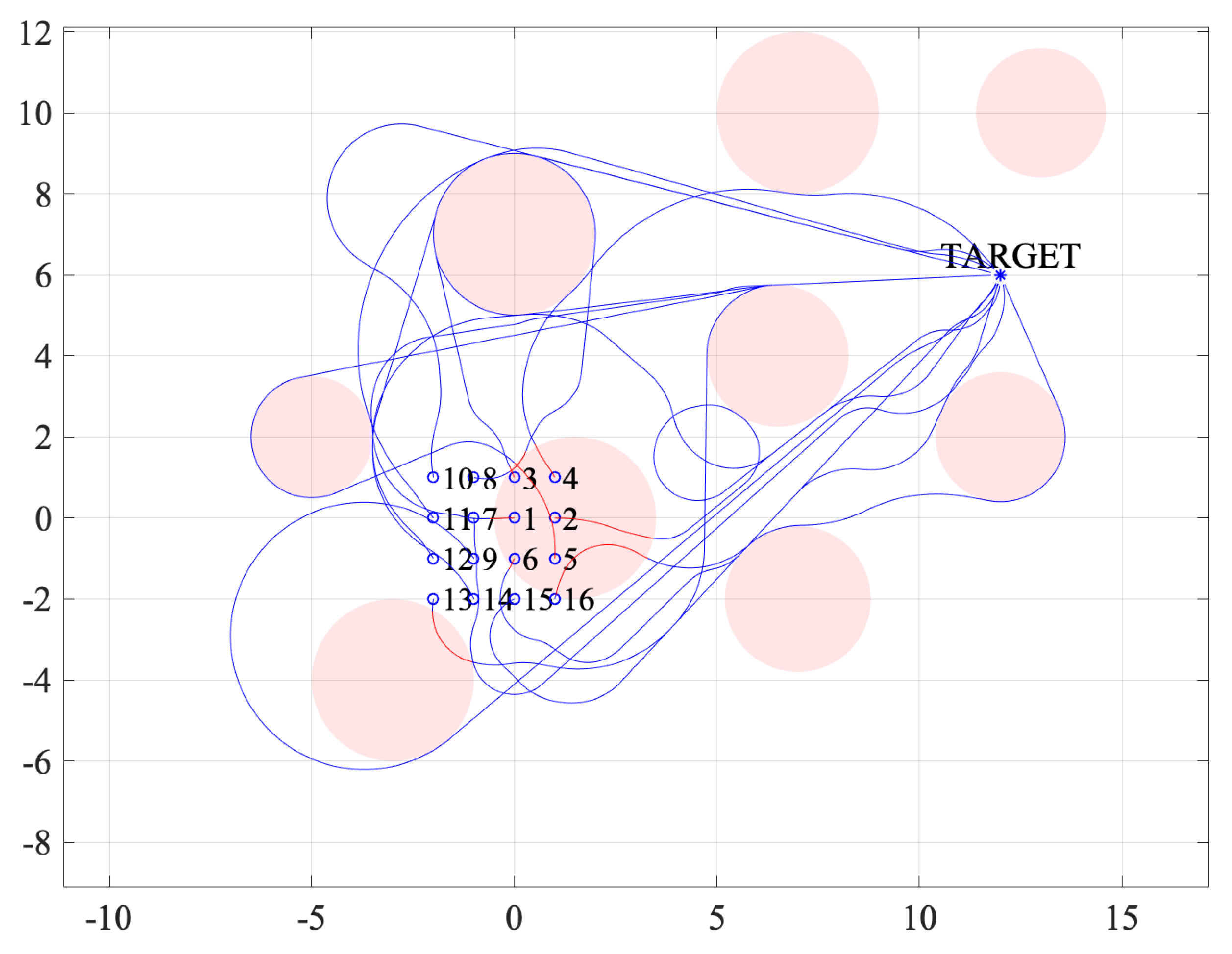
The paths are given in Figure 7, Figure 8 and Figure 9, where there are no communication constraints, and Figure 10, Figure 11 and Figure 12, where there are communication constraints. The threats are shaded, and the target is labeled in the figures. The initial positions of vehicles 1, 2, …, 6 are inside threat discs and those of vehicles 7, 8, …, 16 are outside threat discs. We infer the initial headings of vehicles from the tangent arrows at the initial positions of the vehicles. The vehicles reasonably avoid threats, and they eventually reach the target. The paths are smooth in general. There are few differences between paths under different settings for communication constraints.
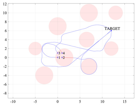
Figure 7.
Paths of 4 vehicles without communication constraints.
Figure 8.
Paths of 10 vehicles without communication constraints.

Figure 9.
Paths of 16 vehicles without communication constraints.
Figure 10.
Paths of 4 vehicles with communication constraints.
Figure 11.
Paths of 10 vehicles with communication constraints.
Figure 12.
Paths of 16 vehicles with communication constraints.
Groups of 4, 10, and 16 vehicles are free to communicate in tasks for simultaneous arrival at the target. The initial positions are , , and , the initial headings are , , and , and the turning radii are , , and . The simulations are divided into two settings, one of which involves communication constraints, the other having none. If there are no communication constraints, every vehicle can communicate with all the rest of the vehicles every . If there are such constraints, vehicles communicate with one of the other vehicles every .
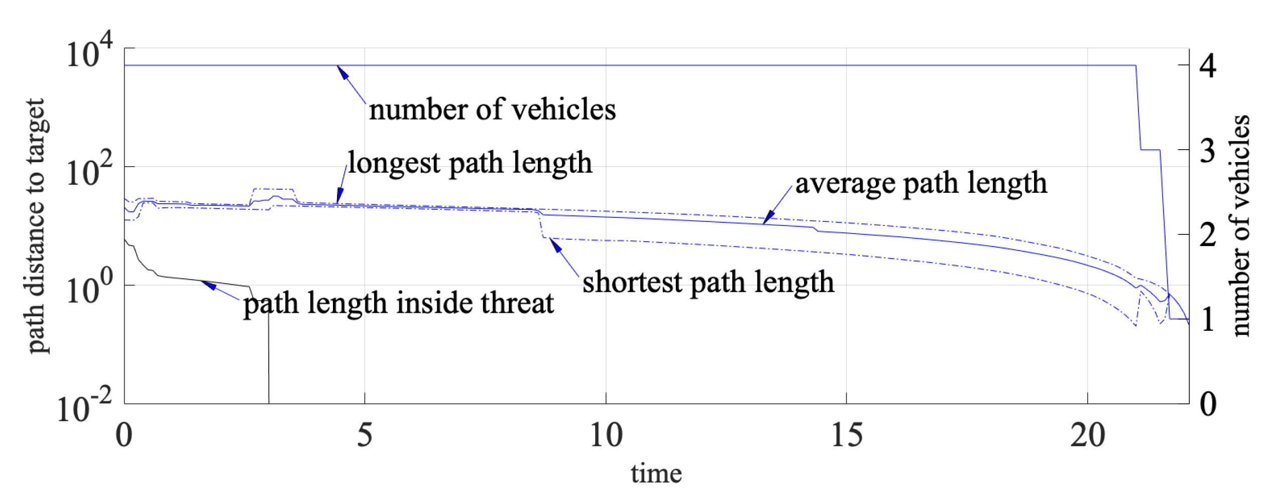
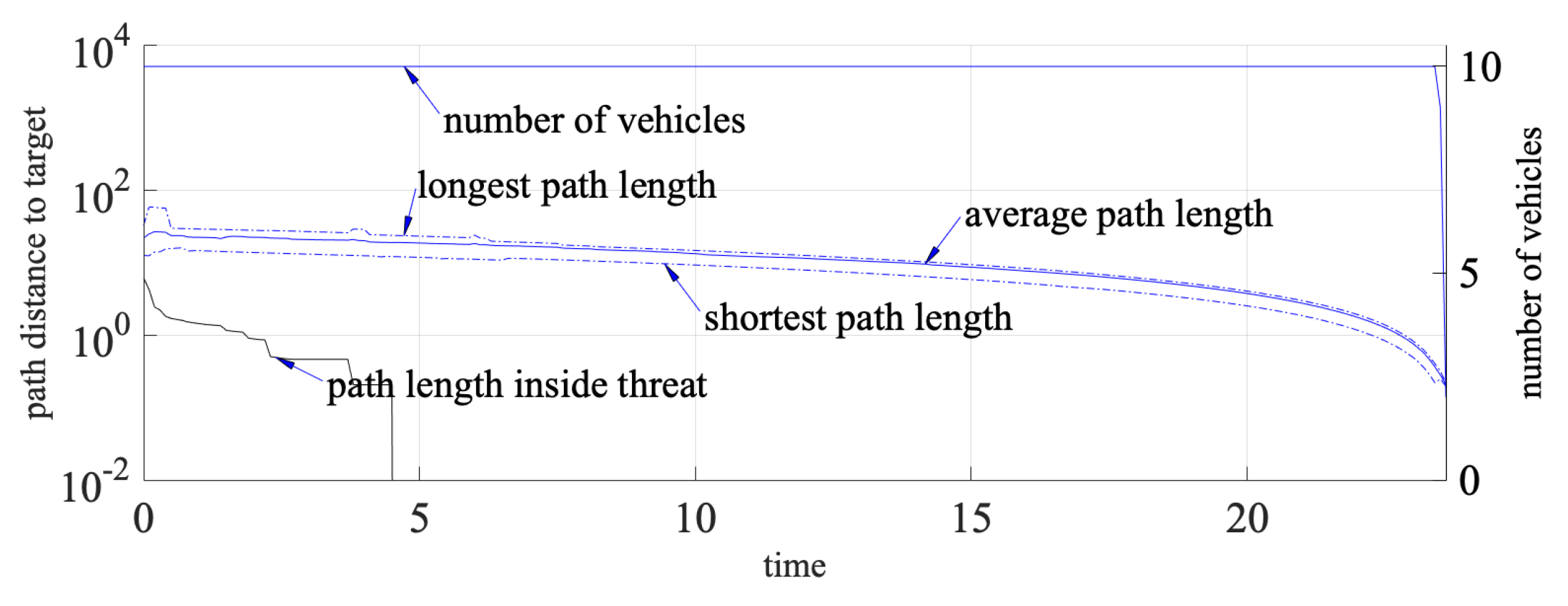
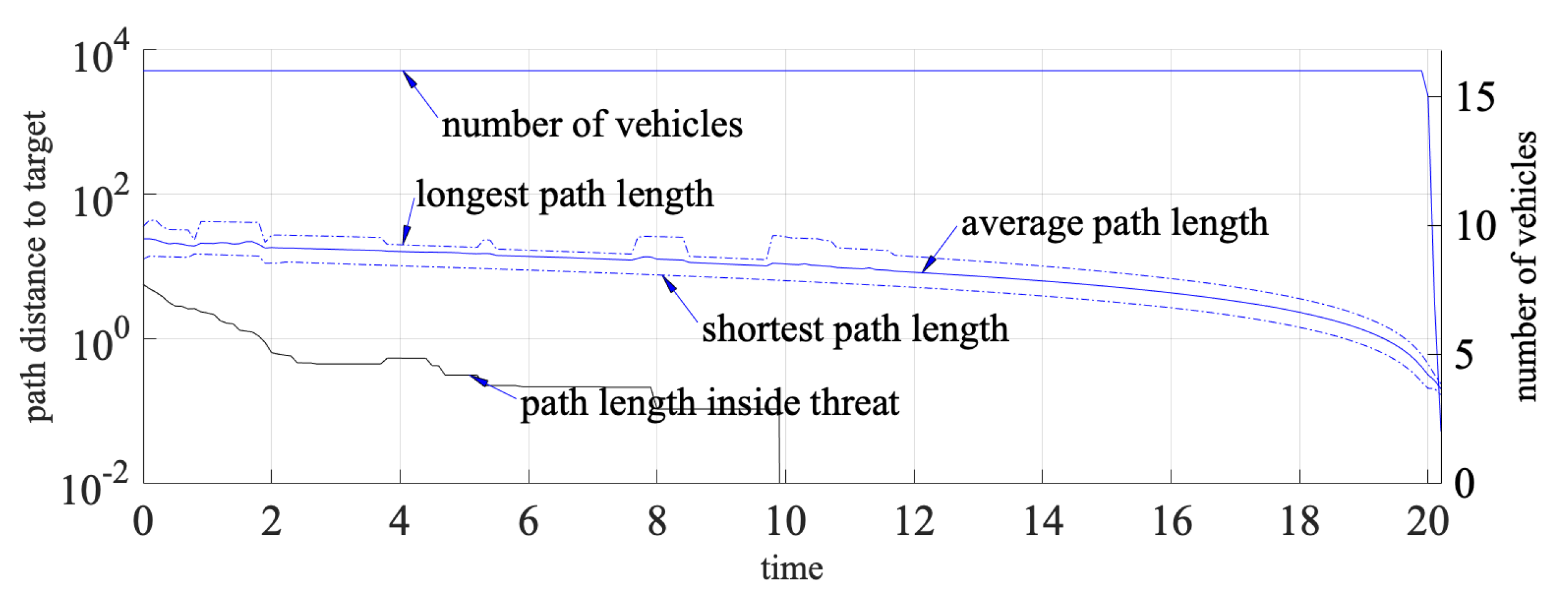
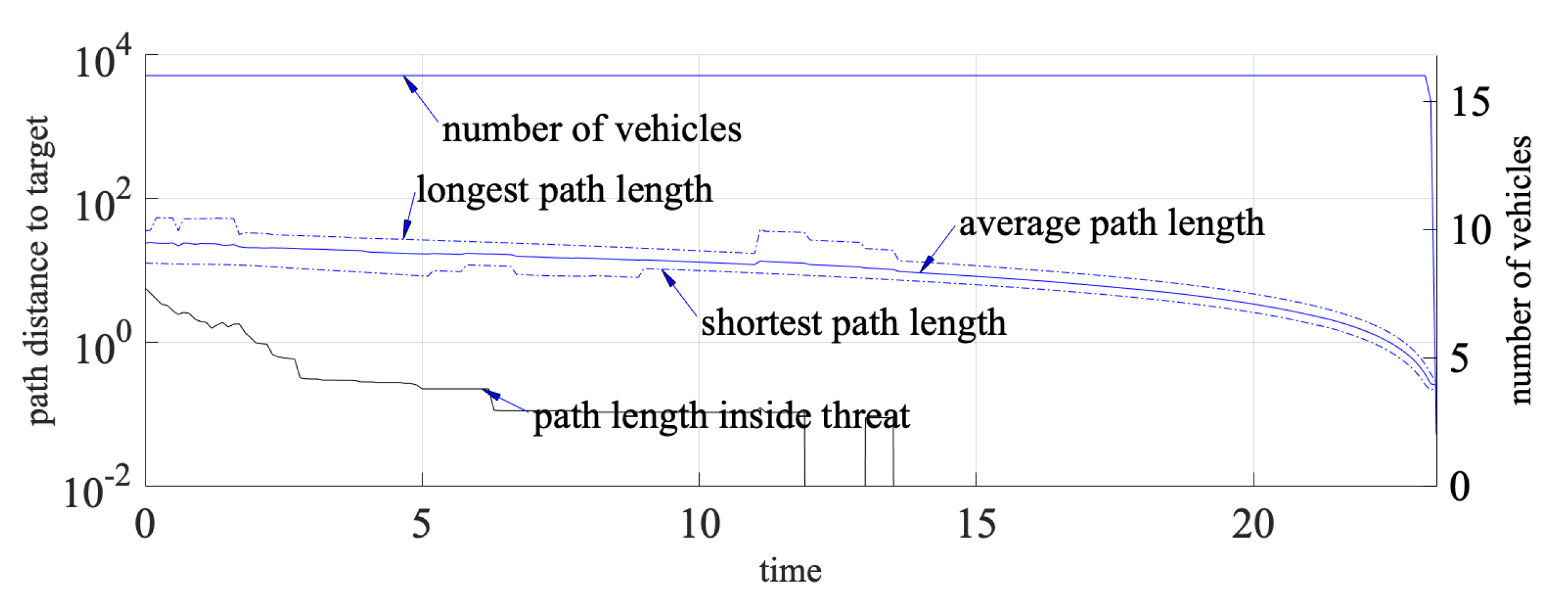
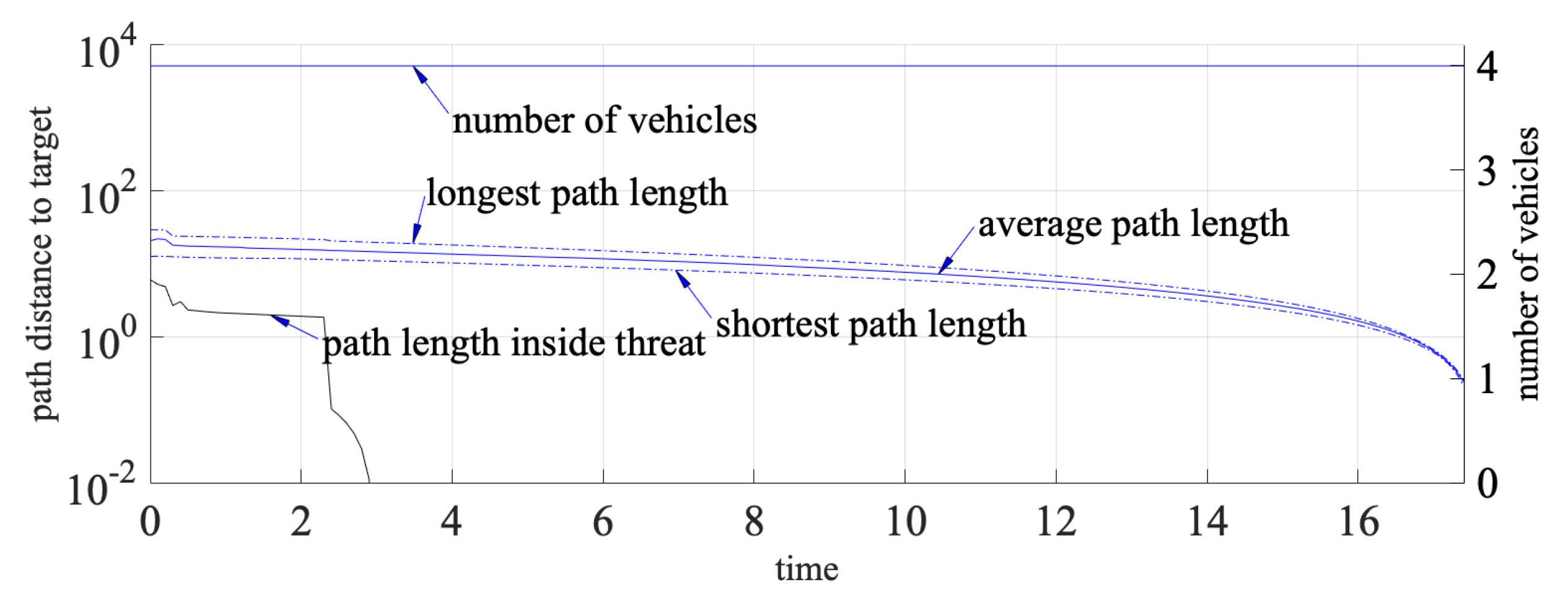
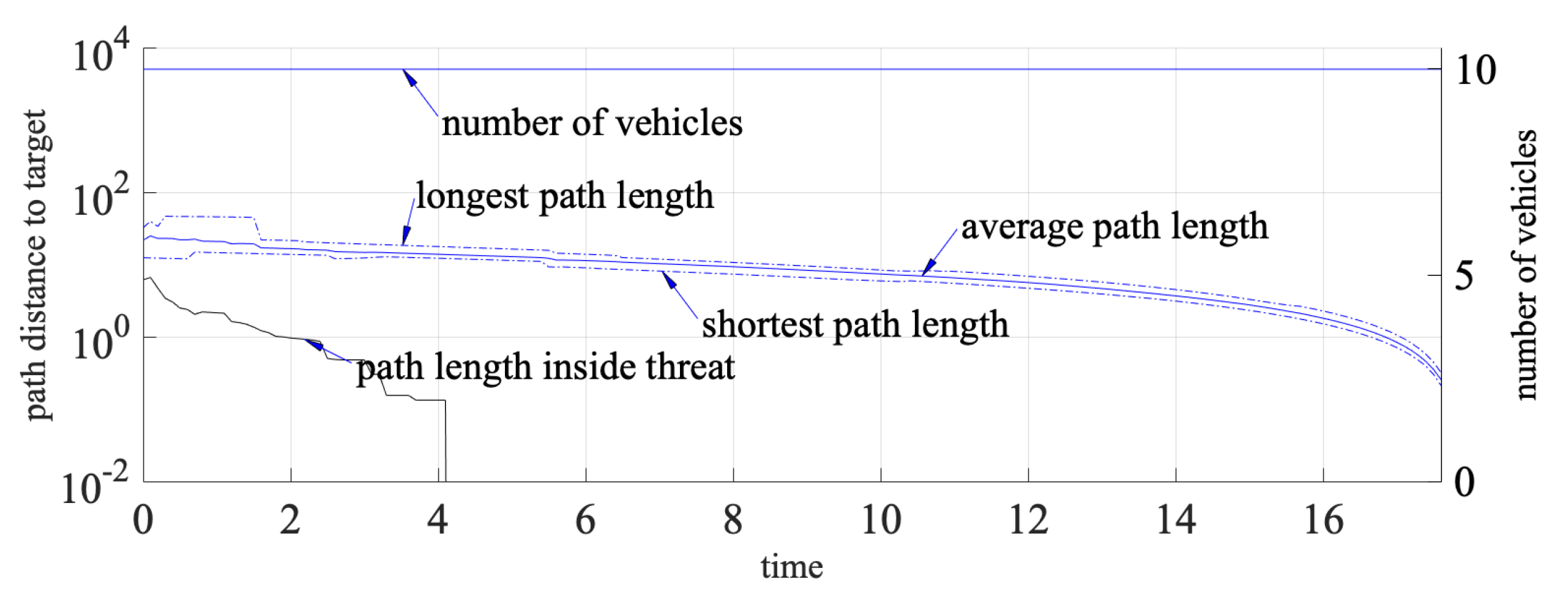
The curves of path lengths and number of vehicles are given in Figure 13, Figure 14 and Figure 15, where there are no communication constraints, and Figure 16, Figure 17 and Figure 18, where there are communication constraints. The curves of path lengths are drawn on a log scale. The overall path lengths reduce steadily, indicating that the vehicles are approaching the target. The path lengths inside threats are also reduced and become zero before the vehicles reach the target. This shows that path-planning algorithms are successful in threat avoidance. The curves of path length inside threats do not indicate the actual track of vehicles inside threats. Take Figure 16 as an example. Around s in the simulation, the curve of path length inside threats jumps from zero to non-zero. However, if we observe Figure 12, the path length inside threats should be zero.

Figure 13.
Curves of path lengths of 4 vehicles and number of vehicles over time without communication constraints.
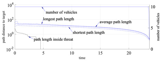
Figure 14.
Curves of path lengths of 10 vehicles and number of vehicles over time without communication constraints.
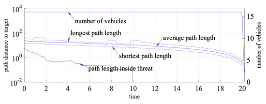
Figure 15.
Curves of path lengths of 16 vehicles and number of vehicles over time without communication constraints.
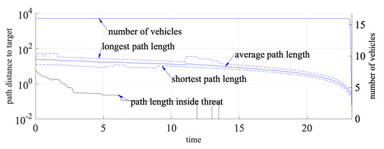
Figure 16.
Curves of path lengths of 16 vehicles and number of vehicles over time with communication constraints.
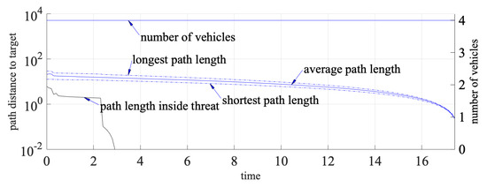
Figure 17.
Curves of path lengths over time with communication constraints.
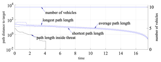
Figure 18.
Curves of path lengths over time with communication constraints.
After a vehicle has reached the target, it will be removed from the group and the number of vehicles will decrease by one. The curves of some vehicles are unchanged throughout most of the simulation and drop to zero as vehicles arrive at the target. This means that the vehicles disappear roughly at the same time. Some vehicles reach the target earlier than others. Then, there is a premature drop that can be observed in Figure 13. At the same time, there is a disturbance in the curves of path lengths. Moreover, due to communication constraints, path updates are less frequent. As a result, disturbances on path length curves in Figure 16, Figure 17 and Figure 18 last longer than those in Figure 13, Figure 14 and Figure 15.
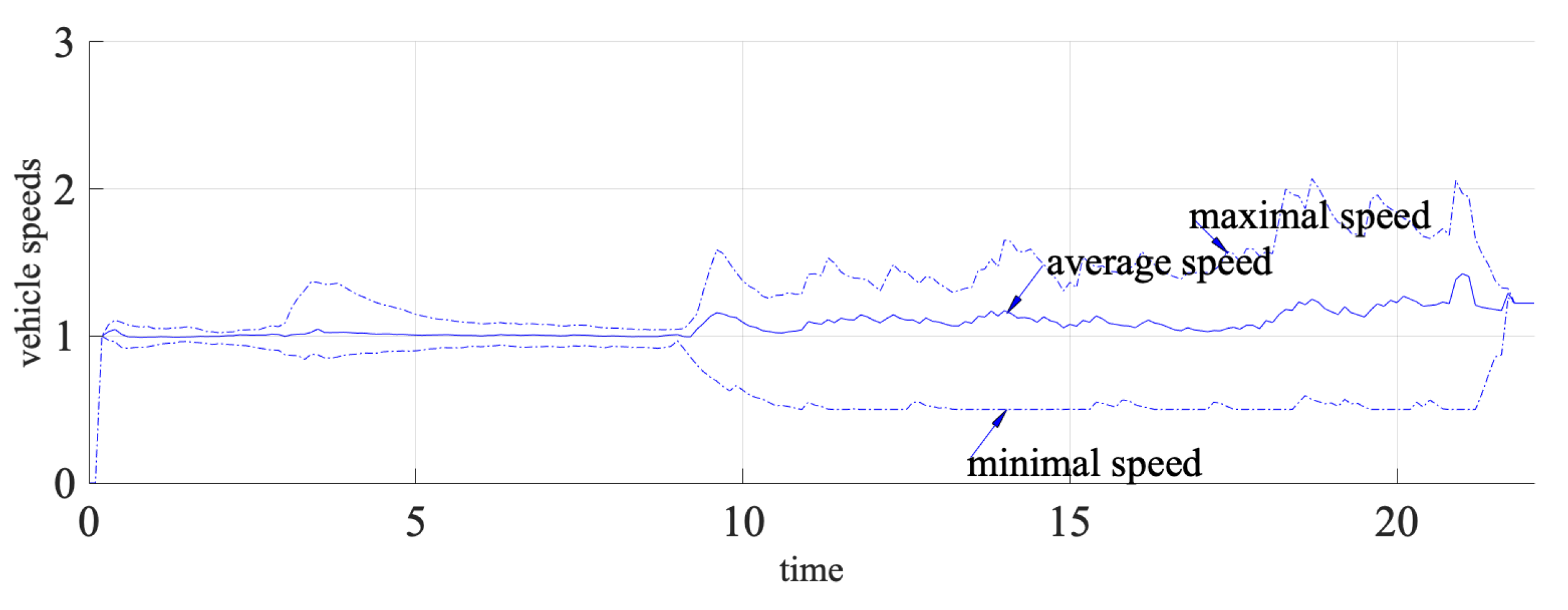
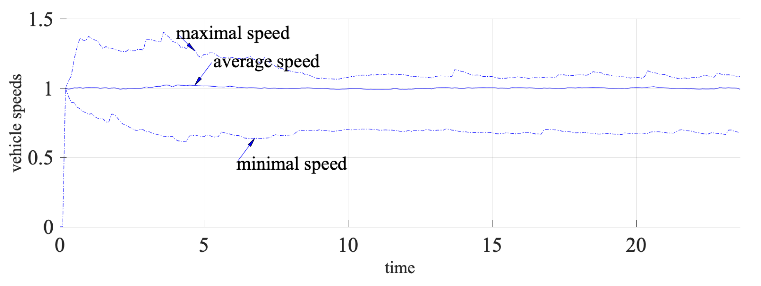
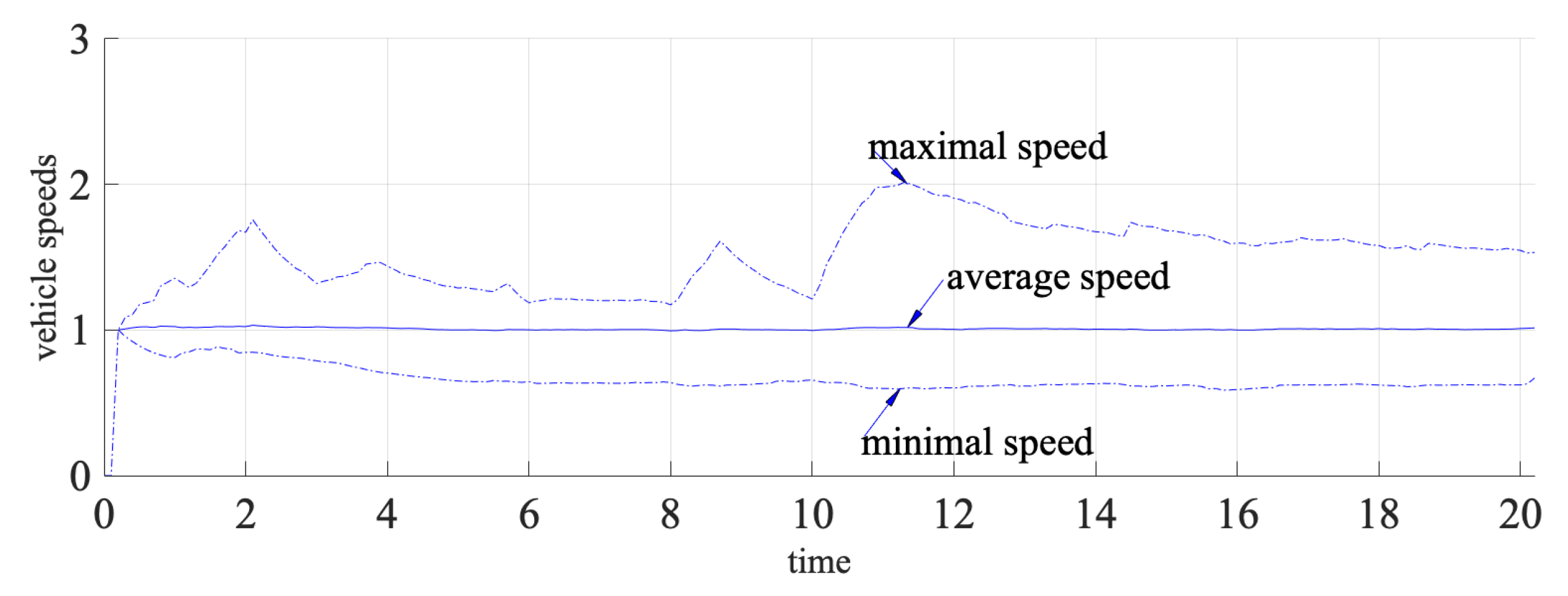
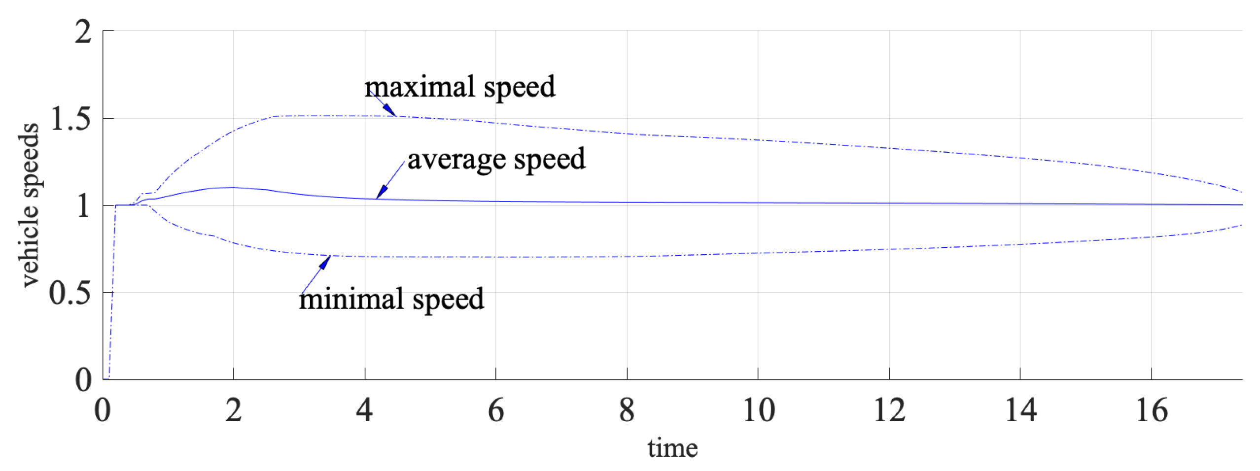
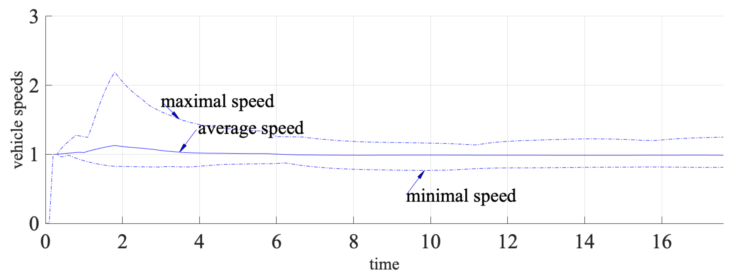
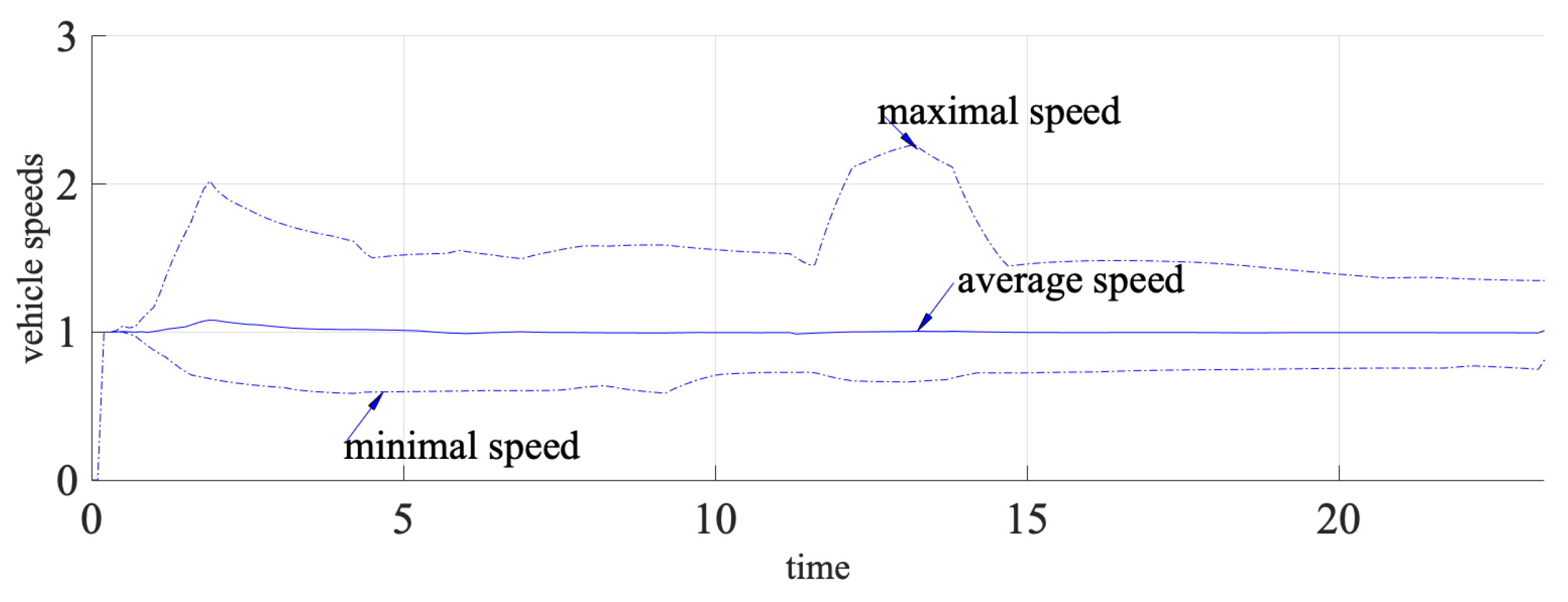
The curves of vehicle speeds are given in Figure 19, Figure 20 and Figure 21, where there are no communication constraints, and Figure 22, Figure 23 and Figure 24, where there are communication constraints. Of all the curves, it is observed that the average speed of all vehicles oscillates around 1. This is because the initial speeds of all vehicles are for any . Ideally, the average speed will remain at 1 throughout the simulations. In practice, average speed oscillations are incurred by erroneous estimation of the average speed from delayed communication and the received paths from other vehicles. This explains why, under communication constraints, the curves in Figure 22, Figure 23 and Figure 24 are smoother than those in Figure 19, Figure 20 and Figure 21, where there are no communication constraints and the frequent path updates lead to frequent speed adjustments by (17).
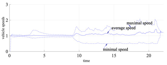
Figure 19.
Curves of speeds of 4 vehicles over time without communication constraints.
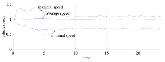
Figure 20.
Curves of speeds of 10 vehicles over time without communication constraints.
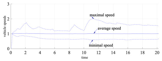
Figure 21.
Curves of speeds of 16 vehicles over time without communication constraints.
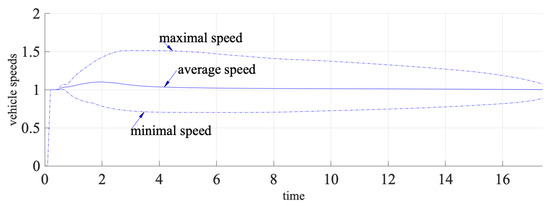
Figure 22.
Curves of speeds of 4 vehicles over time with communication constraints.
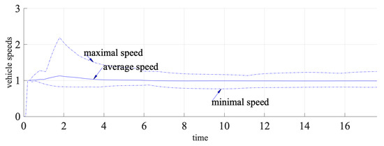
Figure 23.
Curves of speeds of 10 vehicles over time with communication constraints.
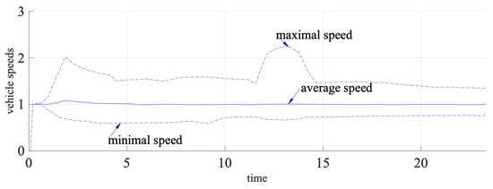
Figure 24.
Curves of speeds of 16 vehicles over time with communication constraints.
The length differences among vehicle paths are the main causes of the speed spikes. They are often observed at the beginning of the simulations when the path difference is most significant or vehicles are taking threat-avoiding actions and underplaying path synchronization. Spikes in speed happen when there is a sudden change in path length. For example, speed oscillations start from s in Figure 19. This happens because a shorter path is found. We can reduce speed oscillation by overplaying the priority for path synchronization.
5. Conclusions
In this paper, we propose an algorithm design for path planning and synchronization for multiple vehicles in the presence of threats. We formulate a cost function to strike a trade-off among path length minimization, threat avoidance, and path length synchronization. Certain Dubins path types and usage cases are considered, which can vary the possible path sequences. A probability-based algorithm is proposed to find the optimal communication frequency and minimal cost function. Vehicles can reach the target simultaneously using real-time commands, while speed and turning radii are controlled within the limit. The performance of the proposed approaches is verified in several simulation examples.
There are several limitations to this study. For example, we consider that targets and threats are static. However, the proposed approaches apply to mobile targets and threats, but this is not the focus of the discussion in this paper. Moreover, they would struggle in threat-dense environments, and pathfinding would be slow and lose real-time responses. For future work, we will investigate a methodology to improve performance when the space is filled with uncertain or dynamic objects. We will look into algorithm designs and change the cost function design to enable vehicles to memorize and learn to handle complicated tasks.
Author Contributions
Conceptualization, methodology, validation, original draft preparation, H.Y.; formal analysis, review and editing, H.Y. and L.Z. All authors have read and agreed to the published version of the manuscript.
Funding
This research was funded by the National Science Foundation of China, grant number 62203133.
Data Availability Statement
Research data will be available upon request.
Conflicts of Interest
The authors declare no conflicts of interest.
References
- Chu, X.; Hu, Q.; Zhang, J. Path Planning and Collision Avoidance for A Multi-Arm Space Maneuverable Robot. IEEE Trans. Aerosp. Electron. Syst. 2017, 54, 217–232. [Google Scholar] [CrossRef]
- Chen, Y.; Cai, Y.; Zheng, J.; Thalmann, D. Accurate and Efficient Approximation of Clothoids Using Bezier Curves for Path Planning. IEEE Trans. Robot. 2017, 33, 1242–1247. [Google Scholar] [CrossRef]
- Bucolo, M.; Buscarino, A.; Famoso, C.; Fortuna, L.; Frasca, M. Control of Imperfect Dynamical Systems. Nonlinear Dyn. 2019, 98, 2989–2999. [Google Scholar] [CrossRef]
- Silva, V.; Siebra, C.; Subramanian, A. Intersections Management for Autonomous Vehicles: A Heuristic Approach. J. Heuristics 2022, 28, 1–21. [Google Scholar]
- Todorovic, M.; Aldakkhelallah, A.; Simic, M. Managing Transitions to Autonomous and Electric Vehicles: Scientometric and Bibliometric Review. World Electr. Veh. J. 2023, 14, 314. [Google Scholar] [CrossRef]
- Wang, J.; Wu, Z.; Yan, S.; Tan, M.; Yu, J. Real-Time Path Planning and Following of a Gliding Robotic Dolphin Within a Hierarchical Framework. IEEE Trans. Veh. Technol. 2021, 70, 3243–3255. [Google Scholar]
- Kannadasan, K.; Edla, D.R.; Kongara, M.C.; Kuppili, V. M-Curves Path Planning Model for Mobile Anchor Node and Localization of Sensor Nodes Using Dolphin Swarm Algorithm. Wirel. Netw. 2020, 26, 2769–2783. [Google Scholar]
- Hayat, S.; Yanmaz, E.; Bettstetter, C.; Brown, T.X. Multi-Objective Drone Path Planning for Search and Rescue with Quality-of-Service Requirements. Auton. Robot. 2020, 44, 1183–1198. [Google Scholar]
- Yanmaz, E.; Balanji, H.; Güven, İ. Dynamic Multi-UAV Path Planning for Multi-Target Search and Connectivity. IEEE Trans. Veh. Technol. 2024, 73, 10516–10528. [Google Scholar] [CrossRef]
- Dutta, S.; Wilde, N.; Smith, S. Informative Path Planning for Active Regression With Gaussian Processes via Sparse Optimization. IEEE Trans. Robot. 2025, 41, 2184–2199. [Google Scholar] [CrossRef]
- Sun, P.; Yu, Z. Tracking Control for A Cushion Robot Based on Fuzzy Path Planning with Safe Angular Velocity. IEEE/CAA J. Autom. Sin. 2017, 4, 610–619. [Google Scholar] [CrossRef]
- Wang, Z.; Zlatanova, S.; van Oosterom, P. Path Planning for First Responders in the Presence of Moving Obstacles with Uncertain Boundaries. IEEE Trans. Intell. Transp. Syst. 2017, 18, 2163–2173. [Google Scholar] [CrossRef]
- Jian, Z.; Zhang, S.; Chen, S.; Nan, Z.; Zheng, N. A Global-Local Coupling Two-Stage Path Planning Method for Mobile Robots. IEEE Robot. Autom. Lett. 2021, 6, 5349–5356. [Google Scholar] [CrossRef]
- Yu, H.; Liu, Y.; Liang, L. Stochastic Control and Time Scheduling for Irregular Robots. J. Frankl. Inst. 2021, 358, 3678–3700. [Google Scholar] [CrossRef]
- Wang, S.; Qin, F.; Tong, Y.; Shang, X.; Zhang, Z. Probabilistic Boundary-Guided Point Cloud Primitive Segmentation Network. IEEE Trans. Instrum. Meas. 2023, 72, 1–13. [Google Scholar] [CrossRef]
- Gu, S.; Chen, G.; Zhang, L.; Hou, J.; Hu, Y.; Knoll, A. Constrained Reinforcement Learning for Vehicle Motion Planning with Topological Reachability Analysis. Robotics 2022, 11, 81. [Google Scholar] [CrossRef]
- Yu, H.; Lim, C.C.; Hunjet, R.; Shi, P. Flocking and Topology Manipulation Based on Space Partitioning. Robot. Auton. Syst. 2020, 124, 103328. [Google Scholar] [CrossRef]
- Qin, H.; Shao, S.; Wang, T.; Yu, X.; Jiang, Y.; Cao, Z. Review of Autonomous Path Planning Algorithms for Mobile Robots. Drones 2023, 7, 211. [Google Scholar] [CrossRef]
- Manyam, S.; Casbeer, D.; Taylor, C. Hybrid Theta: Motion Planning for Dubins Vehicles With Integral Constraints. IEEE Robot. Autom. Lett. 2025, 10, 1497–1504. [Google Scholar] [CrossRef]
- Fu, J.; Sun, G.; Liu, J.; Yao, W.; Wu, L. On Hierarchical Multi-UAV Dubins Traveling Salesman Problem Paths in a Complex Obstacle Environment. IEEE Trans. Cybern. 2024, 54, 123–135. [Google Scholar] [CrossRef]
- Wu, W.; Xu, J.; Sun, Y. Integrate Assignment of Multiple Heterogeneous Unmanned Aerial Vehicles Performing Dynamic Disaster Inspection and Validation Task With Dubins Path. IEEE Trans. Aerosp. Electron. Syst. 2023, 59, 4018–4032. [Google Scholar] [CrossRef]
- Yang, X.; Zhu, X.; Liu, W.; Ye, H.; Xue, W.; Yan, C.; Xu, W. A Hybrid Autonomous Recovery Scheme for AUV Based Dubins Path and Non-Singular Terminal Sliding Mode Control Method. IEEE Access 2022, 10, 61265–61276. [Google Scholar] [CrossRef]
- Tang, L.; Dai, J.; Cheng, Z.; Zhang, H.; Chen, Q. A Digital Twins-Assisted Multi-Autonomous Vehicle Distributed Collaborative Path Planning Algorithm With Fidelity Guarantee. IEEE Trans. Intell. Transp. Syst. 2024, 25, 19904–19916. [Google Scholar] [CrossRef]
- Chang, H.; Liu, Y.; Sheng, Z. Distributed Multi-Agent Reinforcement Learning for Collaborative Path Planning and Scheduling in Blockchain-Based Cognitive Internet of Vehicles. IEEE Trans. Veh. Technol. 2024, 73, 6301–6317. [Google Scholar] [CrossRef]
- Dubins, L.E. On Curves of Minimal Length with A Constraint on Average Curvature, and with Prescribed Initial and Terminal Positions and Tangents. Am. J. Math. 1957, 79, 497–516. [Google Scholar] [CrossRef]


Disclaimer/Publisher’s Note: The statements, opinions and data contained in all publications are solely those of the individual author(s) and contributor(s) and not of MDPI and/or the editor(s). MDPI and/or the editor(s) disclaim responsibility for any injury to people or property resulting from any ideas, methods, instructions or products referred to in the content. |
© 2025 by the authors. Licensee MDPI, Basel, Switzerland. This article is an open access article distributed under the terms and conditions of the Creative Commons Attribution (CC BY) license (https://creativecommons.org/licenses/by/4.0/).