Article

Exploiting a Variable-Sized Map and Vicinity-Based Memory for Dynamic Real-Time Planning of Autonomous Robots

by
Aristeidis Geladaris
1,2,
Lampis Papakostas
1,
Athanasios Mastrogeorgiou
1,3 and
Panagiotis Polygerinos
2,*
1
Tech Hive Labs, 11855 Athens, Greece
2
Control Systems and Robotics Lab (CSRL), Mechanical Engineering Department, School of Engineering, Hellenic Mediterranean University, 71004 Heraklion, Greece
3
Control Systems Lab (CSL), School of Mechanical Engineering, National Technical University of Athens, 15773 Athens, Greece
*
Author to whom correspondence should be addressed.
Robotics 2025, 14(4), 44; https://doi.org/10.3390/robotics14040044
Submission received: 27 February 2025 / Revised: 24 March 2025 / Accepted: 27 March 2025 / Published: 31 March 2025
(This article belongs to the Section Aerospace Robotics and Autonomous Systems)

Abstract

:
This paper presents a complete system for autonomous navigation in GPS-denied environments using a minimal sensor suite that operates onboard a robotic vehicle. Our system utilizes a single camera and, given a target destination without prior knowledge of the environment, replans in real time to generate a collision-free trajectory that avoids static and dynamic obstacles. To achieve this, we introduce, for the first time, a local Euclidean Signed Distance Field (ESDF) map with variable size and resolution, which scales as a function of the vehicle’s velocity. The map is updated at a high rate, requiring minimal computational power. Additionally, a short-term vicinity-based memory is maintained for previously observed areas to facilitate smooth trajectory generation, addressing the limited field-of-view provided by the RGB-D camera. System validation is carried out by deploying our algorithm on a differential drive vehicle in both simulation and real-world experiments involving static and dynamic obstacles. We benchmark our robotic system against state-of-the-art autonomous navigation frameworks, successfully navigating to designated target locations while avoiding obstacles in both static and dynamic scenarios, all without introducing additional computational overhead. Our approach consistently achieves the target goals even in complex settings where current state-of-the-art methods may fall short.

1. Introduction

The way a robot perceives its environment is crucial for autonomous navigation, exploration, and task completion. The increasing use of autonomous robotic vehicles in industrial applications requires safe operation in unstructured, dynamic, and human-populated environments, often without prior knowledge. In such scenarios, conventional localization systems like GPS can be unreliable for providing accurate navigational information [1]. This need guides research endeavors to develop real-time motion planning algorithms that can handle complex and dynamic environments without prior knowledge of the map while executing computational tasks onboard. Developing such a system involves integrating four core components: localization, obstacle detection, trajectory generation, and trajectory tracking. The need for onboard, real-time processing necessitates lightweight frameworks that efficiently discard abundant information.
The advantages of Euclidean Signed Distance Fields (ESDFs) for local trajectory planning are widely recognized [2,3], as their volumetric maps offer dynamic updating and accurate representation of complex environments, enabling real-time mapping and localization in dynamic environments [4,5,6]. However, these methods add computational overhead to large-scale navigation scenarios. To tackle these challenges, certain methods resort to the use of distance information from a Truncated Signed Distance Field (TSDF) map [7], gradient information that does not require the generation of an ESDF map [8], occupancy grid maps [9], or simpler data structures like a 3D circular buffer [10], leading to suboptimal or incomplete paths and inefficiency in complex or dynamic environments. To address these limitations, adaptive-size data structures have also been employed to represent the robot’s environment across multiple layers with different voxel sizes [11,12,13,14]. This approach aims to achieve detailed representations without excessive computational cost. However, these methods are typically optimized based on the characteristics of the environment and the sensors used, rather than the requirements of a moving robotic system. Consequently, they cannot be seamlessly integrated with path planning methods.
In addition, discretizing the environment into a grid often leads to search-based solutions on path planning [8,15,16,17,18]. However, these methods may become inefficient in large or cluttered environments and often struggle with dynamic settings. Optimization-based algorithms, such as [10,19], aim to minimize a cost function defined by constraints and preferences and can offer adaptability to different scenarios and the generation of smooth and continuous paths, but this comes at high computational costs, particularly in real-time applications.
This paper aims to present a complete system for autonomous navigation in GPS-denied environments, able to generate collision-free trajectories in real time in both static and dynamic environments (Figure 1). It employs a minimal sensor suite, relying on a stereo camera for all of the robot’s sensing needs [20]. In addition, it is completely autonomous, since all required computational tasks are executed onboard. To achieve this, we create a local map containing the necessary information for path planning and discard unused information to minimize computational power. We summarize our key contributions as follows:
  • A unified autonomous navigation system that dynamically adapts to complex environments with robust obstacle avoidance. Its low computational overhead enables onboard processing for visual odometry, local mapping, and trajectory planning without requiring prior knowledge of the environment or reliance on complex sensors.
  • An innovative, adaptive local ESDF map that dynamically adjusts its size and resolution based on vehicle velocity, enabling high-frequency updates for efficient and responsive path planning.
  • A novel mechanism combining adaptive offset map positioning based on angular velocity and short-term map memory to retain information from previously observed areas at the vicinity of the robot, minimizing redundant calculations and preventing unnecessary maneuvers.
The work is organized as follows: Section 2 discusses the mapping and path planning algorithms used to navigate the robot. Section 3 describes the robotic vehicle used for real-world experiments. Section 4 presents experimental results in simulation and real-world environments. Finally, Section 5 offers conclusions and discussions for future directions.

2. Mapping and Path Planning Algorithm

2.1. Local Mapping

This work builds upon the approach described in [6], but we focus on maximizing the update rate of the generated map. To achieve this, we limit the creation of a global ESDF map to a submap of the robot’s surroundings, effectively reducing the computational overhead by excluding redundant information that is not required for the replanning process. The map’s high update rate enables real-time replanning in dynamic environments without relying on predictive or velocity-based models. To ensure that no valuable spatial data are lost, a trade-off mechanism between the represented area’s size and the map’s resolution is introduced. Unlike existing ESDF-based approaches that maintain static grid resolutions, this mechanism adopts a variable sized map approach where the map’s covering area is dynamically scaled based on the vehicle’s velocity. Specifically, the dimensions of the map along the x- and y-axes scale proportionally to the velocity, while the resolution is adapted accordingly to maintain a high update rate. As a result, the map’s resolution increases when velocity is low to accommodate precise path planning in spaces with narrow passages and increases at higher-velocities to effectively facilitate path planning.
Map Size: To adjust the size of the map, we follow the assumption that the trajectory replanning algorithm has a number of N control points with a fixed time interval d t where the robot would need occupancy information in a horizon of x m a p = N × d t × V x , where V x is the velocity of the robot, considering a constant velocity. Setting a safety factor S to ascertain that the mapped area maintains sufficient information of the surroundings, the length of the map along the x-axis is as follows:
x p l a n n e d = S × N × d t × V x
where x ϵ [ x m i n , x m a x ] , x m i n 0 to avoid a null map at zero velocities.
To replan around obstacles when moving at higher velocities, the map must depict the space where the robot can safely execute maneuvers. To accomplish this, the map’s size along the y-axis is also adjusted based on the vehicle’s linear velocity. However, blind spots are encountered during trajectories with a change in curvature often leading to missing out useful trajectory information. To avoid those blind spots, we introduce a lateral offset to the map. The amount of the offset provided is determined by the robot’s angular velocity (see Equation (2)). This adaptive behavior allows the robot to maintain, for a longer duration, that part of the visual information on the map. This could be compared to the left or right adaptive headlights offered in modern automobiles, which detect the steering angle and light up accordingly to illuminate the trajectory of the car only during the turning maneuver. In our algorithm, the y-coordinate of the map center can be calculated based on the size of the map and the angular velocity as
y c = ω ω m a x y m a p
Resolution: The generated map divides the indicated 3D space into voxels to determine occupancy. The number of these voxels N v is
N v = x m a p × y m a p × z m a p / r e s 3
The number of voxels regulates the map update time, and, therefore, to maintain the map update frequency high, the map’s resolution decreases according to its size. With this approach, the map offers a finer representation of the robot’s surroundings for low-velocity motions, allowing path planning through narrow spaces. In higher velocities, the vehicle provides a coarse, but extensive, representation of the environment to avoid collisions with static and dynamic obstacles.
Given that the camera generates point clouds within a conical sector due to its field of view, the updated area of the map is limited. To maintain simplicity and cost-effectiveness, we avoid using additional cameras or expensive 3D LiDAR sensors. Instead, we adopt a short-term vicinity-based memory area to extend the information on the map without compromising the ability to handle dynamic environments through constant updates. The previously observed information is not updated within this area to minimize unnecessary maneuvers and non-smooth trajectories. Additionally, the updated area is approximated using three rectangular boxes (two constant-sized and one variable-sized), as shown in Figure 2 to approximate the near conical shape of the point cloud close to the camera (see Figure 3).
The occupancy update algorithm of Algorithm 1 consists of two loops. The first loop ensures that voxels that are no longer in range, but were previously observed, are still marked as occupied. The second loop updates the map based on new sensor data, managing voxels that need to be added or eliminated. The ESDF update algorithm (Algorithm 2) handles inserting and deleting voxels in the map using two independent queues while managing distances to the nearest obstacle. Figure 3 shows a map created from our system during our experiments with an unmanned ground vehicle (UGV) (see Section 3).
Algorithm 1 Occupancy update algorithm
  • for each  v o x   in  m e m o r y _ r a n g e   do
  •    i d x V o x T o I d x ( v o x )
  •   if  E x i s t ( i d x )  and not  I n R a n g e ( i d x )  then
  •      o c c u p a n c y ( i d x ) 1
  •      d i s t a n c e ( i d x ) 0
  •   else
  •      o c c u p a n c y ( i d x ) u n d e f i n e d
  •      d i s t a n c e ( i d x ) I n f
  •   end if
  • end for
  • for each  p o i n t   in  n e w _ p o i n t c l o u d _ m s g   do
  •    i d x P n t T o I d x ( p o i n t )
  •    o c c u p i e d E x i s t ( i d x )
  •   if ( I n R a n g e ( i d x ) then
  •      o c c u p a n c y ( i d x ) 1
  •      d i s t a n c e ( i d x ) 0
  •   end if
  •    v o x I d x T o V o x ( i d x )
  •   if ( E x i s t ( i d x )  and not  o c c u p i e d then
  •      i n _ q u e u e . push( v o x )
  •   else if (not  E x i s t ( i d x )  and  o c c u p i e d then
  •      o u t _ q u e u e . push( v o x )
  •   end if
  • end for
Algorithm 2 ESDF update algorithm
  • for each  v o x   in  i n s e r t _ q u e u e   do
  •    i d x V o x T o I d x ( v o x )
  •    c l o s e s t _ o b s t ( i d x ) v o x
  •    d i s t a n c e ( i d x ) 0
  •    u p d a t e _ q u e u e . push( v o x )
  • end for
  • for each  v o x   in  d e l e t e _ q u e u e   do
  •    i d x V o x T o I d x ( v o x )
  •    d i s t a n c e ( i d x ) I n f
  •   for each  n e i g h b o u r  in  n e i g h b o u r s ( i d x )  do
  •      n _ i d x V o x T o I d x ( n e i g h b o u r )
  •      t m p E u c l D i s t ( n _ i d x , i d x ) + d i s t a n c e ( n _ i d x )
  •     if ( t m p < d i s t a n c e ( i d x ) then
  •        d i s t a n c e ( i d x ) t m p
  •        c l o s e s t _ o b s t ( i d x ) c l o s e s t _ o b s t ( n _ i d x )
  •     end if
  •   end for
  • end for

2.2. Path Planning

Our approach uses an optimization-based local trajectory replanning algorithm [10], which, given a global path, will lead to obstacle avoidance utilizing gradient information from the ESDF map with minimum deviation from the given path through the minimization of the cost function L of Equation (4). To reduce the computation time of the optimization framework, we simplify the cost function by incorporating only the essential terms required to ensure a feasible, collision-free path while avoiding unnecessary maneuvers. The points generated by this optimization process serve as the control points of a B-Spline trajectory, which reduces the optimization time by minimizing the number of constraints needed in the optimization process. Additionally, the B-Splines’ inherent ability to generate smooth trajectories and their advantageous property of local control are essential for real-time replanning in dynamic environments [21].
L = L c + L e p + L s
The cost function consists of a collision term (Equation (5)) that penalizes the paths that lead to a collision, an endpoint error term (Equation (6)) used to maintain the replanned trajectory as close to the initial one as possible, and a soft limit (Equation (7)) used to maintain the velocity, acceleration and jerk values bounded and that allows the use of an unconstrained optimization algorithm.
L c = λ c t i t f ( d i f f ( t ) ) 2 d t
where:
d i f f ( t ) = 0 if d ( t ) τ > 0 d ( t ) τ if d ( t ) τ 0
λ c is a weight parameter, d ( t ) is the distance to the nearest obstacle calculated using trilinear interpolation from the incrementally built ESDF map, and τ is a user-defined threshold.
L e p = λ p | | p g l o b ( t f ) p ( t f ) | | 2 + λ v | | v g l o b ( t f ) v ( t f ) | | 2
λ i are weight parameters for the position and velocity terms; p g l o b ( t f ) and v g l o b ( t f ) are the desired position and velocity, respectively, at the end of the time segment; and p ( t f ) and v ( t f ) are the position and velocity, respectively, at the end of the segment of the B-Spline.
L s = n = 2 n = 4 t i t f b ( t , i ) d t
where
b ( t , i ) = 0 if p ( i ) ( t ) p m a x ( i ) e x p ( ( p ( i ) ( t ) ) 2 ( p m a x ( i ) ) 2 ) if p ( i ) ( t ) > p m a x ( i )
p ( i ) ( t ) is the i-th derivative of the position at time t and p m a x ( i ) is the limit value.
For the optimization problem, an open-source library for nonlinear optimization, the NLopt [22], is adopted.

3. The Developed UGV

3.1. Hardware

The UGV used for the experiments is the differential drive vehicle in Figure 4. The robot’s chassis consists of the power management cabinet containing the batteries with the power management board and the electronics cabinet with the onboard computer, the motor drivers, and the camera. The onboard computer is a Jetson Xavier with a 6-core NVIDIA Carmel ARM CPU (Nvidia, Santa Clara, CA, USA). At the front of the vehicle, a ZEDX mini camera [23] (ZEDX, Bellefonte, PA, USA) with a 2.2 mm focal length is integrated for visual odometry and point cloud generation with a depth range of 0.1–8 m & an update rate of up to 30 Hz.
The front wheels are independently controlled, while the rear are passive caster wheels. The active front wheels (ODrive BotWheels [24]) are a combination of brushless wheel hub motors with hall sensors and a high-resolution (3200 CPR) integrated reflecting encoder. The motors can continuously produce a torque of 5 Nm. A CAN controller operating at a 250 kbps bitrate is used to send velocity commands to the motor drivers (ODrive S1 [25]) from the onboard computer to control the wheels.
The vehicle dimensions are 430 mm × 400 mm × 300 mm and the maximum velocity is 0.985 m/s. Two 4S Li-ion batteries (14.8 V, 18 Ah) connected in series power the UGV.

3.2. Control

The optimization process for local path replanning produces an output of control points that define the robot’s trajectory. Although the number of the computed control points is defined and maintained throughout the vehicle’s motion, their coordinates are computed every time the vehicle reaches the next control point in the sequence until the robot reaches its final destination. To ascertain that the robot can accurately traverse all the control points generating a smooth trajectory, a tracking PID controller is adopted [26]. This approach offers a tuneable PID control loop, where the robot’s base link tracks a projected point (PP) on the generated trajectory at a fixed distance l ahead of the robot. The PID gains are empirically tuned through an iterative process to ensure a smooth trajectory, minimizing overshoot and achieving zero steady-state error. This PP traverses the path between two control points at a constant velocity, with longitudinal and angular errors used as control feedback to compute the vehicle’s velocity. As the robot approaches the next control point within a distance threshold, the subsequent control point is incorporated into the desired trajectory. By keeping l sufficiently smaller than the threshold distance, the vehicle is able to follow a smooth trajectory. The controller continuously updates the path with each new control point until the robot reaches its final destination. For our application, PP is set at l = 0.1 m ahead of the vehicle and moves at a velocity of 0.3 m/s.
The differential drive dynamics of the vehicle are incorporated into the controller, and the controller gains are adjusted through an iterative tuning process to further improve the vehicle’s performance during path tracking. The PI gains of the ODrive controller that controls the wheels of the robotic platform are similarly tuned to minimize overshoot and to ensure the precise tracking of velocity commands.

4. Experimental Results

4.1. Simulation Experiments

To test the stability of the proposed method, the vehicle is required to navigate avoiding obstacles—static or dynamic—randomly placed in simulated environments generated using Gazebo-11.12, run on a 2.6 GHz Intel i7 CPU with 16 GB RAM (Intel, Santa Clara, CA, USA). The virtual robotic vehicle model employed (Figure 5a) is a differential drive UGV that implements the controller approach described in Section 3.2, and its mass properties are derived from a computer-aided design of the vehicle in Section 3.1 and cross-referenced using the fabricated prototype. The point cloud data are generated by [27] and are parameterized to match the ZED X mini camera. Pedestrian models crossing the robot’s planned path are added using the pedsim_ros library [28], and odometry data are provided by [29]. Simulation experiments are carried out in an indoor environment with random static and dynamic obstacles creating narrow passages, such as the one presented in Figure 5a and in a large-scale dynamic environment.
To benchmark our approach, we compare it with three state-of-the-art open-source approaches for autonomous navigation, restricting them to perform path planning exclusively in 2D: FAST-Planner [30], EWOK [10], and FAEL [31]. The first uses kinodynamic path searching with a B-spline-based trajectory optimized over the Euclidean Distance Fields of a voxel map. The second is an optimization-based path planning method used to replan in cluttered environments with static obstacles, and the latter uses a probabilistic 3D grid map with a search-based approach for planning and is optimized for UGVs. We compare the frameworks on the optimization time, map update time, path length, and success ratio. While FAEL is optimized for large-scale exploration, we adapt it for direct goal-reaching tasks. Similarly, FAST-Planner, although designed for UAV navigation, shares ESDF-based optimization principles and is evaluated in a 2D setting. EWOK, which assumes static environments, provides a baseline for testing dynamic obstacle handling. To evaluate the map update and optimization time, we use Scalopus [32], a tracing framework, to obtain traces for each scope of interest (Figure 5b). The utilized profiling tool visualizes the time spent in annotated sections of the code or function call frames. It uses a browser-based trace viewer, displaying performance data in a way that is easy to interpret.
We initially compare our approach to all methods regarding the duration of the optimization process before each path replanning. As shown in Figure 6, FAST-Planner demonstrates the fastest optimization times, with our proposed method following closely, showing a difference of approximately 20 ms. The longer duration values observed in FAEL can be attributed to its design for large-scale environmental exploration, which requires tracking unexplored areas.
The assumption of EWOK of a static environment, which results in inaccurate maps in dynamic scenarios, led us to exclude it from comparing the map update time. The results in Figure 7 show minor differences in the update times of the maps between the methods, reasonable considering the variations in their map generation approaches. For comparison methods that require a predefined resolution and known map size, these parameters are set to the median of the minimum and maximum values used in our approach: resolution = 0.1 m, map_size = 5.5 m × 5.5 m × 4 m.
As FAEL is primarily designed for autonomous exploration rather than guiding a robot to a specific goal and EWOK cannot handle dynamic obstacles during map updates, we excluded them and focused our evaluation on comparing our approach with FAST-Planner, a state-of-the-art method for autonomous navigation in dynamic environments. Table 1 presents the normalized path lengths generated by our approach and FAST for successful indoor experiments (S: static; D: dynamic). The results demonstrate that the path lengths are highly comparable and close to the initial path, indicating that unnecessary maneuvers are avoided and near-optimal paths are produced.
FAST-Planner employs a hybrid method, creating an optimized replanned path over an A*-generated initial guess, which minimizes the duration of the optimization time. However, this approach has certain disadvantages in specific scenarios. For example, dense and narrow corridors (Figure 8a) and winding paths with dead ends (Figure 8b) can make A* less efficient, as it can explore numerous paths before finding the correct one. Furthermore, sparse obstacles that require long detours (Figure 8c) can significantly slow the process, potentially leading to failures to reach the target location. In all the experimental setups of Figure 8, using the same parameters for map generation, the FAST-Planner approach always fails to reach the goal point, while our approach shows success with scores greater than 0.8 for all scenarios (as shown in Table 2). This is largely due to the incorporation of constraints regarding vehicle dynamics directly into the optimization process in our method.

4.2. Real-World Experiments

We evaluate our system on the UGV prototype (Section 3) in several indoor experiments. To keep our system computationally light and avoid unnecessary onboard processing, we restrict from using an open-source pose estimator and use the positional tracking module of the ZEDX mini stereo camera [33].
In these experiments, the vehicle operates without prior knowledge of the map and is assigned a target destination. Using only a stereo camera for localization, mapping, and path following, the vehicle successfully navigates towards the goal, avoiding static objects and randomly walking pedestrians encountered along its path. All computations are executed onboard using an embedded computer system (Jetson Xavier, NVidia), allowing the robotic vehicle to consistently avoid obstacles and reach the goal position in all experiments. Throughout the real-world experiments, various configurations involving both static and dynamic obstacles within an indoor corridor are employed (Figure 9).
The mean optimization time was recorded at 116.9 ms, with the map update time averaging 92.3 ms. These values are higher compared to simulation results, primarily because the embedded computer offers lower computational power relative to the system used to perform the simulations. Subsequently, a densely cluttered environment featuring dead ends (similar to the one in Figure 8b) was constructed to evaluate the performance of our approach in comparison to FAST-Planner. As shown in Figure 10, our method successfully guided the robot to the target, while FAST-Planner failed to complete the path.

5. Discussion

We introduced a novel autonomous navigation approach capable of handling unstructured and dynamic environments. Using distance information from a newly developed variable-sized ESDF map, the robot can reach its target destination by generating a smooth, B-spline-based trajectory through optimization. Unlike fixed ESDF methods, our approach maintains computational efficiency while adapting to the vehicle’s motion state. The system was validated in simulated environments and on a custom mobile robotic platform equipped with a minimum sensor suite in various indoor scenarios, specifically using only a stereo camera for all sensing needs. Our approach is benchmarked against state-of-the-art autonomous navigation methods in complex static and dynamic environments. Although our system incurs slightly higher computational overhead compared to FAST-Planner, it consistently demonstrates robustness and efficiency in reaching the target position, even in highly challenging scenarios where existing algorithms fail to complete the course.
In the future, we plan to deploy our system in a heterogeneous robotic swarm consisting of both ground and aerial vehicles. This will allow us to validate the transferability of the parameterized software across various types of robotic platforms, enabling robust task execution in even more complex and dynamic scenarios.

Supplementary Materials

The following supporting information can be downloaded: https://www.mdpi.com/article/10.3390/robotics14040044/s1.

Author Contributions

Conceptualization, A.G., L.P., A.M. and P.P.; methodology, A.G. and L.P.; software, A.G. and L.P.; validation, A.G. and A.M.; formal analysis, A.G. and L.P.; investigation, A.G.; resources, A.M. and P.P.; data curation, A.G. and L.P.; writing—original draft preparation, A.G. and A.M.; writing—review and editing, P.P.; visualization, A.G., A.M. and P.P.; supervision, A.M. and P.P.; project administration, A.M. and P.P.; funding acquisition, A.M. and P.P. All authors have read and agreed to the published version of the manuscript.

Funding

This research has been co-financed by the European Union NextGenerationEU project under the call RESEARCH–CREATE–INNOVATE 16971 Recovery and Resilience Facility (project: ENORASI, code: TAEDK-06172).

Data Availability Statement

Data is contained within the article and Supplementary Materials.

Conflicts of Interest

Authors Aristeidis Geladaris, Lampis Papakostas and Athanasios Mastrogeorgiou were employed by the company Tech Hive Labs. The remaining author declares that the research was conducted in the absence of any commercial or financial relationships that could be construed as a potential conflict of interest.

Abbreviations

The following abbreviations are used in this manuscript:
GPSGlobal Positioning System
ESDFEuclidean Signed Distance Field
RGB-DRed Green Blue–Depth
TSDFTruncated Signed Distance Field
3DThree-Dimensional
LiDARLight Detection And Ranging
UGVUnmanned Ground Vehicle
CPUCentral Processing Unit
CPRCounts Per Revolution
CANController Area Network
PIDProportional–Integral–Derivative
PPProjected Point
RAMRandom-Access Memory

References

  1. Lu, Z.; Liu, F.; Lin, X. Vision-based localization methods under GPS-denied conditions. arXiv 2022, arXiv:cs.CV/2211.11988. [Google Scholar]
  2. Gao, F.; Wang, L.; Zhou, B.; Zhou, X.; Pan, J.; Shen, S. Teach-Repeat-Replan: A Complete and Robust System for Aggressive Flight in Complex Environments. IEEE Trans. Robot. 2020, 36, 1526–1545. [Google Scholar] [CrossRef]
  3. Oleynikova, H.; Taylor, Z.; Siegwart, R.; Nieto, J. Safe Local Exploration for Replanning in Cluttered Unknown Environments for Micro-Aerial Vehicles. IEEE Robot. Autom. Lett. 2017, 3, 1474–1481. [Google Scholar] [CrossRef]
  4. Hornung, A.; Wurm, K.; Bennewitz, M.; Stachniss, C.; Burgard, W. OctoMap: An efficient probabilistic 3D mapping framework based on octrees. Auton. Robot. 2013, 34, 189–206. [Google Scholar] [CrossRef]
  5. Oleynikova, H.; Taylor, Z.; Fehr, M.; Siegwart, R.; Nieto, J. Voxblox: Incremental 3D Euclidean Signed Distance Fields for on-board MAV planning. In Proceedings of the 2017 IEEE/RSJ International Conference on Intelligent Robots and Systems (IROS), Vancouver, BC, Canada, 24–28 September 2017; pp. 1366–1373. [Google Scholar] [CrossRef]
  6. Han, L.; Gao, F.; Zhou, B.; Shen, S. FIESTA: Fast Incremental Euclidean Distance Fields for Online Motion Planning of Aerial Robots. In Proceedings of the 2019 IEEE/RSJ International Conference on Intelligent Robots and Systems (IROS), Macau, China, 3–8 November 2019; pp. 4423–4430. [Google Scholar] [CrossRef]
  7. Oleynikova, H.; Lanegger, C.; Taylor, Z.; Pantic, M.; Millane, A.; Siegwart, R.; Nieto, J. An open-source system for vision-based micro-aerial vehicle mapping, planning, and flight in cluttered environments. J. Field Robot. 2020, 37, 642–666. [Google Scholar] [CrossRef]
  8. Zhou, X.; Wang, Z.; Ye, H.; Xu, C.; Gao, F. EGO-Planner: An ESDF-free Gradient-based Local Planner for Quadrotors. IEEE Robot. Autom. Lett. 2020, 6, 478–485. [Google Scholar] [CrossRef]
  9. Tordesillas, J.; How, J.P. FASTER: Fast and Safe Trajectory Planner for Navigation in Unknown Environments. IEEE Trans. Robot. 2021, 38, 922–938. [Google Scholar]
  10. Usenko, V.; von Stumberg, L.; Pangercic, A.; Cremers, D. Real-time trajectory replanning for MAVs using uniform B-splines and a 3D circular buffer. In Proceedings of the 2017 IEEE/RSJ International Conference on Intelligent Robots and Systems (IROS), Vancouver, BC, Canada, 24–28 September 2017; pp. 215–222. [Google Scholar] [CrossRef]
  11. Yuan, C.; Xu, W.; Liu, X.; Hong, X.; Zhang, F. Efficient and Probabilistic Adaptive Voxel Mapping for Accurate Online LiDAR Odometry. IEEE Robot. Autom. Lett. 2022, 7, 8518–8525. [Google Scholar] [CrossRef]
  12. Wang, W.; Hu, Y.; Xi, W.; Zou, D.; Yu, W. Efficient Semantic-Aware TSDF Mapping with Adaptive Resolutions. In Proceedings of the 2023 3rd International Conference on Robotics, Automation and Artificial Intelligence (RAAI), Singapore, 14–16 December 2023; pp. 39–45. [Google Scholar] [CrossRef]
  13. Funk, N.; Tarrio, J.; Papatheodorou, S.; Popović, M.; Alcantarilla, P.F.; Leutenegger, S. Multi-Resolution 3D Mapping with Explicit Free Space Representation for Fast and Accurate Mobile Robot Motion Planning. IEEE Robot. Autom. Lett. 2021, 6, 3553–3560. [Google Scholar] [CrossRef]
  14. Zheng, J.; Barath, D.; Pollefeys, M.; Armeni, I. Map-adapt: Real-time quality-adaptive semantic 3D maps. In European Conference on Computer Vision; Springer: Cham, Switzerlad, 2025; pp. 220–237. [Google Scholar]
  15. Bircher, A.; Kamel, M.; Alexis, K.; Oleynikova, H.; Siegwart, R. Receding Horizon “Next-Best-View” Planner for 3D Exploration. In Proceedings of the 2016 IEEE International Conference on Robotics and Automation (ICRA), Stockholm, Sweden, 16–21 May 2016; pp. 1462–1468. [Google Scholar] [CrossRef]
  16. Nieuwenhuisen, M.; Beul, M.; Droeschel, D.; Behnke, S. Obstacle Detection and Navigation Planning for Autonomous Micro Aerial Vehicles. In Proceedings of the 2014 International Conference on Unmanned Aircraft Systems, ICUAS 2014—Conference Proceedings, Orlando, FL, USA, 27–30 May 2014. [Google Scholar] [CrossRef]
  17. Mohta, K.; Watterson, M.; Mulgaonkar, Y.; Liu, S.; Qu, C.; Makineni, A.; Saulnier, K.; Sun, K.; Zhu, A.; Delmerico, J.; et al. Fast, Autonomous Flight in GPS-Denied and Cluttered Environments. J. Field Robot. 2017, 35, 101–120. [Google Scholar] [CrossRef]
  18. Burri, M.; Oleynikova, H.; Achtelik, M.W.; Siegwart, R. Real-time visual-inertial mapping, re-localization and planning onboard MAVs in unknown environments. In Proceedings of the 2015 IEEE/RSJ International Conference on Intelligent Robots and Systems (IROS), Hamburg, Germany, 28 September–2 October 2015; pp. 1872–1878. [Google Scholar] [CrossRef]
  19. Zhou, B.; Pan, J.; Gao, F.; Shen, S. RAPTOR: Robust and Perception-Aware Trajectory Replanning for Quadrotor Fast Flight. IEEE Trans. Robot. 2021, 37, 1992–2009. [Google Scholar] [CrossRef]
  20. Geladaris, A.; Papakostas, L.; Mastrogeorgiou, A.; Sfakiotakis, M.; Polygerinos, P. Real-Time Local Map Generation and Collision-Free Trajectory Planning for Autonomous Vehicles in Dynamic Environments. In Proceedings of the 2023 International Conference on Control, Artificial Intelligence, Robotics & Optimization (ICCAIRO), Crete, Greece, 11–13 April 2023; pp. 1–6. [Google Scholar] [CrossRef]
  21. Zuo, K.; Cheng, X.; Zhang, H. Overview of Obstacle Avoidance Algorithms for UAV Environment Awareness. J. Phys. Conf. Ser. 2021, 1865, 042002. [Google Scholar] [CrossRef]
  22. Johnson, S.G. The NLopt Nonlinear-Optimization Package. 2007. Available online: https://github.com/stevengj/nlopt (accessed on 15 January 2024).
  23. StereoLabs. ZED X. 2024. Available online: https://www.stereolabs.com/en-gr/products/zed-x (accessed on 20 November 2023).
  24. ODriveRobotics. ODrive BotWheels. 2024. Available online: https://odriverobotics.com/shop/botwheels (accessed on 29 August 2023).
  25. ODriveRobotics. ODrive S1 Datasheet. 2024. Available online: https://docs.odriverobotics.com/v/latest/hardware/s1-datasheet.html (accessed on 29 August 2023).
  26. Michiel Franke, C.L. Tracking_pid. 2020. Available online: https://github.com/nobleo/tracking_pid (accessed on 19 December 2023).
  27. PAL-Robotics. Intel RealSense Gazebo ROS Plugin. 2019. Available online: https://github.com/pal-robotics/realsense_gazebo_plugin (accessed on 23 January 2024).
  28. Billy Okal, T.L. Pedestrian Simulator. 2014. Available online: https://github.com/srl-freiburg/pedsim_ros (accessed on 23 January 2024).
  29. OpenRobotics. P3D (3D Position Interface for Ground Truth). 2014. Available online: https://classic.gazebosim.org/tutorials?tut=ros_gzplugins#P3D(3DPositionInterfaceforGroundTruth) (accessed on 9 July 2024).
  30. Zhou, B.; Gao, F.; Wang, L.; Liu, C.; Shen, S. Robust and efficient quadrotor trajectory generation for fast autonomous flight. IEEE Robot. Autom. Lett. 2019, 4, 3529–3536. [Google Scholar] [CrossRef]
  31. Huang, J.; Zhou, B.; Fan, Z.; Zhu, Y.; Jie, Y.; Li, L.; Cheng, H. FAEL: Fast Autonomous Exploration for Large-scale Environments With a Mobile Robot. IEEE Robot. Autom. Lett. 2023, 8, 1667–1674. [Google Scholar] [CrossRef]
  32. Wanders, I. Scalopus. 2018. Available online: https://github.com/iwanders/scalopus (accessed on 30 April 2024).
  33. StereoLabs. Positional Tracking Overview. 2024. Available online: https://www.stereolabs.com/docs/positional-tracking (accessed on 15 February 2024).
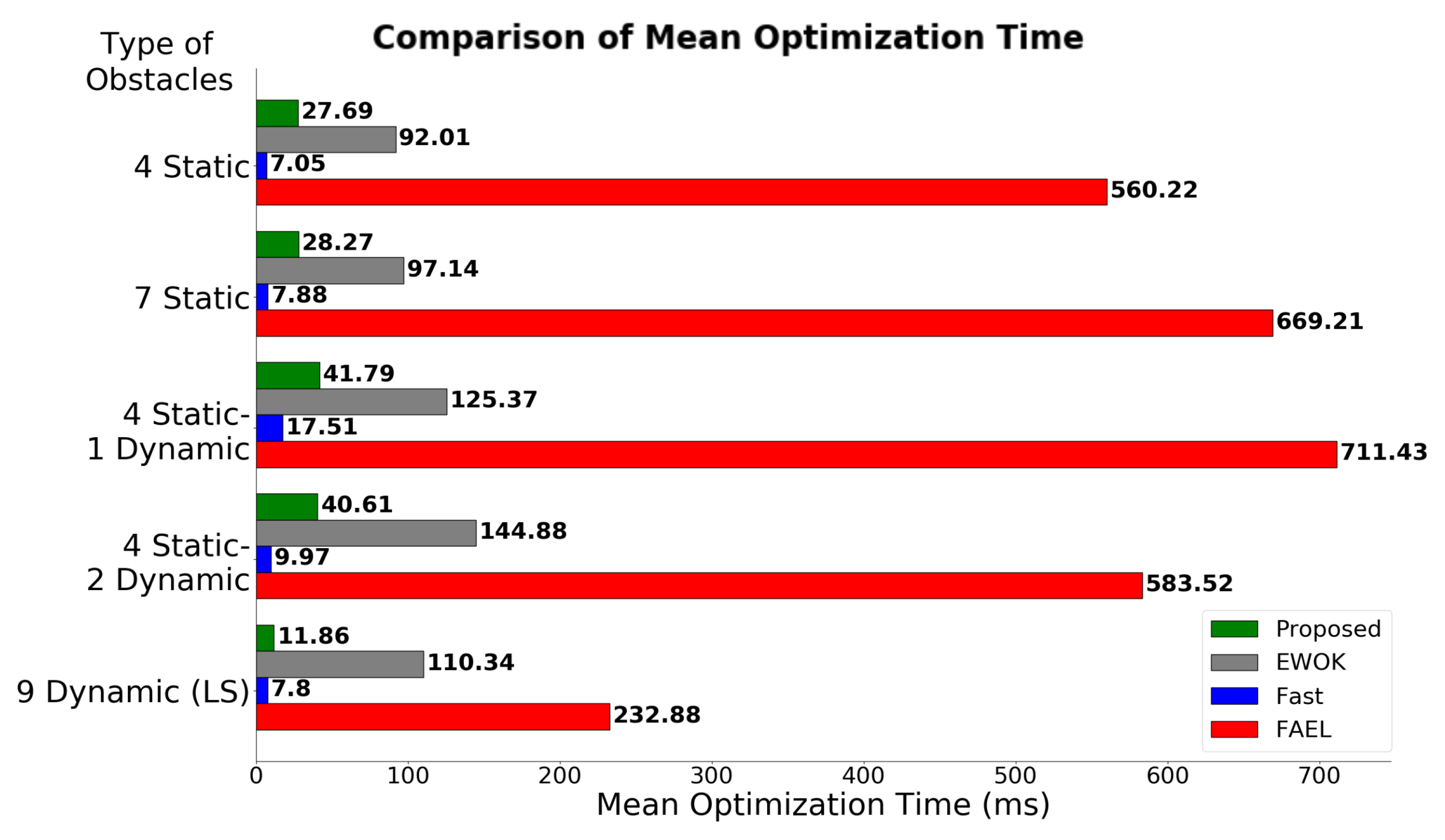
Figure 1. A planning experiment of a mobile robot using only vision-based sensing to localize itself and create an ESDF local map used for optimization-based path replanning. The initial path (pink line) is replanned as presented by the white and green dots based on the obstacles detected in the map (yellow tiles) created by the point cloud.
Robotics 14 00044 g001
Figure 2. An illustration of the variable sized map concept. Three rectangular maps are used to approximate the conical sector shape of the camera-produced point cloud near the lenses. The red and orange boxes at the front of the field-of-view represent a constant-sized part of the generated map, whereas the yellow box represents the part of the map with variable size with respect to the robot’s velocity. Higher linear velocities lead to a map of increased size while reducing the voxel resolution to maintain a high update rate.
Robotics 14 00044 g002
Figure 3. An ESDF map of our experimental setup (top left corner) with a resolution of 0.1 m and a 2 m × 2 m × 1.5 m radius. The yellow tiles represent the occupied voxels over the generated point cloud.
Robotics 14 00044 g003
Figure 4. The rover used for the experimental verification of our algorithms. Marked on the top layer of the electronics box is (a) the onboard computer, (b) the capture card for the camera, (c) the CAN communication module for the motor drives, and (d) DC-DC converters for voltage regulation. The bottom layer (not visible) contains the motor drives and the cooling system.
Robotics 14 00044 g004
Figure 5. (a) The virtual experimental setup with static and dynamic obstacles. (b) The interface of the Scalopus profiler.
Robotics 14 00044 g005
Figure 6. A comparison of mean path planning times for different autonomous navigation approaches in four narrow indoor scenarios and a large-scale scenario with only dynamic obstacles in simulated environments.
Robotics 14 00044 g006
Figure 7. A comparison of mean map update times for different autonomous navigation approaches in four narrow indoor scenarios and a large-scale scenario with only dynamic obstacles in simulated environments.
Robotics 14 00044 g007
Figure 8. Scenarios where the A* approach fails to reach the destination. The red line shows the path for the vehicle following using FAST-Planner, and the blue line shows the path when deploying the proposed approach. (a) Dense obstacles creating narrow corridors. (b) Obstacles forming winding paths with dead ends. (c) Sparse obstacles requiring long detours.
Robotics 14 00044 g008
Figure 9. Real-world autonomous navigation experiment.
Robotics 14 00044 g009
Figure 10. Snapshots of real-world experiments in a dense static environment using the proposed approach (top row) and FAST-Planner (bottom row). (a) The robot is about to avoid the first static obstacle. (b) The robot is at the goal point. (c) The robot is about to avoid the first static obstacle. (d) The robot during a collision with an obstacle.
Robotics 14 00044 g010
Table 1. A comparison of the mean normalized path lengths.
Method4S7S4S-1D4S-2D
Proposed1.1001.1131.2661.153
FAST Planner1.0951.1281.2681.154
Table 2. Success ratio.
MethodNarrowWindingSparse
Proposed0.831.00.8
FAST-Planner0.00.00.0
Disclaimer/Publisher’s Note: The statements, opinions and data contained in all publications are solely those of the individual author(s) and contributor(s) and not of MDPI and/or the editor(s). MDPI and/or the editor(s) disclaim responsibility for any injury to people or property resulting from any ideas, methods, instructions or products referred to in the content.

