Enhancing Positional Accuracy of Mechanically Modified Industrial Robots Using Laser Trackers

Abstract

Highly accurate positioning of industrial robots is crucial to performing industrial operations with high quality. This paper presents a mechanical modification to an industrial robot aiming at enhancing the system actuation resolution, thereby enhancing its positional accuracy. The industrial robot under consideration is a six-degrees of freedom (DoF) robot with revolute joints. By integrating a linear stage, a prismatic joint is introduced to the robot’s end effector, reconfiguring it into a 7 DoF system with more precise step size capabilities. To improve the positional accuracy of the overall system, a closed-loop control structure is chosen. Positional feedback is provided using an industrial laser tracker. Initially, a multi-layer perceptron neural network (MLPNN) is used to identify the forward kinematics (FK) of the overall 6RP robotic system. The FK of the industrial robot using the pretrained MLPNN is then used online to compute the real-time sensitivity of positional error to changes in the joint angle values of the industrial robot and displacements of the prismatic joint. Different trajectories are used to test the accuracy of the proposed positioning algorithm. From the implementation results obtained using the proposed control structure, it is observed that the accuracy of the industrial robot improves significantly. Statistical results for five different points selected from the ISO 9283 trajectory over 30 times of measurements show an 82% improvement for the measurements using the proposed approach as compared to the original industrial robot controller.

1. Introduction

Industrial robots have already gained use in a wide range of applications in areas including object handling [1,2], freeform surface polishing [3], assembly and disassembly [4], machine trending [5], robotic welding [6], painting and coating [7], inspection and quality control [8], packaging and labeling [9], laboratory automation [10], and medical robotics [11]. The primary advantages of deploying industrial robots in these domains are their exceptional dexterity and flexibility and relatively low cost. Ensuring positioning precision is a vital aspect of industrial robot programming that may affect the quality of the given industrial task. For instance, the quality of welding in a marine structure is found to be dependent upon positional accuracy of the industrial robot performing the welding task during the marine structure manufacturing process [6]. Factors such as manufacturing tolerances, parameter measurement, geometrical uncertainties, and low stiffness of the robot joints result in inaccuracy in the robot positioning. Consequently, there is a need to enhance the accuracy of industrial robots during operations through the application of advanced measurement techniques.

To enhance the positional accuracy of industrial robots, both offline and online methods have been examined [12]. Increasing the accuracy of Denavit–Hartenberg (DH) parameters of industrial robots including link lengths, link offsets, joint twists, and initial values of joint angle values constructs a major class of characterization approaches [13]. Most of the techniques for increasing the accuracies of industrial robot DH parameters are offline methods. However, offline characterization approaches can only deal with kinematics errors within an industrial robot. Non-kinematics factors may result in positioning errors during robot operations [12]. Flexibilities within robot structure, thermomechanical effects [14,15], link inertia, backlash [15], non-uniform mass distributions within links [16], loads, and self-weights of industrial robot effects may result in non-kinematic errors [12]. Under load and vibration conditions, low stiffness within robot joints may result in deflection, which cannot be compensated offline. Therefore, it is required to compensate for non-kinematic factors using real-time control systems [17]. Online approaches, on the other hand, perform closed-loop control of industrial robot position, which may lead to more accurate control of the industrial robot. The use of artificially intelligent approaches, such as artificial neural networks (ANNs), to compensate for positional inaccuracy in a non-parametric methodology online is a major class of online approaches in the literature. Examples of such approaches are the ones that use different laser tracker systems for precision positioning tasks for robot arms such as PA10 robot arm and IRB1410 [18,19,20]. Similarly, non-parametric calibration for Hyundai HH800 industrial robot using laser tracker is investigated [18,21]. While moving heavy objects, vibrations may occur within a robotic structure, and to suppress such vibrations, a heuristic approach is investigated in [17]. Pose error compensation for an industrial robot using gradient descent of its forward kinematics is investigated in [22] where a laser tracker is used to measure the position of a heavy duty industrial robot. Machine vision using Aruco markers as another position measurement method has been investigated in [23] for characterization purposes of an industrial robot. However, the precision obtained using Aruco markers as the measurement equipment for pose measurement is far below the precisions that can be obtained using laser tracker for pose measurement. In [24], ANNs have been used to develop a model for the effect of non-kinematic sources of positional uncertainty including geometric errors, joint deflection errors, and non-geometrical errors. Similarly, a deep belief neural network optimized by differential evolution is utilized in [25] for an absolute position compensation system for an industrial robot. The use of an error compensation scheme in parallel with the theoretical model of an industrial robot is another method to utilize the geometrical knowledge about the industrial robot [16]. The error compensation approach based on incremental support vector machine, in this case, is not the sole inverse kinematics solver for the system, but rather it compensates for the theoretical model errors. In summary, although many offline and online approaches exist in the literature to characterize industrial robots for superior positioning performance, the resolution of motion in industrial robots is limited by their joint angle measurement resolution. Therefore, the current paper addresses mechanical modification to an industrial robot to increase its positional resolution.

In this paper, mechanical modifications along with implementations of advanced positional algorithms are proposed to enhance the positional accuracy of an industrial robot. The industrial robot considered in this paper is a serial manipulator that benefits from six revolute joints. The resolution of the linear motion in this industrial robot is limited by the accuracy of the joint angle measurements and its joint angle controller. The main contributions of the paper are highlighted as follows:

• Integrating a more accurate linear move stage as an active end effector for the industrial robot to enhance its motion resolution;
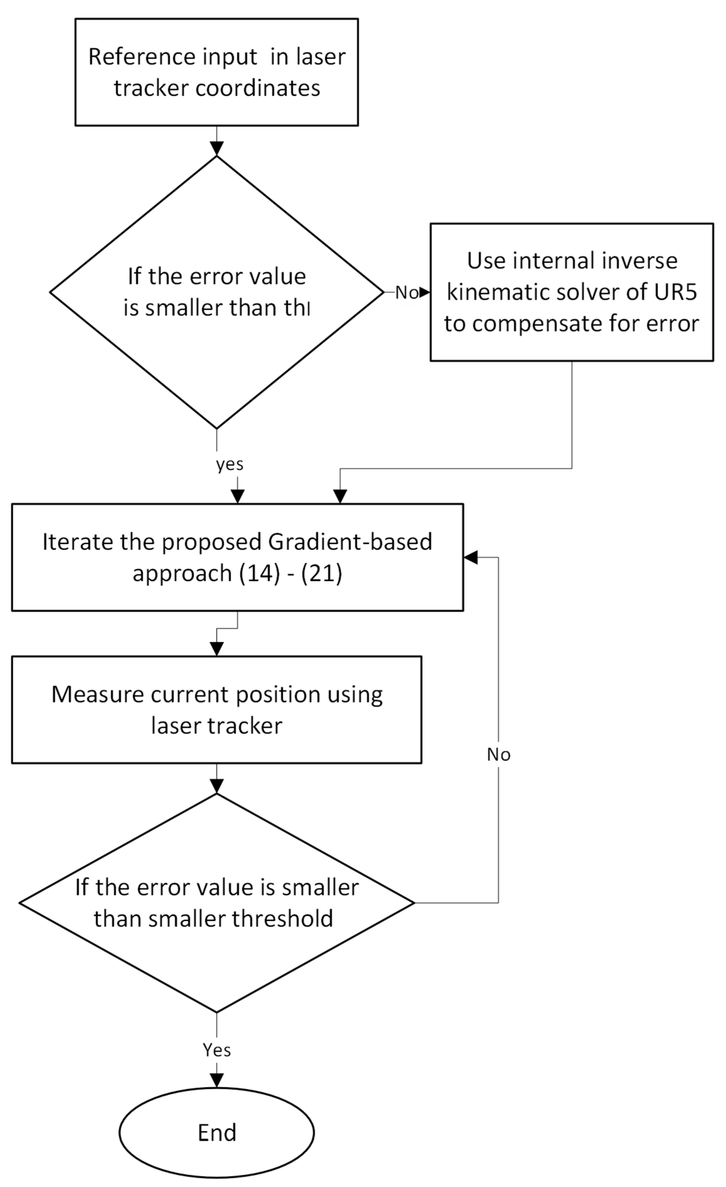
• Employing gradient descent to tune the industrial robot joint angle values and displacement of the linear move stage by using the identified forward kinematics (FK) of the overall system for the calculation of the required partial derivates of the actual position of the end effector with respect to DH parameters of the overall system.

The first contribution of the current paper is the enhancement of motion resolution in industrial robots through the integration of a linear move stage with enhanced accuracy at the end effector. This addition increases the degrees of freedom of the industrial robot by incorporating a prismatic joint, thereby transferring the overall system into a 6RP robotic system. The name 6RP robot is a naming convention for robots widely known in the robotic community, which refers to a robot with six revolute joints and a prismatic joint. To compensate for non-kinematics errors, real-time and closed-loop joint angle control of a modified industrial robot is proposed. Positional feedback is provided from the system using a highly accurate industrial laser tracker system. The FK of the overall mechanically modified system is identified using an artificial neural network. This FK model is subsequently employed within real-time control of the mechanically modified system to estimate the gradient of the real-time industrial robot position error with respect to joint angle values of the industrial robot and linear displacement of the linear move stage. Consequently, the industrial robot joint angle values and the linear displacement of the linear move stage are adaptively adjusted online. Using this approach, it is shown that the position performance of the overall augmented system increases considerably. Furthermore, the performance of the proposed algorithm in tracking a selection of points out of an ISO 9283 [26,27] trajectory is investigated. It is observed that using the proposed approach, it is possible to increase the positional accuracies of the industrial robot for all investigated trajectories for at least 82%.

The rest of this paper is organized as follows: In Section 2, the methodology implemented in this paper is given. The system setup including the industrial robot, linear move stage, and the laser tracker is given in Section 3. The results are given in Section 4, which are followed by the conclusion in Section 5, acknowledgements in the back matter. The references are provided at the end of the paper.

2. Methodology

2.1. Forward Kinematics

The geometrical forward kinematics (FK) of the industrial robot using Denavit–Hartenberg (DH) parameters identifies its Cartesian position. The DH parameters of an industrial robot are link length, link offset, link twist, and joint angle. Similar to most 6RP industrial robots, only joint angle values are controlled during robot operation within UR5. UR5 is the name of the robot manufactured by Universal Robot that is investigated in this paper. This industrial robot complies with ISO 10218-1 and -2 [28,29] (https://www.universal-robots.com/articles/ur/safety/safety-faq/). The overall FK of UR5 is calculated as the product of link transformations.

$$T_e={}_6{}^{0}T={}_1{}^{0}T{}_2{}^{1}T{}_3{}^{2}T{}_4{}^{3}T{}_5{}^{4}T{}_6{}^{5}T,$$

(1)

where ${}_i{}^{i-1}T$ is the link transformation matrix for link $i$ [30,31].

$${}_i{}^{i-1}T=\left[\begin{array}{cccc}{cq}_i& -{c{\alpha }_{i}sq}_i& {s{\alpha }_{i}sq}_i& {a_{i}cq}_i\\ {sq}_i& c{\alpha }_i{cq}_i& -s{\alpha }_i{cq}_i& {a_{i}sq}_i\\ 0& s{\alpha }_i& c{\alpha }_i& d_i\\ 0& 0& 0& 1\end{array}\right],$$

(2)

where $q_i’s,i=1,\dots ,6$ represent the joint angle $i$, ${\alpha }_i’s,i=1,\dots ,6$ represent link twist, $a_i’s,i=1,\dots ,6$ represent link length, and $d_i’s,i=1,\dots ,6$ represent link offset. These areother DH parameters of the industrial robot. Furthermore, ${cq}_i,{sq}_i,c{\alpha }_i,\mathrm{a}\mathrm{n}\mathrm{d}s{\alpha }_i,i=1,...6$ represent ${cos(q}_i),$ ${sin(q}_i),$ $c{os\alpha }_i,$ and $sin\left({\alpha }_i\right),i=1,...,6$, respectively. The DH parameters of UR5 are given in

Table 1. The DH parameters of the 6 DoF robot positional error.

Link	$\mathit{q}$	$\mathit{d}$	$\mathit{a}$	$\mathit{\alpha }$
1	$q_1$	$d_1$	0	$\pi /2$
2	$q_2$	0	$a_2$	0
3	$q_3$	0	$a_3$	0
4	$q_4$	$d_4$	0	$\pi /2$
5	$q_5$	$d_5$	0	$-\pi /2$
6	$q_6$	$d_6$	0	0

.

2.2. Computational Forward Kinematics Identification of the Overall System

ANNs imitate biological neurons and their signal exchange to provide a nonlinear map between their input and output. In the case when a nonlinear function is unknown, ANNs are among the preferred choices for function approximation as they can approximate a large class of nonlinear functions, and they benefit from a systematic structure for this purpose. Their structure can easily be expanded in terms of the number of neurons and hidden layers to increase general function capability to gain better fitting performance. It is further possible to extend identification capability of the ANN to a larger area using an ANN with a higher number of neurons and number of layers. To find the position of the overall robotic system that includes an industrial robot and a linear move stage, its computational FK is required. There exist some uncertainties in the industrial robot FK and the mountings used to attach the move stage to the industrial robot and within the move stage. Therefore, to identify the computational FK of this system, a multi-layer perceptron neural network (MLPNN) structure is preferred. To train this structure, joint angle values of the industrial robot and displacement of the move stage are taken as input values, and actual position of the end effector measured by the laser tracker is taken as the target value. The input taken for the MLPNN in this study is ${\left[\begin{array}{cc}\begin{array}{cc}{q}_1& \dots \end{array}& \begin{array}{cc}{q}_6& x_m\end{array}\end{array}\right]}^T$, where $x_m$ is the linear displacement of the linear move stage. The number of hidden layer neurons for this structure is taken as equal to 10. The training approach for this structure is Levenberg–Marquardt algorithm. The target values for the MLPNN are taken as ${\left[\begin{array}{ccc}{x}_L& y_L& z_L\end{array}\right]}^T$ where $x_L,y_L,$ and $z_L$ are the position of the overall 6RP end effector in the 3D space measured by the laser tracker system. To measure the 3D position, a laser target is mounted on the move stage.

Assuming L is the total number of layers in the MLPNN and $l_i,i=1,\dots ,L$ is the total number of neurons in each layer, $o_i\in R^{l_i},i=0,\dots ,L$ is the output of each layer, and $f_i(.),i=1,\dots ,L$ is the activation function for each layer, we have the following equation for each layer in the MLPNN (see Figure 1):

$$o_i=f_i(W_i{o}_{i-1}+b_i),$$

(3)

where $W_i\in R^{l_i\times l_{i-1}}$ are the weights of the MLPNN, and $b_i\in R^{l_i}$ are the bias terms in the MLPNN. It is to be noted that $o_0$ is the input vector for the MLPNN.

$${o_0=\left[\begin{array}{cc}\begin{array}{cc}{q}_1& \dots \end{array}& \begin{array}{cc}{q}_6& x_m\end{array}\end{array}\right]}^T\in R^7,$$

(4)

The activation function, $f_1$, for the single hidden layer considered in this paper is a bipolar sigmoid function and for the output layer, $f_2$, is a linear activation function:

$$\begin{gathered} f_1\left(r\right)=\mathrm{tansig}\left(r\right)={\displaystyle \frac{2}{\exp \left(-2r\right)+1}}-1, \\ {f}_2\left(r\right)=\mathrm{lin}\left(r\right)=r \end{gathered}$$

(5)

The cost function $J$ is defined as the sum of squares of the current error value of the MLPNN in all dimensions:

$$J={{\displaystyle \frac{1}{2}}(T-o_L)}^T(T-o_L),$$

(6)

where

$${D=\left[\begin{array}{ccc}{x}_L& y_L& z_L\end{array}\right]}^T,$$

(7)

is the target vector for MLPNN measured by the laser tracker. The partial derivate of the cost function $J$ with respect to the MLPNN parameters is obtained as follows:

$${\displaystyle \frac{\partial J}{W_i}}=S_i{o}_{i-1}^T,{\displaystyle \frac{\partial J}{b_i}}=S_i,$$

(8)

where $S_i$ is obtained as follows:

$$S_i={\dot{F}}_i\left({W_i^{T}o}_{i-1}+b_i\right)W_{i+1}^T{S}_{i+1},i=1,\dots ,L-1,$$

(9)

where

$${\dot{F}}_i\left(o_i\right)=\left[\begin{array}{cccc}{\dot{f}}_i\left(o_{i,1}\right)& 0& \cdots & 0\\ 0& {\dot{f}}_i\left(o_{i,2}\right)& \ddots & ⋮\\ ⋮& \ddots & \ddots & 0\\ 0& \cdots & 0& {\dot{f}}_i\left(o_{i,l_i}\right)\end{array}\right],$$

(10)

is the matrix whose diagonal elements are the derivative values of the activation function $f_i$ with respect to the elements of $o_i$. While ${\dot{f}}_i(.)$ for a linear activation function is equal to 1, for a bipolar sigmoid activation function, we have

$${\dot{f}}_i\left(u\right)=1-u^2,$$

(11)

Finally, $S_L$is obtained as follows:

$$S_L=-2{\dot{F}}_L\left({W_L^{T}o}_{L-1}+b_L\right)\left(D-o_L\right),$$

(12)

The Levenberg–Marquardt algorithm is used to train MLPNN for $W_i,b_i,i=1,\dots ,L$.

2.3. Computational Sensitivity Analysis of the Industrial Robot FK

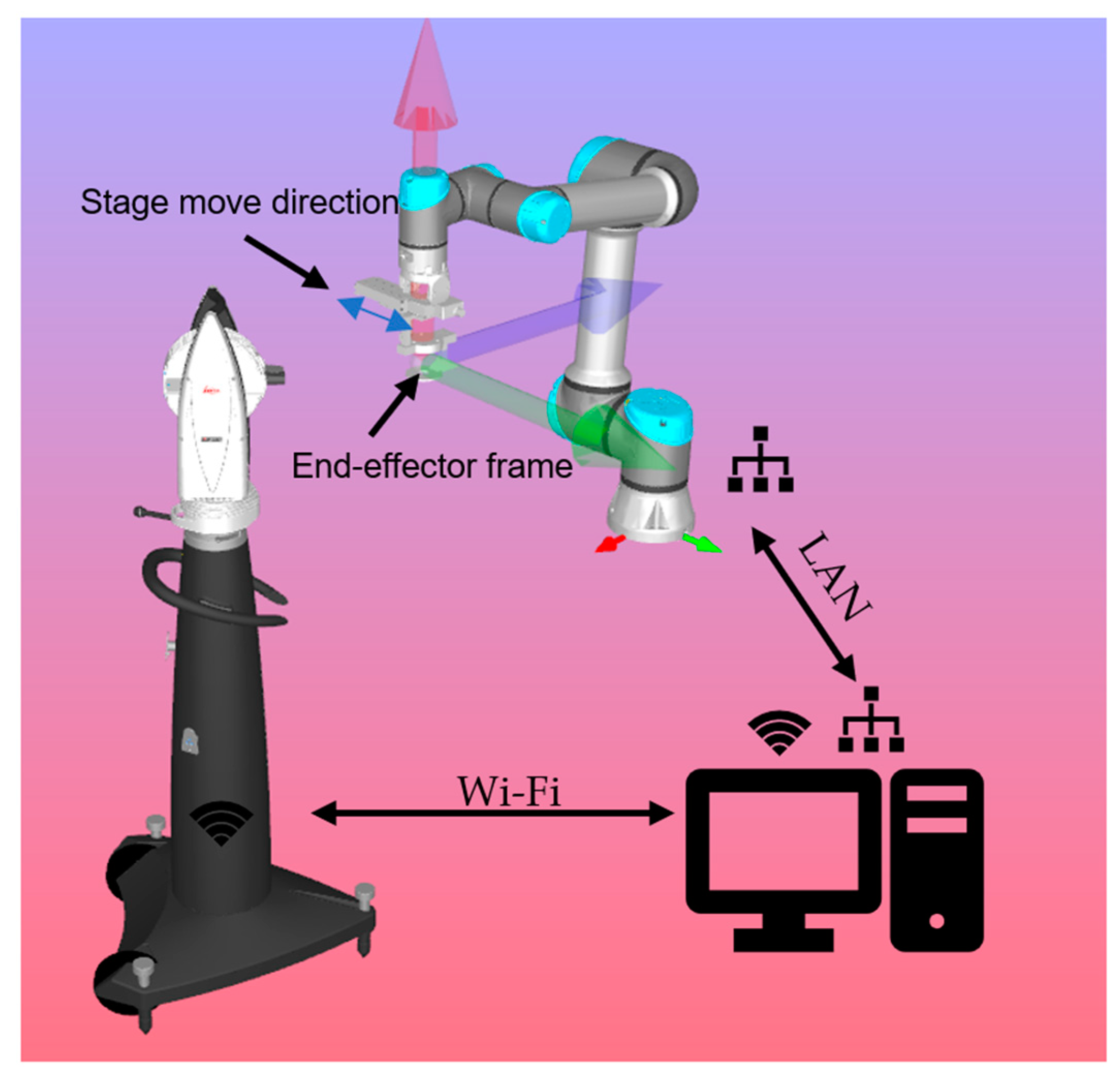
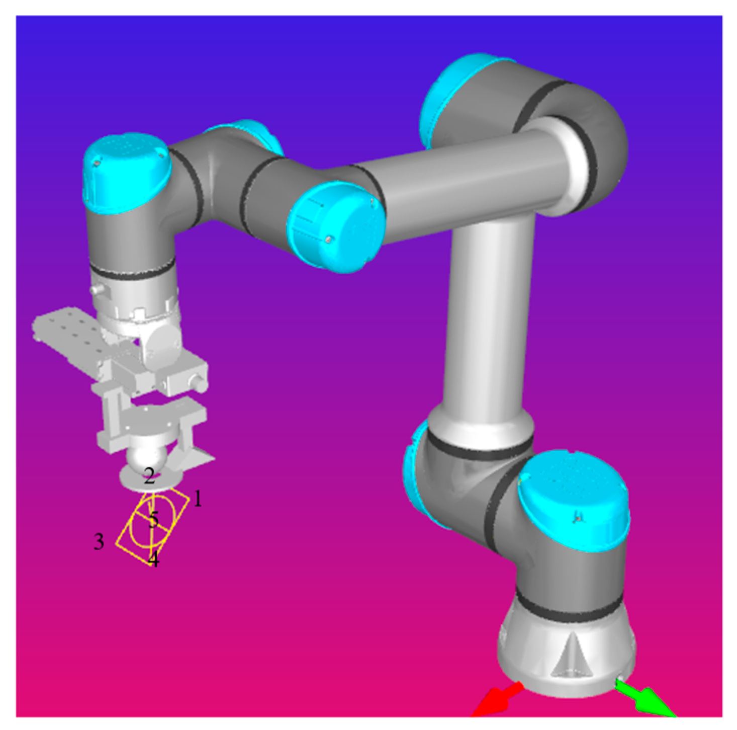
To position the overall 6RP industrial robot, at first step, a large threshold value ${th}_l$ is selected. Positional errors larger than this value are compensated by using a movement in the industrial robot to compensate for these error values. A coordinate change may be required because of the difference in the coordinate system of the industrial robot and the laser tracker system as follows:

$${{}_{L}T}_e={}_L{}^{R}T{T}_e,$$

(13)

where ${{}_{L}T}_e$ is the transformation matrix of the industrial robot in laser tracker coordinates, and ${}_L{}^{R}T$ is the matrix that performs the coordinate change.

A few iterations may be required to compensate for the errors larger than ${th}_l$. When positional error is less than ${th}_l$, gradient descent-based optimization algorithm is utilized to compensate for smaller positional error values. Gradient descent algorithm is a frequently used optimization algorithm for nonlinear function optimization tasks. This optimization technique requires the partial derivative of the cost function with respect to the adaptable parameters. The MLPNN developed in the previous subsection is, therefore, used to calculate the partial derivative function. In the first step, the MLPNN is trained over a gathered dataset. The trained MLPNN is then used in an online setting to find correction terms for the parameters of the overall 6RP robot including joint angle values and linear displacements.

Partial derivatives of the outputs of the MLPNN to its inputs are obtained as follows:

$$S_{O_0}={\displaystyle \frac{\partial o_2}{\partial o_0}}={\displaystyle \frac{\partial o_2}{\partial o_1}}{\displaystyle \frac{\partial o_1}{\partial o_0}},$$

(14)

where

$$\begin{gathered} {\displaystyle \frac{\partial o_2}{\partial o_1}}={\dot{F}}_2\left({W_2^{T}o}_1+b_2\right)W_2^T \\ {\displaystyle \frac{\partial o_2}{\partial o_1}}={\dot{F}}_1\left({W_1^{T}o}_0+b_1\right)W_1^T, \end{gathered}$$

(15)

Therefore, partial derivatives of the MLPNN for 6RP parameters are obtained as the elements of $S_{O_0}$, such that

$$S_{O_0}={\left[\begin{array}{cc}\begin{array}{cc}{S}_{q_1}& \dots \end{array}& \begin{array}{cc}{S}_{q_6}& S_{x_m}\end{array}\end{array}\right]}^T,$$

(16)

The joint angle values of the industrial robot and positional displacement of the linear stage iterate for a few iterations until positional error value is less than ${th}_s$. The flowchart of this experiment is given in Figure 2.

To compensate for the positional error for the industrial robot end effector, gradient descent approach is utilized. The gradient descent approach used in this paper relies on the partial derivative computed through the MLPNN developed in the previous subsection. The transformation matrix of the industrial robot end effector in the laser tracker coordinate is given as follows [32]:

$$\begin{gathered} {{}_L{}^{}T}_e={{}_L{}^{}T}_e\left(x_D+∆x_D,y_D+∆y_D,z_D+∆z_D\right)R\left(x_D,{\theta }_{x_D}+∆{\theta }_{x_D}\right) \\ R(y_D,{\theta }_{y_D}+∆{\theta }_{y_D})R(z_D,{\theta }_{z_D}+∆{\theta }_{z_D}) \end{gathered}$$

(17)

where $\left(\begin{array}{ccc}{x}_D,& y_D,& z_D\end{array}\right)$ are the desired end-effector coordinates in 3D space, $\left(\begin{array}{ccc}{\theta }_{x_D},& {\theta }_{y_D},& {\theta }_{z_D}\end{array}\right)$ are the desired end-effector orientations in 3D space, $∆x_D$, $∆y_D$, and $∆z_D$ are the deviations of the current end-effector values from their desired values, and $∆{\theta }_{x_D}$, $∆{\theta }_{y_D}$, and $∆{\theta }_{z_D}$ are the deviations of the industrial robot end-effector rotations from the desired value.

$$\left(\begin{array}{c}{∆x}_D\\ {∆y}_D\\ {∆z}_D\end{array}\right)=\left(\begin{array}{c}{{}_L{}^{}T}_{e\left(\mathrm{1,4}\right)}\left(q+∆q\right)-{{}_L{}^{}T}_{e\left(\mathrm{1,4}\right)}\left(q\right)\\ {{}_L{}^{}T}_{e\left(\mathrm{2,4}\right)}\left(q+∆q\right)-{{}_L{}^{}T}_{e\left(\mathrm{2,4}\right)}\left(q\right)\\ {{}_L{}^{}T}_{e\left(\mathrm{3,4}\right)}\left(q+∆q\right)-{{}_L{}^{}T}_{e\left(\mathrm{3,4}\right)}\left(q\right)\end{array}\right)$$

(18)

where ${{}_L{}^{}T}_{e\left(i,j\right)}\left(q+∆q\right)$ is the element of the matrix ${{}_L{}^{}T}_e$ in the i-th row and j-th column. The following relationship holds for the deviations of the end-effector positions and the changes in the industrial robot joint angle values.

$$\left(\begin{array}{c}{∆x}_D\\ {∆y}_D\\ {∆z}_D\end{array}\right)=\left(\begin{array}{c}\begin{array}{cc}\begin{array}{cc}{\displaystyle \frac{{\partial {}_L{}^{}T}_{e\left(\mathrm{1,4}\right)}}{{\partial q}_1}}& {\displaystyle \frac{{\partial {}_L{}^{}T}_{e\left(\mathrm{1,4}\right)}}{{\partial q}_2}}\end{array}& \begin{array}{cc}\cdots & \begin{array}{cc}{\displaystyle \frac{{\partial {}_L{}^{}T}_{e\left(\mathrm{1,4}\right)}}{{\partial q}_6}}& {\displaystyle \frac{{\partial {}_L{}^{}T}_{e\left(\mathrm{1,4}\right)}}{{\partial x}_m}}\end{array}\end{array}\end{array}\\ \begin{array}{cc}\begin{array}{cc}{\displaystyle \frac{{\partial {}_L{}^{}T}_{e\left(\mathrm{2,4}\right)}}{{\partial q}_1}}& {\displaystyle \frac{{\partial {}_L{}^{}T}_{e\left(\mathrm{2,4}\right)}}{{\partial q}_2}}\end{array}& \begin{array}{cc}\cdots & \begin{array}{cc}{\displaystyle \frac{{\partial {}_L{}^{}T}_{e\left(\mathrm{2,4}\right)}}{{\partial q}_6}}& {\displaystyle \frac{{\partial {}_L{}^{}T}_{e\left(\mathrm{2,4}\right)}}{{\partial x}_m}}\end{array}\end{array}\end{array}\\ \begin{array}{cc}\begin{array}{cc}{\displaystyle \frac{{\partial {}_L{}^{}T}_{e\left(\mathrm{3,4}\right)}}{{\partial q}_1}}& {\displaystyle \frac{{\partial {}_L{}^{}T}_{e\left(\mathrm{3,4}\right)}}{{\partial q}_2}}\end{array}& \begin{array}{cc}\cdots & \begin{array}{cc}{\displaystyle \frac{{\partial {}_L{}^{}T}_{e\left(\mathrm{3,4}\right)}}{{\partial q}_6}}& {\displaystyle \frac{{\partial {}_L{}^{}T}_{e\left(\mathrm{3,4}\right)}}{{\partial x}_m}}\end{array}\end{array}\end{array}\end{array}\right)\left(\begin{array}{c}\begin{array}{c}{∆q}_1\\ {∆q}_2\end{array}\\ \begin{array}{c}⋮\\ \begin{array}{c}{∆q}_6\\ {∆x}_m\end{array}\end{array}\end{array}\right)$$

(19)

Using the relationship given in (19), the following update rule for the joint angle values of the industrial robot and the displacement of the move stage is used to compensate for the position error and correct the joint angle values and the displacement to increase the accuracy of the industrial robot:

$$\begin{gathered} {∆q}_i={\gamma }_i{\displaystyle \frac{{\partial {}_L{}^{}T}_{e\left(\mathrm{1,4}\right)}}{{\partial q}_i}}{∆x}_D+{\gamma }_i{\displaystyle \frac{{\partial {}_L{}^{}T}_{e\left(\mathrm{2,4}\right)}}{{\partial q}_i}}{∆\mathrm{y}}_D+{\gamma }_i{\displaystyle \frac{{\partial {}_L{}^{}T}_{e\left(\mathrm{3,4}\right)}}{{\partial q}_i}}{∆z}_D,{\gamma }_i>0,i=1\dots ,6 \\ {∆x}_m={\gamma }_m{\displaystyle \frac{{\partial {}_L{}^{}T}_{e\left(\mathrm{1,4}\right)}}{{\partial x}_m}}{∆x}_D+{\gamma }_m{\displaystyle \frac{{\partial {}_L{}^{}T}_{e\left(\mathrm{2,4}\right)}}{{\partial x}_m}}{∆y}_D+{\gamma }_m{\displaystyle \frac{{\partial {}_L{}^{}T}_{e\left(\mathrm{3,4}\right)}}{{\partial x}_m}}{∆\mathrm{z}}_D,{\gamma }_m>0 \end{gathered}$$

(20)

where the following values are obtained using the trained MLPNN:

$$\begin{gathered} {\displaystyle \frac{{\partial {}_L{}^{}T}_{e\left(j,4\right)}}{{\partial q}_i}}={\displaystyle \frac{{\partial {}_L{}^{}T}_{e\left(j,4\right)}}{{\partial x}_L}}{\displaystyle \frac{{\partial x}_L}{{\partial q}_i}},j=1,\dots ,3,i=1,\dots ,6 \\ {\displaystyle \frac{{\partial {}_L{}^{}T}_{e\left(j,4\right)}}{{\partial x}_m}}={\displaystyle \frac{{\partial {}_L{}^{}T}_{e\left(j,4\right)}}{{\partial x}_L}}{\displaystyle \frac{{\partial x}_L}{{\partial x}_m}},j=1,\dots ,3,i=1,\dots ,6 \end{gathered}$$

(21)

3. System Setup

The overall experimental setup consists of a UR5 with a linear stage mounted on its end effector to provide a 6RP industrial robot. A laser target is mounted on the linear stage where the 3D position of the end effector is measured by a laser tracker. This experimental setup is depicted in Figure 3. Each of the individual components to perform the experiment are explained in detail in this section.

3.1. Industrial Robot

The Universal Robot—UR5—is a serial manipulator with six revolute joints with rated maximum load capacity of 5 kg. UR5 consists of three main components including the manipulator, robot controller, and teaching pendant. The maximum angular velocity of this industrial robot on each of its joints are $180°/\mathrm{s}$, and its maximum angular acceleration is $180°/{\mathrm{s}}^2$. Its joints can rotate up to $\pm 360°$, and it can span a sphere of 850 mm around it except for its singular points within the sphere including the cylinder on top of the base and some orientations close to the border of the sphere. The robot benefits from LAN connectivity that makes it controllable directly from a PC using its API within Python. There is community support for UR5 through Universal Robots that provides support for its Python API. The Python API features some functionality such as joint angle readings, 3D position readings, and transformation matrix readings from the robot. It further makes it possible to control the UR5 through control functions that are embedded within the robot controller including MoveJ, MoveL, MoveP, and MoveC commands [33]. This minimizes the necessity for writing code for point-to-point motion for the robot.

MoveJ command is a joint-based command that controls the robot between its waypoints by changing joint angle values to the desired ones to hit the target waypoint. In this type of motion, all joints move towards their desired values independently. No special trajectory is fulfilled during the robot operation in this mode. Maximum angular and linear values for the robot speed and maximum values for angular and linear robot accelerations can be set during operation.

MoveP adds an extra feature to the MoveL command by controlling the linear speed value for the robot to maintain a constant value during its motion.

MoveC defines a circular motion between the start point and end point through an auxiliary point between the two points.

The use of Python API makes it possible to directly utilize the commands given through the robot controller, which saves programming time and will result in a reliable method for positioning the industrial robot. However, this method suffers from errors, as within an industrial robot, no feedback is provided from the actual industrial robot end effector.

3.2. Linear Move Stage

Joint clearance error is among factors that influence the industrial robot positional accuracy [34]. The actual rotational error in UR5 joint angle encoders is 0.1° [35], which introduces limitations to the accurate positioning of its end effector. To increase the controllability of this industrial robot, a high-precision linear move stage is added to its end effector. This linear stage can work independently in a wide range of applications including marine applications [36], aviation industry, and 3D printing [37,38]. In this paper, this stage is added to the industrial robot to increase its motion resolution and provide its fine-tuning capability. The technical specifications of this robot include load capacity of 250 N, maximum displacement of 5 cm, and motor current rating of 600 mA/phase. According to the manufacturer, its accuracy is up to 8 µm and its resolution is 50 nm. However, the maximum load capacity of the overall industrial robot and linear stage is limited by the load capacity of the industrial robot minus the weight of the linear stage and its fixtures. The connectivity of this motion stage with PC is provided using a built-in RS232/USB converter with baud rate of 115.2 Kbps. Communication with this equipment is provided through Python 3 API provided by the manufacturer (https://www.zaber.com/software visited: 22 March 2025).

The linear stages are connected to the PC in a Daisy chain network connection. Therefore, in the case of multiple Zaber linear stages connected to a PC, it is required to identify all stages within the Python command. For moving to a linear stage, two modes of operations, namely absolute motion and relative motion, are available. The unit for motions is identified within the motion commands.

3.3. Laser Tracker System

To provide precision measurement to identify overall FK of the system, a laser tracker is utilized. The laser tracker used in this experiment is AT960-MR which is manufactured by Hexagon Metrology Limited, UK. To perform measurement, it uses a single class II laser source that hits a retroreflective target. The laser tracker identifies two angles and the distance to the retroreflective target. The distance is measured by measuring the phase shift between the emitted light and the reflected light from the 1.5″ red ring reflector. The principles of corner cube are used in the structure of the retroreflector. Three perpendicular mirrors are used in the structure of the retroreflector to make laser light hit the center of the target, and this point is always the measured point during the experiments. The laser tracker equipment is designed to have an ingress protection against dust and other contaminants. One of the limitations of using a laser tracker to measure position, which may limit its operation, is line of sight between the laser tracker and the laser target. In the case of an object blocking the line of sight between the laser tracker and the laser target, or the laser target not being aligned with the laser tracker, measurement would be disturbed. Therefore, within the experiment, it is required to make sure that no object including robot arms blocks the line of sight between the laser tracker and the laser target. Another limitation for the laser tracker with a single target is that it provides position measurement in 3D, and the orientation of the end effector cannot be measured using this equipment. The connectivity to this equipment is provided through Wi-Fi connectivity.

3.4. Overall Connectivity

Robot joint angle values and the displacement within the linear stage are recorded using their connectivity with PC through their Python API. The position values of the end effector are recorded using the laser tracker that are transferred to the same PC using its Wi-Fi connectivity. These position values are analyzed using Spatial Analyzer software version 2019.05.16 and are published using user datagram protocol (UDP). UDP is available within MATLAB R2024 and provides the position measurements to the same Python script to avoid synchronization issues. This connection diagram is depicted in Figure 4. The end-effector frame as well as the move stage movement direction are also depicted in this figure.

3.5. Uncertainty Analysis of the Overall System

The industrial robot used in this experiment and the linear stage added to its end effector benefit from high levels of accuracy, which make it possible to use them in a feedback loop to increase the overall positional accuracy. However, when the industrial robot is equipped with a move stage, its geometry totally changes. The overall uncertainty analysis for the 6RP system has been previously performed in [35]. Because of the nonlinear nature of the FK of the two systems, uncertainty analysis for the 6RP robot depends on the joint angle values of the industrial robot and the position of the linear stage. Therefore, statistical analysis for the positioning of the overall system is performed for a few points in [35]. The interested reader is referred to that paper for further uncertainty analysis of the 6RP system.

4. Results

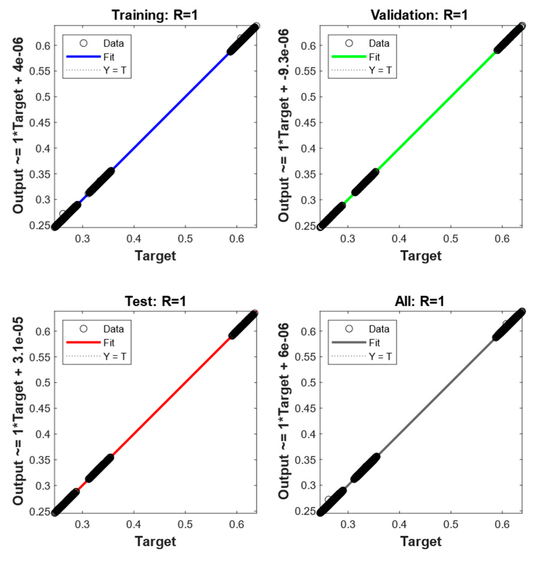
4.1. MLPNN Forward Kinematics Identification of the Overall System

The performance of the MLPNN for FK identification of the overall 6RP industrial robot is presented in this section. An MLPNN benefits from a single hidden layer with 10 neurons in this layer, input signal of ${\left[\begin{array}{cc}\begin{array}{cc}{q}_1& \dots \end{array}& \begin{array}{cc}{q}_6& x_m\end{array}\end{array}\right]}^T$, and target signal of ${\left[\begin{array}{ccc}{x}_L& y_L& z_L\end{array}\right]}^T$. A few trials and errors are performed to select the best MLPNN structure, and finally the number of neurons in the hidden layer is selected as equal to 10. The training method used for this identification process is the Levenberg–Marquardt algorithm. The overall training procedure for this training algorithm given in Figure 5 demonstrates convergence of the training method after 19 epochs. The test RMSE value for the test process is obtained as equal to $1.35\times {10}^{-4}\mathrm{m}$. The results of R² test in these experiments are given in Figure 6. The results of R² are satisfactory as the coefficient value for this training procedure is one and the bias term is a very small value. Therefore, FK of the industrial robot has been identified with high performance. To have a visual comparison between target data and MLPNN output values, Figure 7 is presented. As can be seen from these figures, MLPNN output closely follows industrial robot FK target values in all three dimensions.

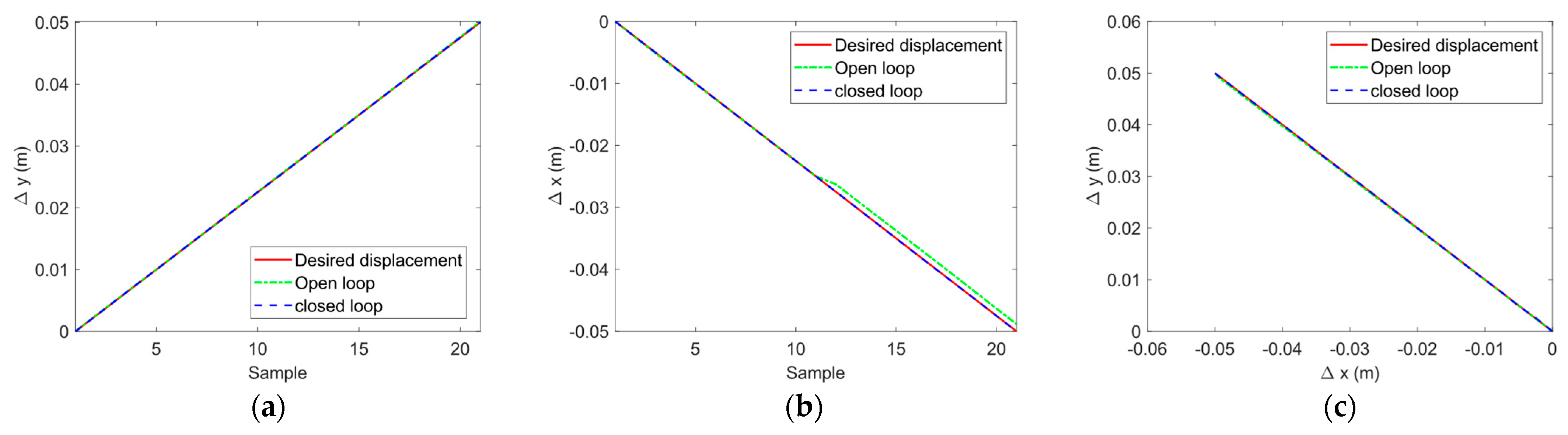
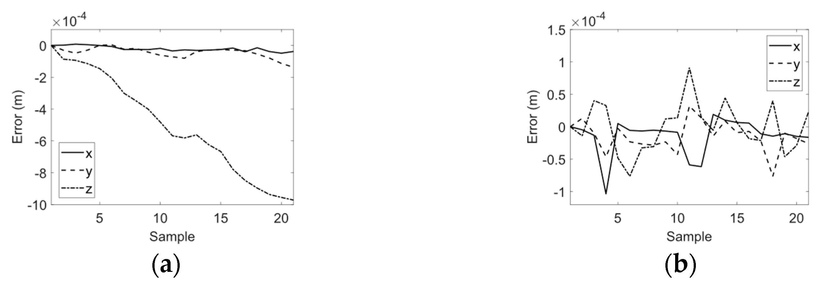
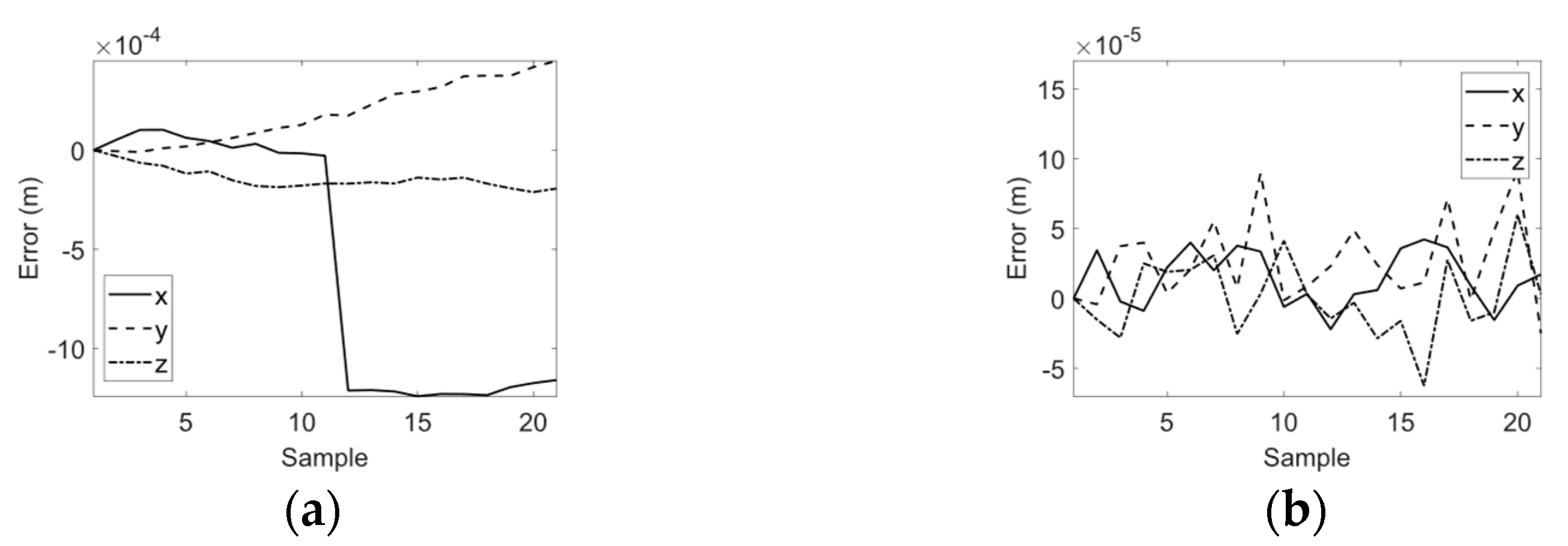
4.2. Precision Positioning of the Robot

To test the accuracy of the proposed positioning algorithm on an industrial robot in real time, three different experiments are designed. In the first experiment, the following trajectory is considered for the robot:

$$∆x_i=0,∆y_i=2.5\times (i-1)mm,{∆z}_i=0,i=1,...,21$$

where $∆x_i,∆y_i,$ and ${∆z}_i$ are the displacement commands from the home position in each of the axes for the ith sample (see Figure 8a). The home positions in robot coordinates for the three experiments are equal and are taken as follows:

$$\begin{gathered} x_0=0.4621,y_0=-0.1080,x_0=0.2700, \\ {r}_x=2.102,r_y=-2.348,r_z=0.0, \end{gathered}$$

where $x_0,y_0,$ and $z_0$ are coordinates of the initial point in the three dimensions, and $r_x,r_y,$ and $r_z$ are rotations about the three axes. In the second experiment, the following trajectory is considered for the robot (see Figure 8b):

$$∆x_i=-2.5\times (i-1)mm,∆y_i=0,{∆z}_i=0,i=1,...,21$$

Finally, in the third experiment, the following trajectory is considered for the robot (see Figure 8c):

$$∆x_i=-2.5\times (i-1)mm,∆y_i=2.5\times (i-1)mm,{∆z}_i=0,i=1,...,21$$

The overall trajectory tracking for the robot in the three dimensions for the three experiments is given in Figure 8. The movements between the points are performed using relative motion using the MoveL command through Python urx version 0.11.0 software package. The error values for the three experiments are for the open-loop and the closed-loop robot operations using the proposed algorithm and are given in Figure 9, Figure 10 and Figure 11, respectively. From these figures, it is observed that the proposed robot positioning algorithm is capable of controlling the position of the robot with higher accuracy as compared to the normal operation of the industrial robot in open loop. The numerical values comparing the open-loop and the closed-loop operations of the industrial robots are given in

Table 2. Absolute positioning error values.

	Closed Loop		Open Loop
	Avg. (µm)	Std. (µm)	Avg. (µm)	Std. (µm)
Case I	47.3	31.0	506.7	681.6
Case II	47.9	26.9	468.2	321.0
Case III	55.4	35.3	576.5	288.7

. The values are given in terms of the mean value of absolute positioning error and standard deviations of absolute positioning errors. It is clear from the table that positional accuracy improvements for case I, case II, and case III are 90.7%, 89.8%, and 90.4%, respectively. Therefore, the numerical results show considerable improvement for the trajectory following performance of the industrial robot using the proposed position control approach as compared to the original open-loop trajectory following for the industrial robot.

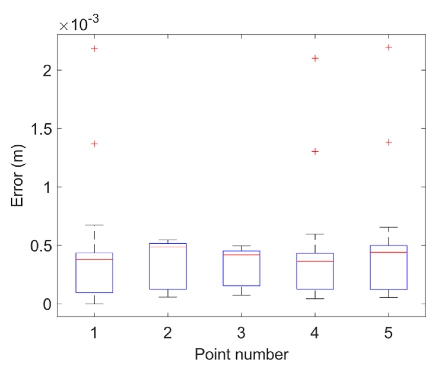
4.3. ISO 9283 Standard

ISO 9283 provides standards for testing an industrial robot for pose repeatability. To have a repeatable test and comparison between the industrial robots, this ISO standard specifies robot mounting conditions, operating and environmental conditions, and instrumentations for the measurements. Test velocities, number of cycles, and test procedures are well defined in this environment. Robotic characteristics that are tested in this environment include pose accuracy and repeatability, transient response of the industrial robot such as positional stabilization time, the amount of overshoot, path following characteristics, and corner round off characteristics. Figure 12 illustrates an ISO 9283 trajectory within a 5 cm cubic workspace. ISO 9283 trajectory is recommended by the standard to be designed within the inner 90% of the overall workspace volume.

Test number 4 is designed as the positioning for five different points selected from an ISO 9283 trajectory. To perform this test, the center of the shape is selected as point number five, and the four other points are numbered from one to four (see Figure 12). The positioning accuracies for the selected points are tested for both open-loop and closed-loop tests. Points number 1–5 as indicated in Figure 12 are generated using Robodk software package using its standard menu and then are used within the Python code to control the industrial robot. Tests are repeated 30 times, and numerical values in terms of the mean values and standard deviations are presented in

Table 3. Positioning error values for test number 4.

	Closed Loop		Open Loop
	Avg. (µm)	Std. (µm)	Avg. (µm)	Std. (µm)
Point 1	45.6	18.2	366.0	439.2
Point 2	48.4	29.9	330.3	204.2
Point 3	54.2	25.1	307.1	159.6
Point 4	45.3	15.9	367.3	411.9
Point 5	45.0	25.8	415.9	433.9

. The numerical values given in Table 3 demonstrate that in using the proposed approach, the positional error is reduced by at least 82% for following the selected points from the ISO 9283 standard. The box-and-whisker plot of the positioning error values for open loop and closed loop are given in Figure 13 and Figure 14, respectively. The red crosses in these images refer to the outliers detected during the statistical analysis. As can be seen from these figures, not only is the mean value of position error reduced for the proposed approach considerably, but also there exists a considerable standard deviation reduction for the position error using the proposed approach. Moreover, the number of outliers observed in the case of closed-loop approach is less compared to the open-loop approach. Therefore, the results of using the proposed approach are more consistent. The movements performed by the linear stage to compensate for the positional error are given in Figure 15, which shows that a few micrometer movements in the linear stage are required to improve the positional accuracy of the overall system. Such very small movements would not be possible without having a precision linear stage in the overall robotic structure. Therefore, results illustrate the effectiveness of the proposed modification made to the robotic structure and the proposed control approach.

5. Conclusions

This paper presents a modification of a six-degrees of freedom (DoF) industrial robot by incorporating a prismatic joint at its end effector, resulting in a 6RP industrial robot, characterized by the integration of six revolute joints and a prismatic joint. The inclusion of this mechanical adaptation enables robot movements with smaller step sizes, as the prismatic joint exhibits a higher resolution of motion. This added feature significantly enhances the overall robot movement resolution. The positioning of the 6RP industrial robot is managed through position feedback facilitated by a laser tracker. The FK of the overall system is identified using an MLPNN, which is subsequently employed to calculate the necessary adjustments in the joint angle values and the displacement of the prismatic joint to enhance positional accuracies of the industrial robot. The position accuracy of the resulting control system is compared against the original industrial robot controller in four different cases. In the first three cases, three different trajectories are defined, and they are used for test purposes. In the last case, five different points chosen from an ISO 9283 trajectory are selected and the position accuracy of the 6RP industrial robot is tested. It is observed that in using the proposed mechanical modification and the proposed positioning algorithm, it is possible to obtain considerable positioning accuracy improvement for the industrial robot. Specifically, for the points extracted from an ISO 9283 trajectory, the proposed method demonstrates an improvement of more than 82% in the positioning accuracy of the 6RP industrial robot when compared to the original industrial robot controller.

As a future work, the proposed approach will be further improved to deal with dynamic trajectory tracking cases. Furthermore, to extend the generality of the proposed approach to a larger area, the stitching approach is chosen. Using a stitching approach, the application of the industrial robot position control, which is valid for a small area, will be extended to a larger area. The performance of the future approach against the ISO 9283 standard will also be investigated.

References

1. Thomas, S.; Rajakumari, R.; George, A.; Kalarikkal, N. Innovative Food Science and Emerging Technologies; CRC Press: Boca Raton, FL, USA, 2018. [Google Scholar]
2. Ansari, R.J.; Karayiannidis, Y. Task-based role adaptation for human-robot cooperative object handling. IEEE Robot. Autom. Lett. 2021, 6, 3592–3598. [Google Scholar]
3. Xu, P.; Cheung, C.F.; Wang, C.; Zhao, C. Novel hybrid robot and its processes for precision polishing of freeform surfaces. Precis. Eng. 2020, 64, 53–62. [Google Scholar]
4. Yin, Y.; Zheng, P.; Li, C.; Wan, K. Enhancing human-guided robotic assembly: AR-assisted DT for skill-based and low-code programming. J. Manuf. Syst. 2024, 74, 676–689. [Google Scholar]
5. Zhang, T.; Peng, F.; Tang, X.; Yan, R.; Deng, R.; Zhao, S. A sparse knowledge embedded configuration optimization method for robotic machining system toward improving machining quality. Robot. Comput. Integr. Manuf. 2024, 90, 102818. [Google Scholar]
6. Wahidi, S.I.; Oterkus, S.; Oterkus, E. Robotic welding techniques in marine structures and production processes: A systematic literature review. Mar. Struct. 2024, 95, 103608. [Google Scholar]
7. Xu, F.; Zi, B.; Yu, Z.; Zhao, J.; Ding, H. Design and implementation of a 7-DOF cable-driven serial spray-painting robot with motion-decoupling mechanisms. Mech. Mach. Theory 2023, 192, 105549. [Google Scholar]
8. Munaro, M.; Antonello, M.; Antonello, M.; Menegatti, E. Continuous mapping of large surfaces with a quality inspection robot. Robot. Auton. Syst. 2022, 156, 104195. [Google Scholar] [CrossRef]
9. PChua, Y.; Ilschner, T.; Caldwell, D.G. Robotic manipulation of food products–a review. Ind. Robot. Int. J. 2003, 30, 345–354. [Google Scholar]
10. Woo, H.M.; Keasling, J. Measuring the economic efficiency of laboratory automation in biotechnology. Trends Biotechnol. 2024, 42, 1076–1080. [Google Scholar]
11. Attanasio, A.; Scaglioni, B.; De Momi, E.; Fiorini, P.; Valdastri, P. Autonomy in surgical robotics. Annu. Rev. Control. Robot. Auton. Syst. 2021, 4, 651–679. [Google Scholar]
12. Du, H.; Wang, G.; Wang, L.; Hao, S.; Fang, Z.; Zhou, H. A closed-loop calibration method for serial robots based on position constraints and local area measurement. Precis. Eng. 2024, 89, 121–134. [Google Scholar]
13. Khanesar, M.A.; Yan, M.; Isa, M.; Piano, S.; Branson, D.T. Precision Denavit–Hartenberg Parameter Calibration for Industrial Robots Using a Laser Tracker System and Intelligent Optimization Approaches. Sensors 2023, 23, 5368. [Google Scholar] [CrossRef] [PubMed]
14. Kluz, R.; Kubit, A.; Trzepiecinski, T. Investigations of temperature-induced errors in positioning of an industrial robot arm. J. Mech. Sci. Technol. 2018, 32, 5421–5432. [Google Scholar]
15. Sigron, P.; Aschwanden, I.; Bambach, M. Compensation of Geometric, Backlash, and Thermal Drift Errors Using a Universal Industrial Robot Model. IEEE Trans. Autom. Sci. Eng. 2023, 21, 6615–6627. [Google Scholar]
16. Ma, S.; Deng, K.; Lu, Y.; Xu, X. Error compensation method of industrial robots considering non-kinematic and weak rigid base errors. Precis. Eng. 2023, 82, 304–315. [Google Scholar]
17. Ueno, Y.; Tachiya, H. Suppressing residual vibration caused in objects carried by robots using a heuristic algorithm. Precis. Eng. 2022, 80, 1–9. [Google Scholar]
18. Aoyagi, S.; Kohama, A.; Nakata, Y.; Hayano, Y.; Suzuki, M. Improvement of robot accuracy by calibrating kinematic model using a laser tracking system-compensation of non-geometric errors using neural networks and selection of optimal measuring points using genetic algorithm. In Proceedings of the 2010 IEEE/RSJ International conference on intelligent robots and systems, Taipei, Taiwan, 30 October–5 November 2010; pp. 5660–5665. [Google Scholar]
19. Bai, M.; Zhang, M.; Zhang, H.; Li, M.; Zhao, J.; Chen, Z. Calibration method based on models and least-squares support vector regression enhancing robot position accuracy. IEEE 2021, 9, 136060–136070. [Google Scholar]
20. Duong, Q.K.; Trang, T.T.; Pham, T.L. Robot Control Using Alternative Trajectories Based on Inverse Errors in the Workspace. J. Robot. 2021, 2021, 1–8. [Google Scholar]
21. Nguyen, H.-N.; Zhou, J.; Kang, H.-J. A calibration method for enhancing robot accuracy through integration of an extended Kalman filter algorithm and an artificial neural network. Neurocomputing 2015, 151, 996–1005. [Google Scholar] [CrossRef]
22. Cao, S.; Cheng, Q.; Guo, Y.; Zhu, W.; Wang, H.; Ke, Y. Pose error compensation based on joint space division for 6-DOF robot manipulators. Precis. Eng. 2022, 74, 195–204. [Google Scholar]
23. Yin, Y.; Gao, D.; Deng, K.; Lu, Y. Vision-based autonomous robots calibration for large-size workspace using ArUco map and single camera systems. Precis. Eng. 2024, 90, 191–204. [Google Scholar]
24. Nguyen, H.-N.; Le, P.-N.; Kang, H.-J. A new calibration method for enhancing robot position accuracy by combining a robot model–based identification approach and an artificial neural network–based error compensation technique. Adv. Mech. Eng. 2019, 11, 1687814018822935. [Google Scholar]
25. Tao, Y.; Liu, H.; Chen, S.; Lan, J.; Qi, Q.; Xiao, W. An Off-Line Error Compensation Method for Absolute Positioning Accuracy of Industrial Robots Based on Differential Evolution and Deep Belief Networks. Electronics 2023, 12, 3718. [Google Scholar] [CrossRef]
26. ISO 9283-1998; Manipulating Industrial Robots Performance Criteria and Related Test Methods. ISO: Geneva, Switzerland, 1998.
27. Robodk. 5 March 2025. Available online: https://robodk.com/doc/en/Robot-Validation-ISO9283.html (accessed on 22 March 2025).
28. ISO 10218-1:2011; Robot for Industrial Environments—Safety Requirements—Part 1: Robot. Technical Report; International Organization for Standardization: Geneva, Switzerland, 2006.
29. ISO 10218-2:2011; Robots and Robotic Devices—Safety Requirements for Industrial Robots—Part 2: Robot Systems and Integration. International Organization for Standardization: Geneva, Switzerland, 2011.
30. Kufieta, K. Force Estimation in Robotic Manipulators: Modeling, Simulation and Experiments; Department of Engineering Cybernetics NTNU Norwegian University of Science and Technology: Trondheim, Norway, 2014. [Google Scholar]
31. Sun, J.-D.; Cao, G.-Z.; Li, W.-B.; Liang, Y.-X.; Huang, S.-D. Analytical inverse kinematic solution using the DH method for a 6-DOF robot. In Proceedings of the 2017 14th international conference on ubiquitous robots and ambient intelligence (URAI), Jeju, Republic of Korea, 28 June–1 July 2017; pp. 714–716. [Google Scholar]
32. Chen, T.; Lin, J.; Wu, D.; Wu, H. Research of calibration method for industrial robot based on error model of position. Appl. Sci. 2021, 11, 1287. [Google Scholar] [CrossRef]
33. Pollák, M.; Kočiško, M.; Paulišin, D.; Baron, P. Measurement of unidirectional pose accuracy and repeatability of the collaborative robot UR5. Adv. Mech. Eng. 2020, 12, 1687814020972893. [Google Scholar] [CrossRef]
34. Wu, X. Analysis of robot joint rotation error for manufacturing and mechatronics integration. Int. J. Interact. Des. Manuf. IJIDeM 2024, 18, 2503–2516. [Google Scholar]
35. Khanesar, M.A.; Piano, S.; Branson, D. Uncertainty analysis of an augmented industrial robot. In Proceedings of the Joint Special Interest Group Meeting between Euspen and ASPE Advancing Precision in Additive Manufacturing, Leuven, Belgium, 19–21 September 2023. [Google Scholar]
36. Dusek, J.E.; Triantafyllou, M.S.; Lang, J.H. Piezoresistive foam sensor arrays for marine applications. Sens. Actuators A Phys. 2016, 248, 173–183. [Google Scholar] [CrossRef]
37. Castellanos-Ramos, J.; Navas-González, R.; Fernández, I.; Vidal-Verdú, F. Insights into the mechanical behaviour of a layered flexible tactile sensor. Sensors 2015, 15, 25433–25462. [Google Scholar] [CrossRef]
38. Arrington, C.B.; Rau, D.A.; Williams, C.B.; Long, T.E. UV-assisted direct ink write printing of fully aromatic Poly (amide imide) s: Elucidating the influence of an acrylic scaffold. Polymer 2021, 212, 123306. [Google Scholar]
Figure 1. MLPNN structure.
Robotics 14 00042 g001
Figure 2. The flowchart of the proposed precision positioning of the robot.
Robotics 14 00042 g002
Figure 3. Overall experimental setup.
Robotics 14 00042 g003
Figure 4. Connectivity diagram for the experimental setup.
Robotics 14 00042 g004
Figure 5. The convergence graph for the MLPNN using Levenberg−Marquardt training algorithm.
Robotics 14 00042 g005
Figure 6. The R2 regression analysis for the MLPNN using Levenberg–Marquardt training algorithm.
Robotics 14 00042 g006
Figure 7. (a) MLPNN output versus target position values in x-axis; (b) MLPNN output versus target position values in y-axis; and (c) MLPNN output versus target position values in z-axis.
Robotics 14 00042 g007
Figure 8. (a) Trajectory following experiment 1. (b) Trajectory following experiment 2. (c) Trajectory following experiment 3.
Robotics 14 00042 g008
Figure 9. (a) Error values for open–loop case of experiment 1. (b) Error values for closed–loop case of experiment 1.
Robotics 14 00042 g009
Figure 10. (a) Error values for open–loop case of experiment 2. (b) Error values for closed–loop case of experiment 2.
Robotics 14 00042 g010
Figure 11. (a) Error values for open–loop case of experiment 3. (b) Error values for closed–loop case of experiment 3.
Robotics 14 00042 g011
Figure 12. ISO 9283 trajectory (in yellow) for UR5 within the investigated workspace.
Robotics 14 00042 g012
Figure 13. Open–loop errors for test number 4.
Robotics 14 00042 g013
Figure 14. Closed–loop errors for test number 4.
Robotics 14 00042 g014
Figure 15. Move stage movements for test number 4.
Robotics 14 00042 g015