Real Time MEMS-Based Joint Friction Identification for Enhanced Dynamic Performance in Robotic Applications

Abstract

The mechatronic design approach to robotics deploys, inter alia, widely available mechanical design engineering tools that, together with standard production techniques, allow the accurate quantification of the system’s mass properties. While this enables the synthesis of model-based centralized controllers, friction still limits the achievable dynamic performances, as its prediction at the design stage is hampered by complex dependencies on loads, temperature, wear, and lubrication. Further uncertainties affecting mechatronic devices stem from the actuation systems, whose parameters are specified by the manufacturer with relatively loose accuracy. These challenges are addressed here through a method based on MEMS IMUs for the real-time estimation of both friction effects and uncertain actuator parameters. The resulting model, inclusive of the frictionless dynamics, is applied in a closed loop to improve the control performance. An experimental comparison with decentralized and non-adaptive regulators highlights severalfold reductions in tracking errors; the ability to track temperature-dependent friction variations is also shown. From this work, it may be concluded that the use of MEMS sensors, together with identification and adaptive control algorithms, sensibly increases the dynamic performance of robotic systems. The real-time properties of the method also enable future investigations into topics such as MEMS-based diagnostics and predictive maintenance.

1. Introduction

Robotic devices are multi-domain systems with a tight integration of mechanical, actuation, measurement, control, and algorithmic components. Being mechatronic systems, their development process follows the mechatronic approach, which presents significant opportunities for design streamlining and performance maximization due to its interdisciplinary nature. The method uses, among others, widely available mechanical design engineering tools that, combined with standard production techniques, allow, in particular, a high-confidence estimation of the mechanical elements’ moving masses; this knowledge, together with the simulation of the actual tasks to be performed by the machine, enables, in turn, the proper selection of transmission and actuation systems [1], the estimation of the achievable productivity profile [2], and the implementation of more effective centralized control systems [3,4]. Given an accurate model of the robot, centralized controllers are indeed able to compensate for both gravitational and inertial loads, whose relative relevance depends on the nature of the robot and the application. Another important source of mechanical loads is, however, constituted by friction, whose accurate modelling still remains challenging due to complex dependencies on temperature [5], lubrication conditions [6], wear [7,8,9], preloads [10], and applied forces. All these factors complicate the selection of the form and parameters of the friction model, and in fact, despite considerable research efforts in different applications (e.g., multibody system simulation [11] or advanced control algorithms), none has gained universal acceptance. Considering two nominally identical robots, in [12], it is shown experimentally that the actual frictional behaviour in each individual joint is unique, thus highlighting the limitations of non-data-driven friction modelling. Despite these difficulties, friction and its compensation are particularly relevant for high-performance devices, which typically use preloaded mechanical joints that ensure stiffness and null backlash, but also induce significant frictional actions.

Accordingly, the experimental estimation of unknown inertial and friction parameters that characterize mechanical systems has been long recognized as a relevant research topic. Two basic approaches are possible: either identification or adaptive control. The main difference between the two lies in the fact that, in adaptive control, the model estimation and deployment times coincide, whereas they remain separate under identification-based methods. As a result, the latter may exploit offline signal processing techniques such as non-causal filters, whereas the former may rely on more constrained online data processing; on the other hand, the adaptive mechanism allows us to track slow changes in the system’s parameters during its normal operation. In robotic applications, both methods classically exploit the linearity of the dynamics equations with respect to the inertial parameters of the system, which if unknown, can then be estimated using well-established numerical methods.

Friction models may also be characterized by linearity with respect to their parameters, while still accounting for the marked non-linearity of the friction phenomena using appropriate shape functions; as such, they are able to capture most of the features associated with friction such as stiction, the Stribeck effect, and a high-order dependency on velocity, all the while remaining simple and computationally efficient. This latter property is especially desirable for methods that are executed in real time, in parallel to the utilization of the robot for the execution of its intended tasks.

More complex modelling approaches are characterized by non-linearity; due to the fact that their parametric form involves algebraic functions only, they still belong to the class of static models. Recent examples of their use for friction identification on serial robot arms are found in [13,14]. Non-linear, static friction models for adaptive compensation have also been built using artificial neural networks in works such as [15,16], which demonstrate, in simulated settings and for a single servo-actuated link, techniques that guarantee convergence during the network training; in these works, transmission elasticities are also considered.

Finally, the most sophisticated friction models, beyond memoryless non-linearities, also introduce state variables and corresponding observers to account for friction phenomena such as pre-sliding, stick–slip, and hysteresis. In this class, pioneering work has led to the development of the LuGre model [17], which has since been widely applied. Extensions of this model allow its use for online friction estimation and compensation and also in the case of friction variations induced by applied loads and temperature changes, as demonstrated experimentally on a single DOF DC motor servomechanism in [18]. A dynamic friction model with temperature dependency is also used for adaptive control in simulated settings in [19].

Two other dynamic friction models, one historically preceding and the other following the LuGre formulation, are the well-known Dahl [20] and Leuven [21,22] models. Given this variety of friction models, a choice among them should be made considering factors such as straightforwardness, robustness, accuracy, and appropriateness for the intended application. Linear, static models are undoubtedly the simplest; moreover, due to their mathematical structure, the estimation of their parameters is also straightforward. Concerning accuracy, several contributions are available in the literature: Focusing on micro stick–slip motion systems, ref. [23] proposes an interesting experimental comparison between five different static and dynamic friction models, leading to the conclusion that, for the considered application, the LuGre model performs best. On the other hand, the experimental analysis performed in [24] suggests that for the specific case study, which focuses on low-velocity tracking, both the Dahl and the Leuven models outperform the LuGre model. Finally, in [25], another comparative and experimental study, the LuGre model is found, in general, to be the best performing; however, the proposed comparison takes into account different application requirements, leading to the conclusion that, for the analysis of gross motions, where velocity-dependent terms dominate, both the LuGre and considered static models are appropriate.

Historically, difficulties in obtaining direct acceleration measurements have led to the development of accelerometer-free adaptive control methods (e.g., see [26,27]), which place more emphasis on the direct minimization of tracking errors and which have received more attention than coeval acceleration-based schemes [28]. In the ensuing decades, however, due to traction from the consumer electronics sector, MEMS Inertial Measurement Units (IMUs) were developed into accessible and increasingly sophisticated sensors that also found widespread applications in robotics to complement the always-available position transducers such as rotary encoders or resolvers. MEMS accelerometers have indeed been used in mobile robots to aid the solution of problems such as attitude estimation [29,30], terrain classification [31], and odometry [32,33]. Attitude estimation solved with MEMS accelerometers is also widespread in UAV applications [34,35]. In fixed robotics, MEMS accelerometers have been used for collision detection, e.g., in [36,37], and for link velocity and acceleration estimation [38]. Despite these developments, until now, sensorless friction identification methods have been often preferred. In [39], an observer-based virtual sensor for joint friction identification is developed to avoid torque and acceleration measurements; the resulting technique is applied to a simple 1-DOF experimental setup. Somewhat similarly, ref. [40] uses Time-Delay Estimation to compensate for friction and contact forces on a 2-DOF SCARA; an interesting experimental validation that included contact forces and robot–robot cooperation is presented. In [41], a new algorithm for friction identification is developed and applied to a single joint of a serial manipulator; the identification was performed offline, and the friction model was not ultimately used in a control loop for friction compensation. Another sensorless method, based on extended Kalman filtering and Bayesian optimization, is presented in [42] and applied to a 6-DOF serial manipulator operating under Cartesian impedance control. In [43], the influence of temperature and external loads on friction is experimentally investigated on a 6-DOF robot arm. The friction estimation is carried out under controlled settings, taking care to move in isolation and at constant speed for each joint, while also configuring the others in such a way as to exclude gravitational actions on the studied joint. The resulting friction model is then introduced in the control system, highlighting its benefits in terms of achieved tracking accuracy. A similar work is presented in [44], where temperature effects were also considered. The work discussed in [45] describes the offline identification of the friction parameters of a 3-DOF planar SCARA-like robot using a linear least square method based on a polynomial friction model; while the experimental results are described, no mention is made on the method used for acceleration estimation.

From the analysis of these papers, it emerges that whenever an offline identification approach is chosen, special care is used in the selection of the motions to be performed by the robotic device; at the same time, the problem of acceleration measurement is not keenly felt due to the availability of offline data processing options. Recently proposed online methods [46,47] also put more emphasis on the avoidance of additional sensors, due to the fact that these are rarely provided as a standard option by manufacturers of industrial robots.

Despite this tendency, the several applications of MEMS accelerometers, especially in mobile robotics, attest to the fact that the use of these sensors can lead to significant benefits at a negligible cost. In particular, a promising application of direct acceleration measurement in industrial robotics is the real-time identification of friction for motion control performance improvement. When a current or torque mode controller is available, both the torque inputs and the acceleration response may be directly used to infer the parameters of a suitable friction model, which, in turn, can be included in a control scheme, e.g., in the form of a torque feedforward or of a feedback linearization term, to enhance the performance of the manipulator. An example of this concept can be found in the recent work of [48], in which both offline and online identification methods based on IMUs are considered.

This paper presents a general method based on MEMS accelerometers and gyroscopes for the real-time, closed-loop estimation of both friction effects and uncertain driver and actuator parameters. The method allows the estimation of the joints’ friction for both serial and parallel kinematic robot configurations. The paper also presents the experimental validation of the proposed procedure using a 5R parallel kinematic manipulator. One of the objectives is the estimation of the uncertain friction parameters during the normal functioning of the device, that is, without introducing special trajectories optimized for identification but unrelated to the robot’s actual task. An equally important goal is the use of the estimated friction model to improve the dynamic performance of the system in terms of tracking errors. A key tool is the exploitation of direct acceleration measures to precisely identify sliding and stiction conditions; in the former, frictional actions can be assumed to be mainly velocity-dependent, whereas in the latter, friction generates constraint reactions that balance the applied torques in a statically undetermined way in the case of mechanisms displaying closed kinematic chains.

Given this distinction, during sliding conditions, the measurement of position, velocity, acceleration, and applied torque can, in principle, be used to single out the friction actions arising from the relative motion of mechanical elements. Caution should, however, be exercised, inasmuch as the torque measurements performed by motor drivers are not direct ones [49], and are, in particular, affected by tolerances and deviations both of the driver’s sensing components and of the motor windings. The uncertainties associated with each power drive system (PDS), i.e., the driver–actuator pair, result, in particular, in a non-unitary static gain from the desired to the actual torque; this torque conversion gain, whose presence is undetectable considering only the measure provided by the driver, is explicitly considered in the proposed dynamic model of the manipulator and included among the to-be-identified parameters. On the other hand, the masses and inertias will be considered as known quantities to be used as the ground truth for the subsequent estimation of the unknown terms. These unusual assumptions are motivated by the point of view adopted for this work, which is that of the designer of the robot and not that of the final user.

Therefore, compared to related works that focus on offline friction identification or online adaptive control, the main distinctive elements of the present paper are as follows:

• The proposed method does not rely on the sequential, joint-by-joint friction analysis often performed on serial robots; therefore, it is applicable not only to serial kinematic chains but also to parallel chains.
• The identification process is carried out in real time on multi-axis systems during normal motion tasks and without using specially designed trajectories.
• Focus is placed on the uncertain friction and PDS parameters, as the masses are already known.
• In particular, a rarely considered source of uncertainty, namely, the actual value of each PDS torque conversion gain, is explicitly considered in the proposed formulation.
• Finally, the stiction regime is detected using accelerometric and gyroscopic measures and excluded from the identification process, as the velocity-based friction model is not applicable in those conditions.

Accordingly, the main contributions are as follows:

• The development of a low-cost solution for a real-time friction identification architecture, based on MEMS IMUs applicable to multi-DOF serial and parallel mechanisms alike;
• The theoretical analysis and subsequent compensation of the effects of uncertain PDS parameters;
• An empirical and comparative demonstration of the benefits achievable with the proposed measurement, identification, and control architecture in realistic, high-speed pick-and-place motion cycles.
• An experimental characterization of the frictional phenomena on a high stiffness 5R parallel kinematic robot that also includes an analysis of the effects of temperature both on friction and on its identification.

Concerning pioneering papers such as [18], the novelty of this paper is the real-time multi-joint friction identification of multi-axis systems using a non-linear centralized control algorithm to enhance the system’s overall dynamic performances. Moreover, the proposed approach considers the uncertainties introduced by the electric actuators and uses MEMS sensors for the friction identification process, bypassing the need for observers and leading to fast convergence. Given the analysis described in [25], a static, velocity-based friction model is adopted due to the fact that the present work is focused on highly dynamic applications characterized by large displacements in which high accelerations and speeds are prevalent. The paper is structured as follows: Section 2 describes, in general terms, the proposed identification and control architecture, considering both software and hardware requirements; the selected case study for the first application of the method is subsequently presented in detail in Section 3, both in terms of mathematical modelling and experimental setup; and the main experimental findings are then illustrated and discussed. Finally, in Section 4, the conclusions of this work are stated; further lines of inquiry naturally following the present investigation are eventually suggested.

2. Methods

Typical methods used to model the mechanical dynamics of multi-DOF rigid-body systems result in equations of motion of the following form:

$$\begin{array}{c}\hfill \mathit{M}\left(\mathit{q}\right)\ddot{\mathit{q}}+\mathit{C}\left(\mathit{q},\dot{\mathit{q}}\right)\dot{\mathit{q}}+\nabla U\left(\mathit{q}\right)={\mathit{Q}}_{\mathit{m}}(\mathit{q},{\mathit{\tau }}_{\mathit{m}})+{\mathit{Q}}_{\mathit{F}}(\mathit{q},\dot{\mathit{q}}).\end{array}$$

(1)

On the left-hand side of Equation (1), $\mathit{q}$ is the vector containing the $n_{dof}$ generalized coordinates chosen to describe the system, while $\dot{\mathit{q}}$ and $\ddot{\mathit{q}}$ are its first and second time derivatives; $\mathit{M}\left(\mathit{q}\right)$, $\mathit{C}\left(\mathit{q},\dot{\mathit{q}}\right)$ and $\nabla U\left(\mathit{q}\right)$ are, respectively, the mass matrix, the matrix associated with centrifugal and Coriolis actions, and the gradient of the potential energy with respect to $\mathit{q}$. On the right-hand side, ${\mathit{Q}}_{\mathit{m}}$ and ${\mathit{Q}}_{\mathit{F}}$ denote the Lagrangian components associated, respectively, to the motor torques ${\mathit{\tau }}_{\mathit{m}}$ and to the frictional actions arising as a result of relative motions within the mechanism’s $n_j$ joints. Of note is the dependency of ${\mathit{Q}}_{\mathit{m}}$ on $\mathit{q}$, which is due to the transmission system interposed between the motors and the generalized coordinates. Denoting then the rotations of the motor shafts with ${\mathit{q}}_m$ and the Jacobian matrix with ${\mathit{D}}_{\mathit{m}}\left(\mathit{q}\right)$ such that ${\dot{\mathit{q}}}_{\mathit{m}}={\mathit{D}}_{\mathit{m}}\left(\mathit{q}\right)\dot{\mathit{q}}$, the following may be written:

$$\begin{array}{c}\hfill {\mathit{Q}}_{\mathit{m}}(\mathit{q},{\mathit{\tau }}_{\mathit{m}})={\mathit{D}}_{\mathit{m}}{\left(\mathit{q}\right)}^{\top }{\mathit{\tau }}_{\mathit{m}},\end{array}$$

(2)

which highlights the linearity of ${\mathit{Q}}_{\mathit{m}}$ with respect to ${\mathit{\tau }}_{\mathit{m}}$. As the Lagrangian components of the inertial and of the gravitational actions are, respectively,

$$\begin{array}{cc}\hfill {\mathit{Q}}_{\mathit{I}}(\mathit{q},\dot{\mathit{q}},\ddot{\mathit{q}})& =-\left(\mathit{M}\left(\mathit{q}\right)\ddot{\mathit{q}}+\mathit{C}(\mathit{q},\dot{\mathit{q}})\dot{\mathit{q}}\right)\hfill \end{array}$$

(3)

$$\begin{array}{cc}\hfill {\mathit{Q}}_{\mathit{G}}\left(\mathit{q}\right)& =-\nabla U\left(\mathit{q}\right),\hfill \end{array}$$

(4)

Equation (1) may then be rewritten as follows:

$$\begin{array}{c}\hfill {\mathit{Q}}_{\mathit{m}}(\mathit{q},{\mathit{\tau }}_{\mathit{m}})+{\mathit{Q}}_{\mathit{F}}(\mathit{q},\dot{\mathit{q}})+{\mathit{Q}}_{\mathit{I}}(\mathit{q},\dot{\mathit{q}},\ddot{\mathit{q}})+{\mathit{Q}}_{\mathit{G}}\left(\mathit{q}\right)=\mathbf{0}.\end{array}$$

(5)

For identification and adaptive control purposes, ${\mathit{Q}}_{\mathit{I}}$ and ${\mathit{Q}}_{\mathit{G}}$ are typically expressed in regression form, i.e., in a way that highlights their linearity with respect to the mass (or inertial) parameters of the mechanical system. Within the scope of this paper, there is, however, no need to estimate these quantities, since their accurate quantification is assumed to be already available as a by-product of the mechanical design process of the mechanism. An exception can, in principle, be made for the robot’s payload, which is seldom known in advance and possibly not constant due to the wide array of possible employment methods of the device. Depending on the type of robot, however, the payload mass can be expected to remain negligible compared to that of the manipulator itself; this is the case for the example of highly dynamic applications. In other situations, where the payload is a significant fraction of the total mass, slower movements are to be anticipated, together with motion cycles long enough to allow the online estimate of the additional masses, as carried out, for example, in [50]. This problem will not be explicitly treated in this work, even though its solution could be integrated into the proposed methods by splitting the known and constant inertial and mass parameters from those related to the unknown and time-varying payload. For the sake of compactness, in the following discussion, a negligible or known payload mass will be assumed; any form that allows the evaluation of ${\mathit{Q}}_{\mathit{G}}$ and ${\mathit{Q}}_{\mathit{I}}$ is then acceptable. On the other hand, greater scrutiny than typically reserved to ${\mathit{Q}}_{\mathit{m}}$ is warranted. In fact, for electrically actuated manipulators, the measurement of the motor torque ${\mathit{\tau }}_{\mathit{m}}$ is indirectly obtained from the electrical quantities observed by the drivers, and furthermore, it requires an estimate of each motor’s torque constant. The manufacturing tolerances of each driver’s sensing components and each motor winding are therefore explicitly considered in the following discussion as multiplicative uncertainties induced by each PDS (i.e., the driver–motor unit) of the following type:

$$\begin{array}{c}\hfill {\mathit{\tau }}_{\mathit{m}}=\mathrm{diag}\left({\check{\mathit{\tau }}}_{\mathit{m}}\right){\mathit{\pi }}_{\mathit{pds}},\end{array}$$

(6)

with ${\check{\mathit{\tau }}}_{\mathit{m}}$ being the driver-provided measure of the motor torques and ${\mathit{\pi }}_{\mathit{pds}}$ being a vector of unknown scale parameters. Defining then ${\mathit{Y}}_{\mathit{pds}}(\mathit{q},{\check{\mathit{\tau }}}_{\mathit{m}})=-{\mathit{D}}_{\mathit{m}}{\left(\mathit{q}\right)}^{\top }\mathrm{diag}\left({\check{\mathit{\tau }}}_{\mathit{m}}\right)$, Equation (2) may be rewritten as follows:

$$\begin{array}{c}\hfill {\mathit{Q}}_{\mathit{m}}=-{\mathit{Y}}_{\mathit{pds}}(\mathit{q},{\check{\mathit{\tau }}}_{\mathit{m}}){\mathit{\pi }}_{\mathit{pds}}.\end{array}$$

(7)

Concerning, on the other hand, the problem of friction identification, it is first of all necessary to derive the Lagrangian components ${\mathit{Q}}_{\mathit{F}}$ of the friction torques (or forces) ${\tau }_{F,j}$ that arise in the mechanism’s joints as a result of the $n_{\upsilon }$ relative velocities ${\dot{\upsilon }}_j$ between connected links. It may be noted that, in serial kinematic chains, $n_{\upsilon }$ coincides with the number $n_j$ of joints, all of which are actuated; on the other hand, for parallel kinematic robots (PKRs), each joint (e.g., a revolute, spherical, or universal one) may be active or passive and may allow a plurality of relative motions, resulting in a number $n_{\upsilon }$ usually greater than $n_j$. Typically, actuated joints display greater friction due to the presence of gearboxes; passive joints are often less critical, but in specific applications, they may also induce significant dissipations either because of high preloads or due to the presence of gaskets and seals.

Irrespective of these distinctions, the friction torques or forces are purely dissipative, and their work may be computed considering the relative displacements ${\upsilon }_j$. Their overall virtual work can therefore be written as follows:

$$\begin{array}{c}\hfill \delta L_F=\delta {\mathit{q}}^{\top }{\displaystyle \sum _{j=1}^{n_{\upsilon }}}{\mathit{D}}_{{\upsilon }_j}^{\top }\left(\mathit{q}\right){\mathit{\tau }}_{F,j},\end{array}$$

(8)

in which ${\mathit{D}}_{{\upsilon }_j}$ is the Jacobian associated with ${\upsilon }_j\left(\mathit{q}\right)$ such that ${\dot{\upsilon }}_j={\mathit{D}}_{{\upsilon }_j}\left(\mathit{q}\right)\dot{\mathit{q}}$. As a result, the frictional Lagrangian components are as follows:

$$\begin{array}{c}\hfill {\mathit{Q}}_{\mathit{F}}={\displaystyle \sum _{j=1}^{n_{\upsilon }}}{\mathit{D}}_{{\upsilon }_j}^{\top }\left(\mathit{q}\right){\mathit{\tau }}_{F,j}.\end{array}$$

(9)

Within this work, each friction torque or force is assumed to depend linearly on a set of unknown parameters; without loss of generality, a symmetric polynomial friction model of order w has, in particular, been adopted:

$$\begin{array}{c}\hfill {\tau }_{F,j}=\mathrm{sign}\left({\dot{\upsilon }}_j\right)\left[\begin{array}{ccccc}1& \left|{\dot{\upsilon }}_j\right|& {\left|{\dot{\upsilon }}_j\right|}^2& \dots & {\left|{\dot{\upsilon }}_j\right|}^w\end{array}\right]{\mathit{\pi }}_{\mathit{F},j}.\end{array}$$

(10)

Such a model can describe the friction profiles most commonly occurring in high-performance mechanical components suitable for robotic applications, which typically display symmetric frictional behaviour. Indeed, as the selected shape functions are all odd, the friction model will be characterized by the same property. If required by other contexts, an asymmetric friction model of the same order could also, however, be easily derived at the cost of a doubled number of parameters. Regardless of this or other possible variants, the form of the friction regressor ${\mathit{Y}}_{\mathit{F}}(\mathit{q},\dot{\mathit{q}})$ is written such that

$$\begin{array}{c}\hfill {\mathit{Q}}_{\mathit{F}}=-{\mathit{Y}}_{\mathit{F}}(\mathit{q},\dot{\mathit{q}}){\mathit{\pi }}_{\mathit{F}}\end{array}$$

(11)

can be straightforwardly derived, column by column, considering Equations (9) and (10) (or an analogous one) and a vector of unknown friction parameters ${\mathit{\pi }}_{\mathit{F}}$ defined as follows:

$$\begin{array}{c}\hfill {\mathit{\pi }}_{\mathit{F}}={\left[\begin{array}{cccc}{\mathit{\pi }}_{\mathit{F},1}^{\top }& {\mathit{\pi }}_{\mathit{F},2}^{\top }& \dots & {\mathit{\pi }}_{\mathit{F},n_{\upsilon }}^{\top }\end{array}\right]}^{\top }.\end{array}$$

(12)

Given Equations (7) and (11), Equation (5) may then be rewritten and rearranged as follows:

$$\left[\begin{array}{c}{\mathit{Y}}_{\mathit{pds}}(\mathit{q},{\check{\mathit{\tau }}}_{\mathit{m}}),{\mathit{Y}}_{\mathit{F}}(\mathit{q},\dot{\mathit{q}})\end{array}\right]\left[\begin{array}{c}{\mathit{\pi }}_{\mathit{pds}}\\ {\mathit{\pi }}_{\mathit{F}}\end{array}\right]=\mathit{Y}(\mathit{q},\dot{\mathit{q}},{\check{\mathit{\tau }}}_{\mathit{m}})\mathit{\pi }={\mathit{Q}}_{\mathit{I}}(\mathit{q},\dot{\mathit{q}},\ddot{\mathit{q}})+{\mathit{Q}}_{\mathit{G}}\left(\mathit{q}\right).$$

(13)

The right-hand side $\mathit{R}={\mathit{Q}}_{\mathit{I}}+{\mathit{Q}}_{\mathit{G}}$ is a function of the position, velocity, and acceleration conditions, whereas the matrix $\mathit{Y}$ is a function of position $\mathit{q}$, velocity $\dot{\mathit{q}}$, and measured motor torques ${\check{\mathit{\tau }}}_{\mathit{m}}$. It may be remarked here that, in the context of modern electrically actuated industrial robots, both the positions and indirect torque measurements are a strict necessity, even though the manufacturer might not expose them to the final user. Velocities and accelerations are typically not provided, but may be nowadays conveniently obtained from MEMS triaxial gyroscopes and accelerometers integrated into a single IMU and mounted as required on some or all robot links. Due to the structure of Equation (13), given a sequence of $n_s$ sampled data points (with the product $n_s{n}_{dof}$ greater than the dimensionality $n_{\pi }$ of $\mathit{\pi }$), a least square (LS) estimate $\widehat{\mathit{\pi }}$ of the unknown parameters can be obtained.

Within this work, however, instead of using an ordinary offline LS estimation on batch data, an Exponentially Weighted Regularized Recursive LS (EWR–RLS) algorithm was selected to estimate, in real time, the unknown parameters as data are acquired. Moreover, the actually used regressor and right-hand side are ${\mathit{Y}}_{\sum }$ and $R_{\sum }$, each obtained by summing the rows of $\mathit{Y}$ and $\mathit{R}$, respectively. These choices result in several advantages:

• Computational efficiency, as the Woodbury–Sherman–Morrison formula can then be used to avoid matrix inversions altogether;
• Storage efficiency, as new data points are processed at once to yield a running estimate of the unknown parameters and then overwritten;
• Immediate usability of the estimated parameters within the robot’s control system;
• Ability to track slow changes in the parameters (such as those caused, for example, by temperature variations) thanks to the exponentially decaying weighting of the data points;
• Uniqueness of the solution at each iteration.

Concerning the last two points, it may be remarked that, with this algorithm, at time $t_{n_s}$, the estimated parameters correspond to those that minimize the cost function:

$$\begin{array}{c}\hfill J\left(\mathit{\pi }\right)={\displaystyle \frac{1}{2}}\left({\displaystyle \sum _{k=1}^{n_s}}{\beta }^{n_s-k}{\left|\right|({\mathit{Y}}_{\sum }({\mathit{q}}_{\mathit{k}},{\dot{\mathit{q}}}_{\mathit{k}},{\check{\mathit{\tau }}}_{\mathit{m},\mathit{k}})\mathit{\pi }-R_{\sum }({\mathit{q}}_k,{\dot{\mathit{q}}}_k,{\ddot{\mathit{q}}}_k)\left|\right|}^2+{\beta }^{n_s}\lambda {\mathit{\pi }}^{\top }\mathit{\pi }\right),\end{array}$$

(14)

in which $\lambda$ is the regularization parameter and $\beta$ is the forgetting factor. The forgetting factor $\beta \le 1$ introduces an exponential weighting that progressively reduces the influence of older data; given a sample rate $T_s$, its value may be chosen in order to obtain a weighting half-life $T_{HL}$ according to the formula $\beta =1+T_{s}ln\left(0.5\right)/T_{HL}$. In turn, $T_{HL}$ can be selected in relation to the time span in which the data are expected to remain relevant. The selection of $\lambda$ appears to be less critical since, in practice, it is used for the initialization of the EWR-RLS state, but its relevance progressively wanes as more data are acquired due to it being premultiplied by ${\beta }^{n_s}$, which decreases as $n_s$ grows. For the experimental activities described in the following section, the EWR-RLS algorithm is configured specifically with $\lambda =0.001$ and $T_{HL}=600 \mathrm{s}$. Further implementation details may be found, for example, in [51]. As a final note, given the already introduced distinction between the stiction and sliding regime, the data points actually used to update the vector $\widehat{\mathit{\pi }}$ are those for which either the measured accelerations or velocities exceed, in absolute value, a small threshold. This removes any undue influence of data acquired in stiction conditions and ensures that the velocity-based friction model is applied only when actually appropriate.

Figure 1 depicts the overall control architecture developed for this work. The control scheme is of the computed torque kind, in which the inertial and gravitational feedforward contributions ${\mathit{\tau }}_{\mathit{m},{\mathit{I}}_{\mathit{FF}}}$ and ${\mathit{\tau }}_{\mathit{m},{\mathit{G}}_{\mathit{FF}}}$ are determined from the position, velocity, and acceleration setpoints ${\mathit{q}}_{\mathit{sp}}$, ${\dot{\mathit{q}}}_{\mathit{sp}}$, ${\ddot{\mathit{q}}}_{\mathit{sp}}$, given the a priori frictionless dynamic model of the manipulator. The friction feedforward ${\mathit{\tau }}_{\mathit{m},{\mathit{F}}_{\mathit{FF}}}$ is instead dependant not only on ${\mathit{q}}_{\mathit{sp}}$ and ${\dot{\mathit{q}}}_{\mathit{sp}}$, but also on the EWR–RLS estimate ${\widehat{\mathit{\pi }}}_{\mathit{F}}$ of the friction parameters; these may be initialized to a first guess value obtained, for example, from previous runs, or, in the absence of any prior information, to zero. The torque command ${\mathit{\tau }}_{\mathit{m},\mathit{cmd}}$, which features both feedback and feedforward components, is thus defined as follows:

$$\begin{array}{c}\hfill {\mathit{\tau }}_{\mathit{m},\mathit{cmd}}={\mathit{\tau }}_{\mathit{m},{\mathit{G}}_{\mathit{FF}}}+{\mathit{\tau }}_{\mathit{m},{\mathit{I}}_{\mathit{FF}}}+{\mathit{\tau }}_{\mathit{m},{\mathit{F}}_{\mathit{FF}}}+{\mathit{K}}_{\mathit{P}}({\mathit{q}}_{\mathit{sp}}-\mathit{q})+{\mathit{K}}_{\mathit{D}}({\dot{\mathit{q}}}_{\mathit{sp}}-\dot{\mathit{q}}),\end{array}$$

(15)

in which ${\mathit{K}}_{\mathit{P}}$ and ${\mathit{K}}_{\mathit{D}}$ are two diagonal gain matrices. In turn, the feedforward contributions are computed as follows:

$$\begin{array}{cc}\hfill {\mathit{\tau }}_{\mathit{m},{\mathit{G}}_{\mathit{FF}}}& =-{\mathit{D}}_{\mathit{m}}^{-\top }\left({\mathit{q}}_{\mathit{sp}}\right){\mathit{Q}}_{\mathit{G}}\left({\mathit{q}}_{\mathit{sp}}\right)\hfill \end{array}$$

(16)

$$\begin{array}{cc}\hfill {\mathit{\tau }}_{\mathit{m},{\mathit{I}}_{\mathit{FF}}}& =-{\mathit{D}}_{\mathit{m}}^{-\top }\left({\mathit{q}}_{\mathit{sp}}\right){\mathit{Q}}_{\mathit{I}}({\mathit{q}}_{\mathit{sp}},{\dot{\mathit{q}}}_{\mathit{sp}},{\ddot{\mathit{q}}}_{\mathit{sp}})\hfill \end{array}$$

(17)

$$\begin{array}{cc}\hfill {\mathit{\tau }}_{\mathit{m},{\mathit{F}}_{\mathit{FF}}}& ={\mathit{D}}_{\mathit{m}}^{-\top }\left({\mathit{q}}_{\mathit{sp}}\right){\mathit{Y}}_{\mathit{F}}({\mathit{q}}_{\mathit{sp}},{\dot{\mathit{q}}}_{\mathit{sp}}){\widehat{\mathit{\pi }}}_{\mathit{F}}.\hfill \end{array}$$

(18)

The estimated parameters ${\widehat{\mathit{\pi }}}_{\mathit{pds}}$, which, in the absence of any data, could be reasonably initialized to one, are, on the other hand, used as a scale factor to compensate for the torque measurement inaccuracy introduced by the power drive systems due to tolerances on their sensing components and on the nominal values assigned to the motor torque constants. Concerning this point, the grey area in Figure 1 represents an expanded view of a prototypical current loop implemented within the electric driver. In particular, the target torque signal ${\tau }_{m,tgt,j}$ is converted into a current target $i_{tgt,j}$ using a fixed a priori estimate ${\overline{k}}_{T,j}$ of the actual $j^{th}$ motor torque constant $k_{T,j}$; the prior estimate typically comes from the motor’s datasheet or plate. The $j^{th}$ current regulator $H_j\left(s\right)$ outputs a current $i_{m,j}$ that is transformed by the motor into an actual torque ${\tau }_{m,j}$. To close the current loop, the actual current is measured using analogue and digital elements conceptually modelled within this work as an unknown scaling factor $k_{S,j}$ representative of multiplicative measurement errors. Under these assumptions, the PDS has a transfer function from ${\tau }_{m,tgt,j}$ to ${\tau }_{m,j}$ of the following type:

$$\begin{array}{c}\hfill {\tau }_{m,j}={\displaystyle \frac{k_{T,j}{H}_j\left(s\right)}{{\overline{k}}_{T,j}{k}_{T,j}+{\overline{k}}_{T,j}{k}_{S,j}{H}_j\left(s\right)}}{\tau }_{m,tgt,j}.\end{array}$$

(19)

Finally, considering that $H_j\to \infty$ within the current loop bandwidth (which is a reasonable approximation of a high-gain current regulator), the relationship between ${\tau }_{m,tgt,j}$ and ${\tau }_{m,j}$ simplifies into

$$\begin{array}{c}\hfill {\tau }_{m,j}\simeq {\displaystyle \frac{k_{T,j}}{{\overline{k}}_{T,j}{k}_{S,j}}}{\tau }_{m,tgt,j}={\pi }_{pds,j}{\tau }_{m,tgt,j}.\end{array}$$

(20)

It should be noted that, on the other hand, under the same hypotheses, the measured torque ${\check{\tau }}_{m,j}$ is given by

$$\begin{array}{c}\hfill {\check{\tau }}_{m,j}={\displaystyle \frac{k_{S,j}{H}_j\left(s\right)}{1+k_{S,j}{H}_j\left(s\right)}}{\tau }_{m,tgt,j},\end{array}$$

(21)

and thus tends to ${\tau }_{m,tgt}$ for $H_j\to \infty$. As a result, asymptotically,

$$\begin{array}{c}\hfill {\tau }_{m,j}={\pi }_{pds,j}{\check{\tau }}_{m,j}.\end{array}$$

(22)

It should moreover be remarked that, via a face value analysis of the measured and target torques ${\check{\tau }}_{m,j}$ and ${\tau }_{m,tgt,j}$ provided by and to the driver, it would be impossible to detect significant discrepancies between the two, even in the case of $k_{S,j}$ and $k_{T,j}/{\overline{k}}_{T,j}$ very far from their ideal unit value. Given these considerations, even though the mechanical dynamics model and the feedback terms provide the torque commands ${\mathit{\tau }}_{\mathit{m},\mathit{cmd}}$, these still need to be rescaled to compensate for the unwanted gains surreptitiously introduced by the power drive systems. The complete control law generating the target torque ${\mathit{\tau }}_{\mathit{m},\mathit{tgt}}$ is then defined as follows:

$$\begin{array}{c}\hfill {\mathit{\tau }}_{\mathit{m},\mathit{tgt}}=\mathrm{diag}{\left({\widehat{\mathit{\pi }}}_{\mathit{pds}}\right)}^{-1}{\mathit{\tau }}_{\mathit{m},\mathit{cmd}}.\end{array}$$

(23)

The three switches depicted in Figure 1 are used to insert or remove, as desired, the effects of the inertial and gravitational feedforward components, the friction compensation, and the estimated PDS parameters; concerning these in particular, it should be noted that switch $\left(c\right)$ is used to select either the identity matrix $\mathit{I}$ when open or the matrix $\mathrm{diag}{\left({\widehat{\mathit{\pi }}}_{\mathit{pds}}\right)}^{-1}$ when closed. Switches $\left(b\right)$ and $\left(c\right)$ are initially open in order to allow the EWR-RLS algorithm to work in an open loop until a convergence criterion is satisfied, after which they are closed to commence closed-loop operation. Switch $\left(a\right)$ is introduced within the control structure simply to ease the comparison between the following:

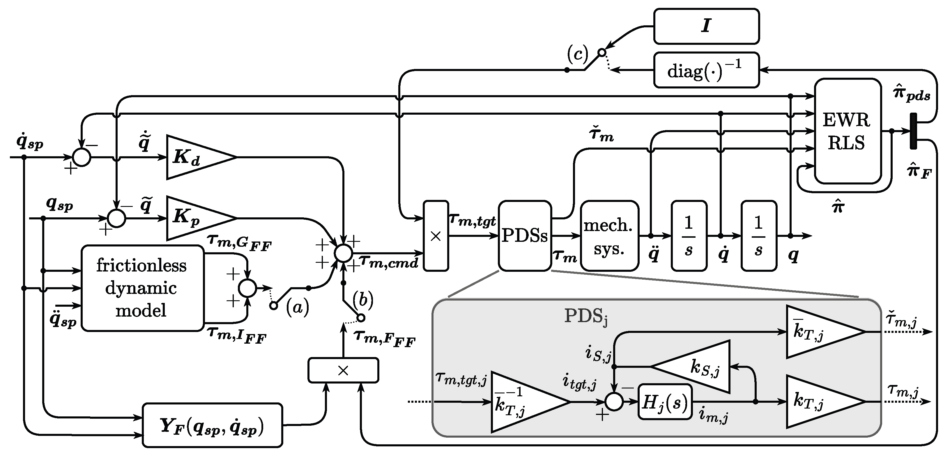
• A pure Proportional Derivative (PD) feedback controller (switch $\left(c\right)$ closed and $\left(a\right)$ and $\left(b\right)$ open);
• A Computed Torque Controller (CTC) in which the frictionless dynamics are accounted for by the a priori model (switches $\left(c\right)$ and $\left(a\right)$ closed and $\left(b\right)$ open);
• An Adaptive Controller (AC) in which the results of the friction identification framework are also inserted (switches $\left(a\right)$, $\left(b\right)$, and $\left(c\right)$ closed).

This kind of comparison, as will be shown in the following discussion, enables the quantification of the dynamic performance improvements (in terms of tracking and positioning errors) that can be obtained first from the introduction of the frictionless dynamic feedforward contribution only, and then from the further addition of the adaptive friction compensation. As will be experimentally demonstrated, a significant improvement can be obtained thanks to the information extracted from the adaptive dynamic model described above.

3. Results and Discussion

3.1. Case Study Description

5R Robot Model

Figure 2a depicts the 5R manipulator that was selected to experimentally validate the proposed methods, highlighting both the five-bar linkage and the position of the IMUs; Figure 2b, on the other hand, reports the kinematic scheme of the robot, whose main geometric parameters are the lengths of the proximal and distal links ($l_{p,1}$, $l_{p,2}$, $l_{d,1}$, and $l_{d,2}$, respectively) and the length $l_f$ of the fixed link. The main reference system, whose origin is denoted as $\mathit{o}$, is also displayed in the figure. The notable angular quantities are the actuated joint angles $q_1$ and $q_2$; the angles ${\phi }_1$ and ${\phi }_2$ between the distal links and the global x axis; and the five internal angles ${\psi }_j$, which coincide with the relative angular displacements between connected links. Finally, the positions of the revolute joints (denoted as ${\mathit{s}}_{\mathbf{1}}$, ${\mathit{s}}_{\mathbf{2}}$${\mathit{e}}_{\mathbf{1}}$, ${\mathit{e}}_{\mathbf{2}}$, and $\mathit{p}$) and of the centres of mass ${\mathit{c}}_{\mathit{p},\mathbf{1}}$, ${\mathit{c}}_{\mathit{p},\mathbf{2}}$, ${\mathit{c}}_{\mathit{d},\mathbf{1}}$, and ${\mathit{c}}_{\mathit{d},\mathbf{2}}$ of each link are also shown, together with the offset vectors ${\mathit{r}}_{\mathit{p},\mathbf{1}}\left(q_1\right)=({\mathit{c}}_{\mathit{p},\mathbf{1}}-{\mathit{s}}_{\mathbf{1}})$, ${\mathit{r}}_{\mathit{p},\mathbf{2}}\left(q_2\right)=({\mathit{c}}_{\mathit{p},\mathbf{2}}-{\mathit{s}}_{\mathbf{2}})$, ${\mathit{r}}_{\mathit{d},\mathbf{1}}\left({\phi }_1\right)=({\mathit{c}}_{\mathit{d},\mathbf{1}}-{\mathit{e}}_{\mathbf{1}})$, and ${\mathit{r}}_{\mathit{d},\mathbf{2}}\left({\phi }_2\right)=({\mathit{c}}_{\mathit{d},\mathbf{2}}-{\mathit{e}}_{\mathbf{2}})$. A numerical quantification for the main geometric parameters described above is reported in

Table 1. Geometric parameters of the robot; all quantities in $\left[\mathrm{m}\mathrm{m}\right]$.

${\mathit{l}}_{\mathit{f}}$	${\mathit{l}}_{\mathit{p},1}$	${\mathit{l}}_{\mathit{p},2}$	${\mathit{l}}_{\mathit{d},1}$	${\mathit{l}}_{\mathit{d},2}$	${\mathit{r}}_{\mathit{p},1}{|}_{{\mathit{q}}_1=0}$	${\mathit{r}}_{\mathit{p},2}{|}_{{\mathit{q}}_2=0}$	${\mathit{r}}_{\mathit{d},1}{|}_{{\mathit{\phi }}_1=0}$	${\mathit{r}}_{\mathit{d},2}{|}_{{\mathit{\phi }}_2=0}$
180	250	250	250	250	${\left[118.8,-0.7\right]}^{\top }$	${\left[118.8,-0.7\right]}^{\top }$	${\left[125.4,-0.9\right]}^{\top }$	${\left[130.3,0.6\right]}^{\top }$

.

The kinematics of this mechanism is well known and exactly solvable. Given the actuated joint angles $\mathit{q}$, points ${\mathit{e}}_{\mathbf{1}}$ and ${\mathit{e}}_{\mathbf{2}}$ can, in particular, be written as follows:

$$\begin{array}{cc}\hfill {\mathit{e}}_{\mathbf{1}}& ={\left[\begin{array}{cc}{l}_{p,1}cos\left(q_1\right)-l_f/2& l_{p,1}sin\left(q_1\right)\end{array}\right]}^{\top }\hfill \end{array}$$

(24)

$$\begin{array}{cc}\hfill {\mathit{e}}_{\mathbf{2}}& ={\left[\begin{array}{cc}{l}_{p,2}cos\left(q_2\right)+l_f/2& l_{p,2}sin\left(q_2\right)\end{array}\right]}^{\top }.\hfill \end{array}$$

(25)

The position $\mathit{p}$ can be found by solving the following system of equations:

$$\begin{array}{c}\hfill {p_1}^2+e_{1,1}^2-2e_{1,1}{p}_1+{p_2}^2+e_{1,2}^2-2e_{1,2}{p}_2=l_{d,1}^2\end{array}$$

(26)

$$\begin{array}{c}\hfill {p_1}^2+e_{2,1}^2-2e_{2,1}{p}_1+{p_2}^2+e_{2,2}^2-2e_{2,2}{p}_2=l_{d,2}^2\end{array}$$

(27)

which allows for, in general, up to two solutions, of which the one displaying the greater value associated with $p_2$ is selected in practice. Concerning, on the other hand, the inverse position kinematics, given $\mathit{p}$, the point ${\mathit{e}}_{\mathit{j}}$ (with $j\in \{1,2\}$) can be found by solving the following system:

$$\begin{array}{cc}\hfill & e_{j,1}^2+p_1^2-2p_1{e}_{j,1}+e_{j,2}^2+p_2^2-2p_2{e}_{j,2}=l_{d,j}^2\hfill \end{array}$$

(28)

$$\begin{array}{cc}\hfill & e_{j,1}^2+s_{j,1}^2-2s_{j,1}{e}_{j,1}+e_{j,2}^2+s_{j,2}^2-2s_{j,2}{e}_{j,2}=l_{p,j}^2;\hfill \end{array}$$

(29)

For this specific case study, due to otherwise occurring mechanical interferences, the solution characterized by the lowest value for $e_{1,1}$ and the highest value for $e_{2,1}$ is always preferred. The angles $q_1$, $q_2$, ${\phi }_1$, and ${\phi }_2$ measured from the global x axis are as follows:

$$\begin{array}{cc}\hfill q_j& =arctan\left({\displaystyle \frac{e_{j,2}-s_{j,2}}{e_{j,1}-s_{j,1}}}\right)\forall j\in \{1,2\}\hfill \end{array}$$

(30)

$$\begin{array}{cc}\hfill {\phi }_j& =arctan\left({\displaystyle \frac{p_2-e_{j,2}}{p_1-e_{j,1}}}\right)\forall j\in \{1,2\},\hfill \end{array}$$

(31)

whereas the internal angles ${\psi }_j$ may be trivially computed as ${\psi }_1=q_1$, ${\psi }_2=\pi -q_2$, ${\psi }_3=\pi -{\phi }_2+q_2$, ${\psi }_4={\phi }_2-{\phi }_1$, and ${\psi }_5=\pi -q_1+{\phi }_1$.

Keeping in mind that the Jacobian matrices associated with ${\mathit{e}}_{\mathbf{1}}$ and ${\mathit{e}}_{\mathbf{2}}$ and their partial derivatives are

$${\mathit{D}}_{{\mathit{e}}_{\mathbf{1}}}=l_{p,1}\left[\begin{array}{cc}-sin\left(q_1\right)& 0\\ cos\left(q_1\right)& 0\end{array}\right],{\displaystyle \frac{\partial {\mathit{D}}_{{\mathit{e}}_{\mathbf{1}}}}{\partial q_1}}=l_{p,1}\left[\begin{array}{cc}-cos\left(q_1\right)& 0\\ -sin\left(q_1\right)& 0\end{array}\right],{\displaystyle \frac{\partial {\mathit{D}}_{{\mathit{e}}_{\mathbf{1}}}}{\partial q_2}}=\left[\begin{array}{cc}0& 0\\ 0& 0\end{array}\right],$$

(32)

$${\mathit{D}}_{{\mathit{e}}_{\mathbf{2}}}=l_{p,2}\left[\begin{array}{cc}0& -sin\left(q_2\right)\\ 0& cos\left(q_2\right)\end{array}\right],{\displaystyle \frac{\partial {\mathit{D}}_{{\mathit{e}}_{\mathbf{2}}}}{\partial q_1}}=\left[\begin{array}{cc}0& 0\\ 0& 0\end{array}\right],{\displaystyle \frac{\partial {\mathit{D}}_{{\mathit{e}}_{\mathbf{2}}}}{\partial q_2}}=l_{p,2}\left[\begin{array}{cc}0,& -cos\left(q_2\right)\\ 0,& -sin\left(q_2\right)\end{array}\right],$$

(33)

the Jacobian analysis of the mechanism may be performed through the side-by-side differentiation of Equations (26) and (27) by $q_1$ and $q_2$, which, with simple rearrangements, leads to a system of equations each with the following form:

$$\begin{array}{c}\hfill {\displaystyle \sum _{h=1}^2}(p_h-e_{i,h})\left({\displaystyle \frac{\partial p_h}{\partial q_j}}-{\displaystyle \frac{\partial e_{i,h}}{\partial q_j}}\right)=0\end{array}$$

(34)

for all $(i,j)\in \{1,2\}\times \{1,2\}$. These four linear equations yield the four unknown partial derivatives of $p_1$ and $p_2$, which can then be rearranged in the Jacobian matrix ${\mathit{D}}_{\mathit{p}}$. A second-order differentiation of Equation (34) may analogously yield the partial derivatives of ${\mathit{D}}_{\mathit{p}}$ with respect to $q_1$ and $q_2$ through the solution of a system of linear equations each with the following form:

$$\begin{array}{c}\hfill {\displaystyle \sum _{h=1}^2}(p_h-e_{i,h})\left({\displaystyle \frac{{\partial }^2{p}_h}{\partial q_j\partial q_k}}-{\displaystyle \frac{{\partial }^2{e}_{i,h}}{\partial q_j\partial q_k}}\right)+\left({\displaystyle \frac{\partial p_h}{\partial q_j}}-{\displaystyle \frac{\partial e_{i,h}}{\partial q_j}}\right)\left({\displaystyle \frac{\partial p_h}{\partial q_k}}-{\displaystyle \frac{\partial e_{i,h}}{\partial q_k}}\right)=0,\end{array}$$

(35)

for all $(i,j,k)\in \{1,2\}\times \{1,2\}\times \{1,2\}$. The partial derivatives of ${\phi }_1$ and ${\phi }_2$ with respect to $q_1$ and $q_2$ are, on the other hand, characterized by the following expression:

$$\begin{array}{c}\hfill {\displaystyle \frac{\partial {\phi }_i}{\partial q_j}}={\displaystyle \frac{1}{l_{d,i}^2}}\left((p_1-e_{i,1})\left({\displaystyle \frac{\partial p_2}{\partial q_j}}-{\displaystyle \frac{\partial e_{i,2}}{\partial q_j}}\right)-(p_2-e_{i,2})\left({\displaystyle \frac{\partial p_1}{\partial q_j}}-{\displaystyle \frac{\partial e_{i,1}}{\partial q_j}}\right)\right)\end{array}$$

(36)

for all $(i,j)\in \{1,2\}\times \{1,2\}$. Further derivation yields

$$\begin{array}{c}\hfill \begin{array}{cc}\hfill {\displaystyle \frac{{\partial }^2{\phi }_i}{\partial q_j\partial q_k}}={\displaystyle \frac{1}{l_{d,i}^2}}(& (p_1-e_{i,1})\left({\displaystyle \frac{{\partial }^2{p}_2}{\partial q_j\partial q_k}}-{\displaystyle \frac{{\partial }^2{e}_{i,2}}{\partial q_j\partial q_k}}\right)-(p_2-e_{i,2})\left({\displaystyle \frac{{\partial }^2{p}_1}{\partial q_j\partial q_k}}-{\displaystyle \frac{{\partial }^2{e}_{i,1}}{\partial q_j\partial q_k}}\right)+\hfill \\ \hfill & \left({\displaystyle \frac{\partial p_1}{\partial q_j}}-{\displaystyle \frac{\partial e_{i,1}}{\partial q_j}}\right)\left({\displaystyle \frac{\partial p_2}{\partial q_k}}-{\displaystyle \frac{\partial e_{i,2}}{\partial q_k}}\right)-\left({\displaystyle \frac{\partial p_2}{\partial q_j}}-{\displaystyle \frac{\partial e_{i,2}}{\partial q_j}}\right)\left({\displaystyle \frac{\partial p_1}{\partial q_k}}-{\displaystyle \frac{\partial e_{i,1}}{\partial q_k}}\right)),\hfill \end{array}\end{array}$$

(37)

for all $(i,j,k)\in \{1,2\}\times \{1,2\}\times \{1,2\}$. Given Equation (36), it is important to immediately arrange the first-order partial derivatives into Jacobian matrices ${\mathit{D}}_{{\phi }_1}$, ${\mathit{D}}_{{\phi }_2}$ and also to compute the Jacobians ${\mathit{D}}_{{\psi }_j}$ of the relative angles. Also, the second-order derivatives obtained from Equation (37) might be arranged as required in a matrix form. The finite and differential kinematics of the centres of mass of the several links are then easily derived using the standard formulas that describe rigid-body motions. The finite and differential kinematics of the proximal links’ centres of mass are very easily obtained, as they simply undergo pure rotation around the grounded revolute joints. Concerning, on the other hand, the point ${\mathit{c}}_{\mathit{d},\mathit{i}}$, its position may be expressed as follows:

$$\begin{array}{c}\hfill {\mathit{c}}_{\mathit{d},\mathit{i}}={\mathit{e}}_{\mathit{i}}+\mathit{A}\left({\phi }_i\right){\mathit{r}}_{\mathit{d},\mathit{i}}{|}_{{\phi }_i=0},\end{array}$$

(38)

in which

$$\begin{array}{c}\hfill \mathit{A}\left({\phi }_i\right)=\left[\begin{array}{cc}cos\left({\phi }_i\right)& -sin\left({\phi }_i\right)\\ sin\left({\phi }_i\right)& cos\left({\phi }_i\right)\end{array}\right].\end{array}$$

(39)

After differentiating Equation (38) once and then twice, the following relationships are obtained:

$$\begin{array}{cc}\hfill {\displaystyle \frac{\partial {\mathit{c}}_{\mathit{d},\mathit{i}}}{\partial q_j}}& ={\displaystyle \frac{\partial {\mathit{e}}_{\mathit{i}}}{\partial q_j}}+{\displaystyle \frac{\partial {\phi }_i}{\partial q_j}}{\displaystyle \frac{\partial \mathit{A}\left({\phi }_i\right)}{\partial {\phi }_i}}{\mathit{r}}_{\mathit{d},\mathit{i}}{|}_{{\phi }_i=0}\hfill \end{array}$$

(40)

$$\begin{array}{cc}\hfill {\displaystyle \frac{{\partial }^2{\mathit{c}}_{\mathit{d},\mathit{i}}}{\partial q_j\partial q_k}}& ={\displaystyle \frac{{\partial }^2{\mathit{e}}_{\mathit{i}}}{\partial q_j\partial q_k}}+\left({\displaystyle \frac{{\partial }^2{\phi }_i}{\partial q_j\partial q_k}}{\displaystyle \frac{\partial \mathit{A}\left({\phi }_i\right)}{\partial {\phi }_i}}+{\displaystyle \frac{\partial {\phi }_i}{\partial q_j}}{\displaystyle \frac{\partial {\phi }_i}{\partial q_k}}{\displaystyle \frac{{\partial }^2\mathit{A}\left({\phi }_i\right)}{\partial {{\phi }_i}^2}}\right){\mathit{r}}_{\mathit{d},\mathit{i}}{|}_{{\phi }_i=0}.\hfill \end{array}$$

(41)

Concerning the statics of this particular mechanism, it may be noted that it is constrained to move in the horizontal plane; therefore, the Lagrangian components associated with the gravitational forces are null and will not be considered further in the following discussion. On the other hand, given the above kinematic analysis and a quantification of the mass and inertial parameters of the mechanical elements, it is rather straightforward to determine the matrices $\mathit{M}$ and $\mathit{C}$ that characterize the system’s dynamics. In particular, defining the vector $\mathit{\chi }$ as

$$\begin{array}{c}\hfill \mathit{\chi }={\left[\begin{array}{c}{q}_1,q_2,{\phi }_1,{\phi }_2,c_{d,1,1},c_{d,1,2},c_{d,2,1},c_{d,2,2},p_1,p_2\end{array}\right]}^{\top }\end{array}$$

(42)

the Jacobian matrix ${\mathit{D}}_{\mathit{\chi }}$ and its partial derivatives are obtained from the concatenation of the already calculated derivatives, while the total derivative with respect to time is as follows:

$$\begin{array}{c}\hfill {\dot{\mathit{D}}}_{\mathit{\chi }}={\displaystyle \sum _{j=1}^2}{\displaystyle \frac{\partial {\mathit{D}}_{\mathit{\chi }}}{\partial q_j}}{\dot{q}}_j.\end{array}$$

(43)

Then, the constant matrix ${\mathit{M}}^{*}$ is defined as

$$\begin{array}{c}\hfill {\mathit{M}}^{*}=\mathrm{diag}\left(\left[\begin{array}{c}{I}_{p,1},I_{p,2},I_{d,1},I_{d,2},m_{d,1},m_{d,1},m_{d,2},m_{d,2},m_p,m_p\end{array}\right]\right),\end{array}$$

(44)

in which $m_p$ is the mass concentrated in $\mathit{p}$, and $m_{d,1}$, $m_{d,2}$, $I_{d,1}$, and $I_{d,2}$ are the masses and the barycentric inertias of the distal links. Finally, the quantities $I_{p,1}$ and $I_{p,2}$ indicate the proximal links’ inertias computed with respect to the points ${\mathit{s}}_{\mathbf{1}}$ and ${\mathit{s}}_{\mathbf{2}}$, which are also inclusive of the inertial contributions of the motors, the gearboxes, and the masses concentrated in ${\mathit{e}}_{\mathbf{1}}$ and ${\mathit{e}}_{\mathbf{2}}$. The values of these mass and inertial parameters, as obtained from the solid model of the robot, are reported in

Table 2. Mass and inertial parameters of the robot.

${\mathit{I}}_{\mathit{p},1}$, [kg m2]	${\mathit{I}}_{\mathit{p},2}$, [kg m2]	${\mathit{I}}_{\mathit{d},1}$, [kg m2]	${\mathit{I}}_{\mathit{d},2}$, [kg m2]	${\mathit{m}}_{\mathit{d},1}$, [kg]	${\mathit{m}}_{\mathit{d},2}$, [kg]	${\mathit{m}}_{\mathit{p}},$ [kg]
0.292	0.292	0.030	0.036	2.32	2.78	2.72

.

The matrices $\mathit{M}$ and $\mathit{C}$ are obtained as follows:

$$\begin{array}{c}\hfill \mathit{M}={\mathit{D}}_{\mathit{\chi }}^{\top }{\mathit{M}}^{*}{\mathit{D}}_{\mathit{\chi }}\end{array}$$

(45)

$$\begin{array}{c}\hfill \mathit{C}={\mathit{D}}_{\mathit{\chi }}^{\top }{\mathit{M}}^{*}{\dot{\mathit{D}}}_{\mathit{\chi }}.\end{array}$$

(46)

Finally, the Lagrangian components associated with the motor torques ${\mathit{\tau }}_{\mathit{m}}$ may be simply computed as ${\mathit{Q}}_{\mathit{m}}=\mathrm{diag}\left([{\iota }_1,{\iota }_2]\right){\mathit{\tau }}_{\mathit{m}}$, with ${\iota }_1$ and ${\iota }_2$ being the reduction ratios of the gearboxes.

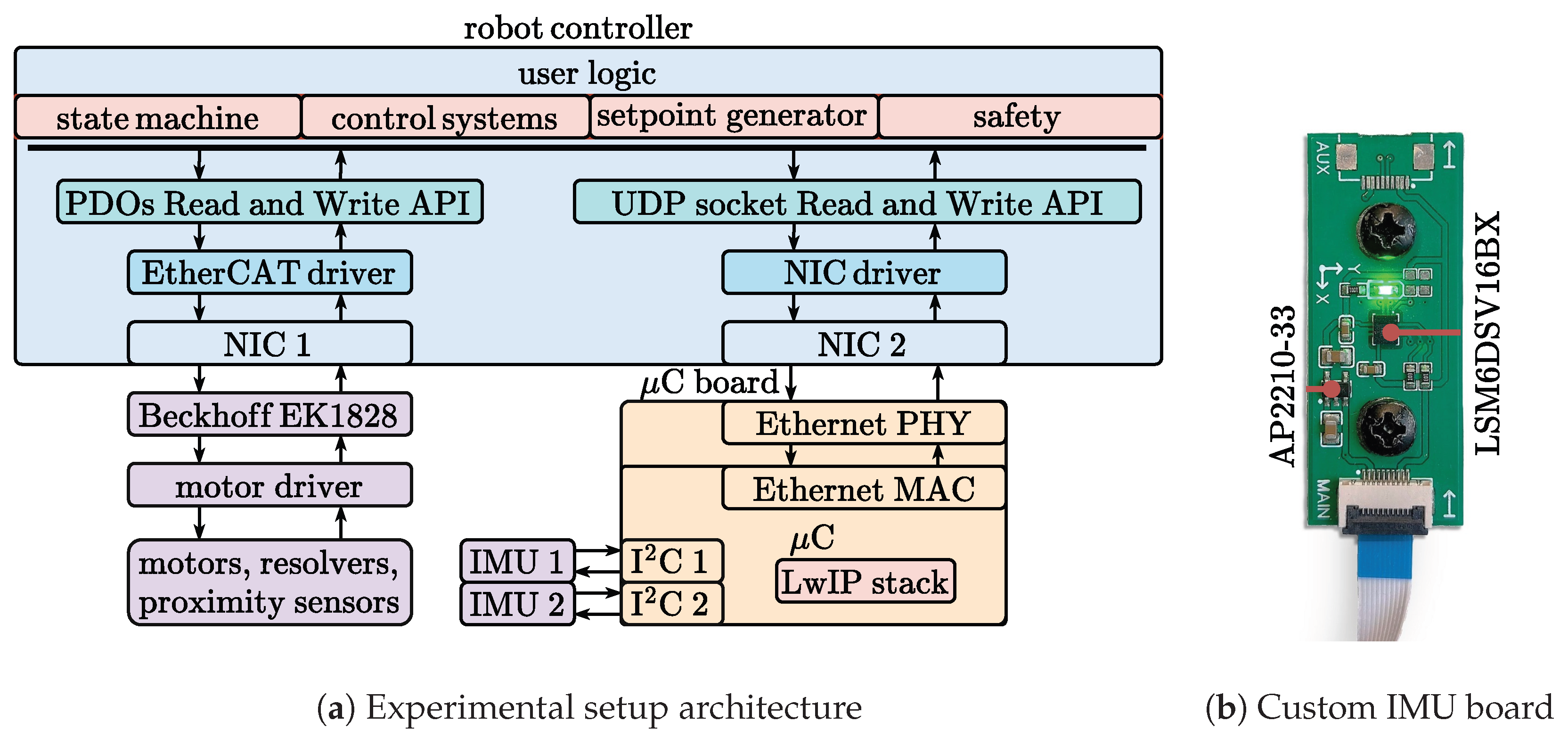
3.2. Experimental Setup

Figure 3a reports a scheme of the developed software and hardware architecture. In particular, the main hardware elements that compose the experimental setup are as follows:

• A desktop equipped with two Network Interface Cards (NICs) and serving as the robot controller;
• A Beckhoff EK1828 EtherCAT head;
• A Copley Control Accelnet BE2-090-20-R dual-axis motor driver operating in torque mode and acting as an EtherCAT subordinate device;
• Two Mavilor BLS55 Brushless AC motors whose resolvers are used by the driver to generate virtualized rotary encoder signals;
• Two proximity sensors used in the zeroing phase;
• An STM32 F439ZI microcontroller (μC) capable of Ethernet connectivity and equipped with two I²C interfaces set to Fast Mode operation;
• Two ST LSM6DSV16BX triaxial IMUs with an integrated I²C interface, each mounted on the custom board depicted in Figure 3b; the other notable component mounted on the PCB is the AP2210-33 voltage regulator, which was selected due to its high power supply rejection ratio.

The robot controller runs the Simulink Real-Time (2017a) OS, which supports a native EtherCAT main device driver, at a base frequency of $f_s=4$ kHz; the UDP communication with the μC happens at a lower frequency $f_{UDP}$, equal to 1 kHz. All computations, including the evaluation of the robot’s dynamic model for the inertial feedforward and each EWR-RWS iteration, are executed at the base frequency within the temporal deadline set by the sample time $T_s=0.25$ ms, where the required data provided by the IMUs are oversampled. The internal sample rate of the accelerometers and gyroscopes was set to 7.68 kHz in the high-performance mode; the accelerometers have a full scale set to ±2 g, and the gyroscopes are set to ±1000 deg/s. The current setup makes use of only a single axis for each MEMS sensor; in particular, due to the mounting configuration, only the z axis of the gyroscopes and the y axis of the accelerometers are used to measure, respectively, the angular velocity and the tangential acceleration of the links. The acceleration is further converted into an angular acceleration through a scaling factor equal to the inverse of the distance between the accelerometer and the grounded revolute joint; this distance was selected in order to reasonably exploit the accelerometer’s full scale without exceeding it, considering the likely accelerations achievable by the manipulator. Mounting inaccuracies were compensated for through a simple calibration procedure: in particular, the gyroscope angular velocity measures were matched with the angular velocity obtained from the numerical differentiation of the encoder signals; analogously, the accelerometer signal was matched with the angular acceleration acquired from the numerical differentiation of the gyroscope signal.

The matching was performed with scale factors ${\alpha }_{g,j}$ and ${\alpha }_{a,j}$ (with $j=1,2$) determined through least square regressions of the following form:

$$\begin{array}{cc}\hfill {\alpha }_{g,j}& ={\left({\dot{\mathit{q}}}_{\mathit{gz},\mathit{j}}^{\top }{\dot{\mathit{q}}}_{\mathit{gz},\mathit{j}}\right)}^{-1}{\dot{\mathit{q}}}_{\mathit{gz},\mathit{j}}^{\top }{\dot{\mathit{q}}}_{\mathit{e},\mathit{j}},\hfill \end{array}$$

(47)

$$\begin{array}{cc}\hfill {\alpha }_{a,j}& ={\left({\mathit{a}}_{\mathit{y},\mathit{j}}^{\top }{\mathit{a}}_{\mathit{y},\mathit{j}}\right)}^{-1}{\mathit{a}}_{\mathit{y},\mathit{j}}^{\top }{\alpha }_{g,j}{\ddot{\mathit{q}}}_{\mathit{gz},\mathit{j}}.\hfill \end{array}$$

(48)

In Equation (47), ${\dot{\mathit{q}}}_{\mathit{gz},\mathit{j}}$ is a vector of raw measures provided by the z-channel of the $j^{th}$ gyroscope, and ${\dot{\mathit{q}}}_{\mathit{e},\mathit{j}}$ is a vector (of the same size) of angular velocities obtained from the numerical differentiation of the corresponding encoder count. In Equation (48), ${\mathit{a}}_{\mathit{y},\mathit{j}}$ represents a vector of raw acceleration measures provided by the $j^{th}$ accelerometer y-channel; ${\ddot{\mathit{q}}}_{\mathit{gz},\mathit{j}}$ is the vector obtained from the numerical differentiation of the raw gyroscope signal. Care was taken to obtain ${\dot{\mathit{q}}}_{\mathit{gz},\mathit{j}}$ and ${\mathit{a}}_{\mathit{y},\mathit{j}}$ in motion conditions that spanned the relevant ranges of velocities and accelerations.

In a more general application, in which the links can rotate and translate in the three-dimensional space, it would be necessary, first of all, to account for the effect of gravity on the accelerometers’ measures; moreover, if the accelerometer is installed, e.g., on a serial manipulator on a link different from the first one, its reading must be depurated from the motion determined by the previous joints. In general terms, then, the kinematic model of the robot should be used in order to obtain a measure of $\dot{\mathit{q}}$ and $\ddot{\mathit{q}}$ from the velocity and acceleration vectors provided by the IMUs.

Concerning, finally, the trajectories used to test the proposed methods, these are not specially crafted for identification purposes; rather, they are random, high-speed point-to-point motions planned as joint-space straight segments that cover a large portion of the useful workspace of the robot. This kind of trajectory, a few of which are exemplified in Figure 4, simulates realistic pick-and-place operations on scattered targets. In particular, Figure 4a provides a joint-space representation of the condition index $\sigma =\sqrt{{\mu }_{min}/{\mu }_{max}}$ (obtained from the eigenvalues ${\mu }_{min}$ and ${\mu }_{max}$ of ${\mathit{D}}_{\mathit{p}}^{\top }{\mathit{D}}_{\mathit{p}}$ and plotted in the red colour scale); the well-conditioned convex polygon in which the manipulator motions are planned (drawn in black); and four consecutive trajectories, with the blue colour scale indicating the velocity. From Figure 4b, which represents the same quantities in the task space, it may be appreciated that the peak velocities at the tool centre point $\mathit{p}$ are in excess of 1 m s⁻¹; these high speeds result in motions that last, end-to-end, a maximum of 0.82 s (considering the longest possible one). The configuration parameters for the considered trajectories are constituted by the lower and upper bounds for joint velocities (${\dot{q}}_{j,lb}$ and ${\dot{q}}_{j,ub}$), accelerations (${\ddot{q}}_{j,lb}$ and ${\ddot{q}}_{j,ub}$), and motion jerk (${\stackrel{⃛}{q}}_{j,lb}$ and ${\stackrel{⃛}{q}}_{j,ub}$); these values are all reported in

Table 3. Trajectory configuration parameters.

${\dot{\mathit{q}}}_{\mathit{j},\mathit{ub}}\left[\frac{\mathrm{deg}}{s}\right]$	${\dot{\mathit{q}}}_{\mathit{j},\mathit{lb}}\left[\frac{\mathrm{deg}}{s}\right]$	${\ddot{\mathit{q}}}_{\mathit{j},\mathit{ub}}\left[\frac{\mathrm{deg}}{s^2}\right]$	${\ddot{\mathit{q}}}_{\mathit{j},\mathit{lb}}\left[\frac{\mathrm{deg}}{s^2}\right]$	${\stackrel{⃛}{\mathit{q}}}_{\mathit{j},\mathit{ub}}\left[\frac{\mathrm{deg}}{s^3}\right]$	${\stackrel{⃛}{\mathit{q}}}_{\mathit{j},\mathit{lb}}\left[\frac{\mathrm{deg}}{s^3}\right]$
210	$-210$	1680	$-1680$	25,200	−25,200

.

These upper and lower bounds constrain an optimization algorithm that generates piecewise jerk-continuous motion laws according to Pontryagin’s optimality principle; as a result, the trajectories have, at each instant, the maximum or minimum admissible value or a null jerk value; accelerations and velocities are such that the bounds are not violated and trajectory execution times are minimized. It should be noted that the experimental results presented in the following discussion do not concern a single trajectory, but rather a large number of them, all generated randomly according to the algorithm briefly described above.

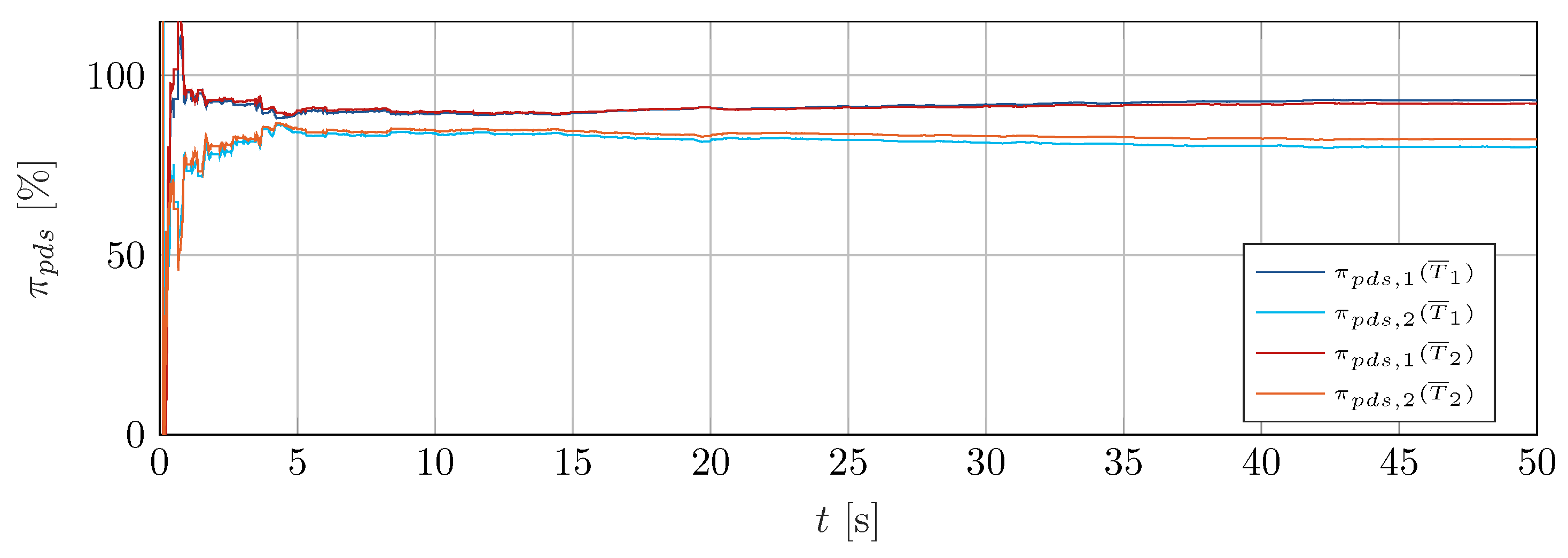
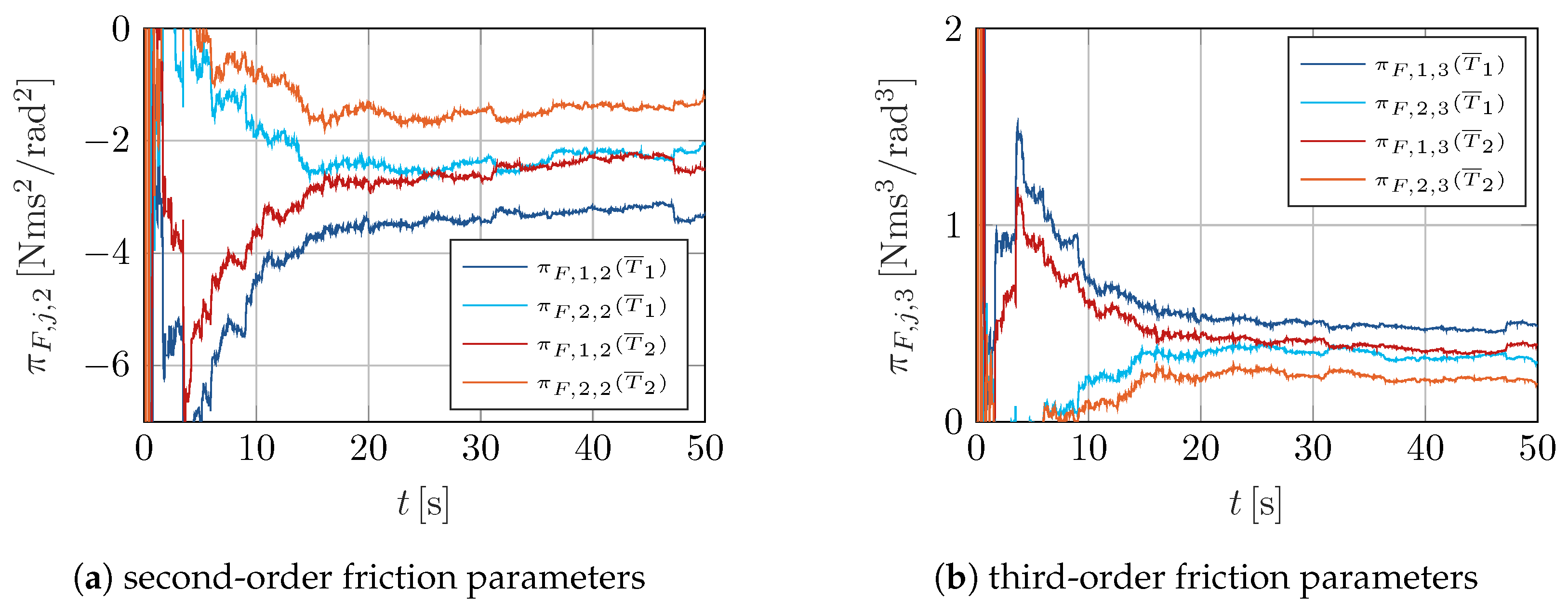
3.3. Experimental Results

The proposed friction model is, in general, suitable for the identification of the parameters of all joints, but through the appropriate removal of rows from ${\mathit{\pi }}_{\mathit{F}}$ and corresponding columns from ${\mathit{Y}}_{\mathit{F}}$, it can be simplified to fit those cases in which some of the joints have negligible contributions to the overall frictional Lagrangian components ${\mathit{Q}}_{\mathit{F}}$. In order to select the most appropriate polynomial order and to check for the presence of almost frictionless joints, the friction model variants listed and described in

Table 4. Friction model configurations.

	Model $\left(1\right)$	Model $\left(2\right)$	Model $\left(3\right)$	Model $\left(4\right)$	Model $\left(5\right)$
considered joints	all	active only	active only	active only	active only
polynomial order	4	4	3	2	1

were defined at the outset of the experimental activities.

The first, model $\left(1\right)$, is of the fourth order and inclusive of all revolute joints; the remaining four consider just the active joints and are, respectively, of the fourth, third, second, and first polynomial order. Over the course of an initial test, each model was used in an open loop, with its RMS estimation residual

$$\begin{array}{c}\hfill {\rho }_{rms}\left(t\right)=\sqrt{{\displaystyle \frac{1}{t}}{\int }_0^t{(Y_{\sum }\left(u\right)\mathit{\pi }\left(u\right)-R_{\sum }\left(u\right))}^2\mathrm{d}u}\end{array}$$

(49)

being recorded over the course of the experiment.

Figure 5 reports the results of this preliminary investigation and thus enables a comparison between the friction model variants. In the figure, it may be observed that, even though model $\left(1\right)$, the most complex, is indeed the best performing, models $\left(2\right)$ and $\left(3\right)$ come very close to it in terms of predictive performance, with the advantage of having a greatly reduced number of parameters. A more significant gap is observable between models $\left(3\right)$ and $\left(4\right)$, and a larger gap still exists between models $\left(4\right)$ and $\left(5\right)$. These results show that, consistent with the presence of gearboxes, friction torques arising in the actuated joints are markedly dominant over those related to the passive hinges. In practice, therefore, the dynamic behaviour of the system may be well explained considering only the former and neglecting the latter. Furthermore, a third-order polynomial appears to be the most appropriate one, as further increases lead to abruptly diminishing returns in terms of fitting accuracy.

This quantitative analysis leads to the conclusion that, for this specific setup, a third-order model considering only the active joints is the most appropriate one. Henceforth, the following discussion will therefore concern the results obtained with model (3). For clarity of exposition, it should be remarked that its parameters are ordered and named as follows:

$$\begin{array}{c}\hfill {\mathit{\pi }}_{\left(\mathbf{3}\right)}={[{\pi }_{pds,1},{\pi }_{pds,2},{\pi }_{F,1,0},{\pi }_{F,1,1},{\pi }_{F,1,2},{\pi }_{F,1,3},{\pi }_{F,2,0},{\pi }_{F,2,1},{\pi }_{F,2,2},{\pi }_{F,2,3}]}^{\top },\end{array}$$

(50)

with ${\pi }_{pds,j}$ having the obvious meaning, and ${\pi }_{F,j,0}$, ${\pi }_{F,j,1}$, ${\pi }_{F,j,2}$, and ${\pi }_{F,j,3}$ each indicating the zero-, first-, second-, and third-order frictional parameter of actuated joint j.

Figure 6a depicts, in blue, for grounded joint 1, the relationship between the velocity and friction Lagrangian components at room temperature; Figure 6b reports the same quantities for grounded joint 2. The depicted data points were obtained considering the steady-state value ${\overline{\widehat{\mathit{\pi }}}}_{\mathit{pds}}$ of ${\widehat{\mathit{\pi }}}_{\mathit{pds}}$ (which, as shown in the following discussion, converges robustly), the indirectly measured motor torque, and the frictionless dynamics model, according to the following equation:

$$\begin{array}{c}\hfill {\mathit{Q}}_{\mathit{F}}={\mathit{Y}}_{\mathit{pds}}(\mathit{q},{\check{\mathit{\tau }}}_{\mathit{m}}){\overline{\widehat{\mathit{\pi }}}}_{\mathit{pds}}-{\mathit{Q}}_{\mathit{I}}(\mathit{q},\dot{\mathit{q}},\ddot{\mathit{q}}).\end{array}$$

(51)

The gravitational component ${\mathit{Q}}_{\mathit{G}}$ is not considered in Equation (51) because, as already introduced, it is null for this particular mechanism. No other kind of processing or filtering, other than a downsampling to 200 Hz for logging purposes, was adopted for these data, nor for those presented in the following discussion.

The red points, on the other hand, represent the friction component predicted by the model; the observable dispersion is due to the fact that the friction parameters are not constant, but rather are allowed to change in time. A good fit is obtained especially for angular velocities under 2 rad s⁻¹, with the stiction regime not affecting the estimation of the static friction parameters. As the velocity increases, the torque data are increasingly scattered, but also, in these conditions, the model appears to remain broadly unbiased.

The quality of the fitting is also apparent in the time domain, as might be seen in Figure 7a,b. These figures report, for each actuator, the actually provided motor torque Lagrangian components ${\mathit{Q}}_{\mathit{m}}=-{\mathit{Y}}_{\mathit{pds}}(\mathit{q},{\check{\mathit{\tau }}}_{\mathit{m}}){\overline{\widehat{\mathit{\pi }}}}_{\mathit{pds}}$ (calculated taking into account the steady-state value ${\overline{\widehat{\mathit{\pi }}}}_{\mathit{pds}}$) and the associated predictions stemming from the a priori frictionless dynamics model and from the estimated friction model. The figures depict the overall Lagrangian components, and hence, their vertical scales are wider than those of Figure 6a,b. This is the first factor that makes the data dispersion less apparent, though it may also still be seen here, especially in the time intervals included between the torque peaks, where velocities are high. The second reason is related to the different time intervals: whereas the panels of Figure 7 cover a 10 $\mathrm{s}$ span, the data displayed in Figure 6 were collected along a 55 $\mathrm{s}$ run.

As already noted, both the frictionless dynamics and the friction models are not used for mere prediction, but rather, they constitute important components that augment the PD feedback action; in particular, as previously remarked, the addition of the frictionless dynamic contribution yields the CTC, while the further introduction of the friction feedforward component leads to the AC. Indeed, this work is focused on the enhancement of the dynamic performances of the system, chiefly measured by the achieved position errors. Figure 8 and Figure 9 report, in particular, the peak and RMS joint position errors ${\tilde{\mathit{q}}}_{\mathit{peak}}$ and ${\tilde{\mathit{q}}}_{\mathit{rms}}$ for the three controllers operating in otherwise identical conditions, over the course of pseudo-random (and reseeded) trajectories spanning forty seconds. It should be remarked that, in this time frame, several tens of trajectories are executed, considering that, as already mentioned, the longest (in spatial and temporal terms) one lasts only slightly more than $0.8$ $\mathrm{s}$.

It may be observed that, although the inertial feedforward contribution alone is capable of markedly reducing the peak and RMS errors compared to the PD controller, further significant benefits are obtained thanks to the estimated friction model. In particular, the effect of friction feedforward is especially evident on the RMS errors. These aggregate results may also be clearly seen in the time domain, as attested by Figure 10, which, for visual clarity reasons, does not cover the entire 40 $\mathrm{s}$ span, but nevertheless, it still reports ten randomized trajectories.

In particular, the top panels report the joint acceleration (Figure 10a), velocity (Figure 10b), and position setpoints (Figure 10c) as a function of time. The three bottom panels show, on the other hand, the joint errors achieved on these desired trajectories for the three controllers; it may be remarked that the vertical axis scales are different in order to best represent the shape and features of the error profiles.

Indeed, when simultaneously observing Figure 10a,d, it can be seen that, for the PD controller, the error peaks occur at the acceleration and deceleration phases of the motions; these peaks are effectively removed thanks to the frictionless dynamic feedforward mechanism introduced by the CTC, as seen in Figure 10e, where, however, some errors associated with the high-velocity portion of the trajectories (cf. Figure 10b) remain. Moreover, at the beginning of each trajectory, a steep change in the error’s value, attributable to static friction, occurs; for the same reason, each trajectory terminates with a non-null error. Finally, in Figure 10f, it may be observed that the velocity-related errors are further reduced by the friction feedforward term; in particular, the effects of friction, both in the stiction and in the sliding regimes, are in large part compensated.

Considering the AC, Figure 11 highlights the relative weight, in RMS terms, of the three torque components.

In particular, the dynamic feedforward accounts for 45% and 48% of the torques exerted by motor 1 and 2. The friction feedforward contributions amount, on the other hand, to 40% and 33%. The quantitative importance of the friction torques is even more striking when considering the highly dynamic nature of the executed trajectories, during which significant inertial actions are to be expected; clearly, the relevance of friction would stand out even more in applications characterized by slower movements. The relative weight of the feedback contribution at motor 2 falls short of 20%; at motor 1, an even lower 15% is achieved. This leads to the conclusion that the feedforward components are broadly capable of generating the desired motion, with rather minor feedback corrections being required. These are clearly still needed, not least to compensate the fluctuations in friction torques, which, as already discussed, present a certain dispersion around the value predicted by the adaptive model. All the results presented so far concern situations in which an adequate estimation of the unknown parameters has been achieved. Questions concerning the robustness and speed of convergence remain to be addressed, considering that several endogenous (e.g., wear) and exogenous factors may affect friction and its identification. A significant influence is exerted by temperature in particular; this is attested by Figure 12a,b, which show, respectively, for grounded joint 1 and 2, a general lowering of the friction actions with increasing temperature. This work is not focused on the definition of the exact causal mechanisms behind this observable trend, which, in general, is driven by complex factors such as changes in lubricant viscosity and film thickness and clearances between mechanical parts. On the other hand, given that changes due to temperature do occur, it is important to verify that the proposed estimation algorithm is able to track them.

The data presented in the figure were collected as follows: The machine was turned on after a pause long enough to achieve thermal equilibrium with the surrounding environment, taking care to measure the external temperature of the two gearboxes, which, on average, was found to be equal to ${\overline{T}}_1=22$ °C. A first acquisition was then performed for 150 s, which yielded the data represented in blue. Subsequently, the robot was brought to a new thermal equilibrium through the repeated execution of high-speed alternate and symmetric motions for a total duration of 120 min, after which an average of ${\overline{T}}_2=39$ °C was recorded. This value is representative of both gearboxes’ states, as the temperature difference between the two was less than 2 °C. A second acquisition, also lasting 150 s, finally provided the data reported in red. The temperature measures were performed with two type K thermocouples each attached to the gearbox casings and read by two AM-520-EUR digital multimeters.

Figure 13, Figure 14 and Figure 15 report on the other time history of the estimated parameters, considering the two aforementioned thermal conditions and the same initialization of parameters. It should be stressed that the adopted initial values, namely ${\widehat{\mathit{\pi }}}_{\mathit{pds}}\left(t_0\right)=\mathbf{1}$ and ${\widehat{\mathit{\pi }}}_{\mathit{F}}\left(t_0\right)=\mathbf{0}$, correspond to those that might be assigned in the absence of any prior information or data and thus constitute a worst-case scenario when testing the convergence properties of the proposed method. In a more realistic use case, previous estimates might be saved together with the internal state of the EWR-RLS estimator to assign better initial guesses and to further speed up the convergence.

From Figure 13, it may be seen, in particular, that the PDS parameters are not strongly affected by temperature. Their value moreover reaches convergence in less than 5 s.

The results reported in Figure 14 concern the friction parameters of zero (Figure 14a) and first orders (Figure 14b); their convergence appears to be slightly slower, as their value reaches a roughly stationary level after around 15 s. As anticipated, the identification process results in different estimates for the parameters’ values depending on the considered joint (despite the fact that they are nominally identical to each other) and on the temperature. The latter indeed has the effect of lowering the estimated friction parameters.

A similar picture emerges from Figure 15b, which concerns the cubic friction parameters. The quadratic parameters depicted in Figure 15a, are negative and decrease with the temperature in absolute value. These results are consistent with the data presented in Figure 12.

In general, this experimental analysis confirms that the convergence of the parameters is quick, even considering an unfavourable initialization, and in particular, orders of magnitude faster than the changes due to temperature; the suitability of the adaptive mechanism to operate in non-stationary, slowly changing conditions is thus confirmed.

4. Conclusions

The paper proposed a general method for real-time friction identification in robotic and mechatronic devices, with a focus on dynamic performance enhancement; the theoretical, implementative, and applicative aspects are all covered in the discussion. In particular, the method proposes the use of MEMS IMUs comprising triaxial accelerometers and gyroscopes to measure the linear accelerations and angular velocities of the manipulator’s links in order to obtain the information needed to adaptively estimate joint friction concurrently to the system’s normal functioning. The proposed method is applicable not only to serial robots but also to parallel kinematic manipulators or more, in general, to any kind of machinery in which relative motions between rigid bodies give rise to friction. The requirements for the application of the method are an accurate estimation of the moving masses, which nowadays can be easily obtained from the engineering tools used to model the device’s mechanical components; an appropriate kinematic analysis of the relative motions; the selection of a suitable friction model; and the ability to measure the actual motions up to the accelerations, with MEMS sensors currently constituting an interesting possibility due to their increasing performance and modest cost. Within the context of the current engineering landscape, the assumption of known masses does not constitute a limitation, but rather an opportunity to investigate the usually neglected effects of tolerances and inaccuracies introduced by the power drive systems. In fact, using the accurate frictionless dynamic model of the mechanism as ground truth, it is possible to identify and subsequently compensate not only friction forces and torques, but also the unwanted gains introduced by the electric driver and motor pairs. Beyond the theoretical exposition, the method was experimentally validated in all its hardware and software components using a 5R PKR as a case study. The wide-ranging experimental activities demonstrated not only the method’s ability to predict friction torques but also the sizeable benefits obtained in terms of tracking error reduction when closed-loop operation is activated. In particular, compared to a simple PD controller, the addition of the frictionless dynamics feedforward component reduced the RMS joint position errors, on a sample of tens of trajectories, by a factor of 2.44 on the first joint and 2.04 on the second. The peak errors were similarly reduced by factors of 3.88 and 3.78. The addition of the adaptive friction compensation further reduced the RMS errors by another factor of 5.05 and 3.68 on each joint; the peak errors were also, again, reduced by factors of 1.40 and 1.97.

A powerful feature of the proposed methodology is its adaptability to non-stationary conditions, even though a simple velocity-based friction model is used. In particular, given the short convergence time (around 10 $\mathrm{s}$ for the fitting residual even in the absence of a good first guess for the friction parameters), there is scarcely any need to parametrize the model with respect to, for example, temperature, since the resulting variations in friction loads can be tracked by the real-time estimation algorithm. This opens up, as potential areas of research, further applications such as monitoring, diagnostics, and predictive maintenance based on anomalous changes in friction actions. More immediately, straightforward applications to other robotic and mechatronic systems where unknown friction actions should be tracked and compensated for to increase the control performance may follow. Another planned activity concerns the experimental comparison between the IMU-based adaptive method proposed here and similar algorithms that do not require such sensors to better highlight the foreseeable advantages of direct velocity and acceleration measurements over indirect observation. Future refinements of the proposed method, finally, may include variable payload estimation, automatic model complexity reduction, and the introduction of redundant IMUs to obtain more reliable measures through sensor fusion techniques.

References

1. Righettini, P.; Strada, R.; Cortinovis, F. General Procedure for Servo-Axis Design in Multi-Degree-of-Freedom Machinery Subject to Mixed Loads. Machines 2022, 10, 454. [Google Scholar] [CrossRef]
2. Righettini, P.; Strada, R.; Cortinovis, F. Neural Network Mapping of Industrial Robots’ Task Times for Real-Time Process Optimization. Robotics 2023, 12, 143. [Google Scholar] [CrossRef]
3. Righettini, P.; Strada, R.; Cortinovis, F. Experimental Evaluation of Centralized Control Strategies on a 5R Robot. Mech. Mach. Sci. 2024, 163 MMS, 334–342. [Google Scholar] [CrossRef]
4. Righettini, P.; Strada, R.; Cortinovis, F.; Tabaldi, F.; Santinelli, J.; Ginammi, A. An Experimental Investigation of the Dynamic Performances of a High Speed 4-DOF 5R Parallel Robot Using Inverse Dynamics Control. Robotics 2024, 13, 54. [Google Scholar] [CrossRef]
5. Márton, L.; Van Der Linden, F. Temperature dependent friction estimation: Application to lubricant health monitoring. Mechatronics 2012, 22, 1078–1084. [Google Scholar] [CrossRef]
6. Liu, H.; Liu, H.; Zhu, C.; Parker, R. Effects of lubrication on gear performance: A review. Mech. Mach. Theory 2020, 145, 103701. [Google Scholar] [CrossRef]
7. Lontin, K.; Khan, M. Interdependence of friction, wear, and noise: A review. Friction 2021, 9, 1319–1345. [Google Scholar] [CrossRef]
8. Al-Bender, F.; De Moerlooze, K. Characterization and modeling of friction and wear: An overview. Int. J. Sustain. Constr. Des. 2011, 2, 19–28. [Google Scholar] [CrossRef]
9. Kato, K. Wear in relation to friction - A review. Wear 2000, 241, 151–157. [Google Scholar] [CrossRef]
10. Zhang, T.; Chen, X.; Gu, J.; Wang, Z. Influences of preload on the friction and wear properties of high-speed instrument angular contact ball bearings. Chin. J. Aeronaut. 2018, 31, 597–607. [Google Scholar] [CrossRef]
11. Farhat, N.; Mata, V.; Page, A.; Daz-Rodríguez, M. Dynamic simulation of a parallel robot: Coulomb friction and stick-slip in robot joints. Robotica 2010, 28, 35–45. [Google Scholar] [CrossRef]
12. Hao, L.; Pagani, R.; Beschi, M.; Legnani, G. Dynamic and friction parameters of an industrial robot: Identification, comparison and repetitiveness analysis. Robotics 2021, 10, 49. [Google Scholar] [CrossRef]
13. Luo, R.; Yuan, J.; Hu, Z.; Du, L.; Bao, S.; Zhou, M. Lie-theory-based dynamic model identification of serial robots considering nonlinear friction and optimal excitation trajectory. Robotica 2024, 42, 3552–3569. [Google Scholar] [CrossRef]
14. Karahan, O.; Karci, H. Swarm Intelligence Based Nonlinear Friction and Dynamic Parameters Identification for a 6-DOF Robotic Manipulator. J. Intell. Robot. Syst. Theory Appl. 2023, 108, 19. [Google Scholar] [CrossRef]
15. Chaoui, H.; Sicard, P.; Lakhsasr, A.; Schwartz, H. Neural network based model reference adaptive control structure for a flexible joint with hard nonlinearities. In Proceedings of the 2004 IEEE International Symposium on Industrial Electronics, Ajaccio, France, 4–7 May 2004; Volume 1, pp. 271–276. [Google Scholar] [CrossRef]
16. Chaoui, H.; Sicard, P.; Gueaieb, W. ANN-based adaptive control of robotic manipulators with friction and joint elasticity. IEEE Trans. Ind. Electron. 2009, 56, 3174–3187. [Google Scholar] [CrossRef]
17. de Wit, C.; Lischinsky, P.; Åström, K.; Olsson, H. A New Model for Control of Systems with Friction. IEEE Trans. Autom. Control 1995, 40, 419–425. [Google Scholar] [CrossRef]
18. de Wit, C.C.; Lischinsky, P. Adaptive Friction Compensation with Dynamic Friction Model. IFAC Proc. Vol. 1996, 29, 2078–2083. [Google Scholar] [CrossRef]
19. Azizi, Y.; Yazdizadeh, A. Passivity-based adaptive control of a 2-DOF serial robot manipulator with temperature dependent joint frictions. Int. J. Adapt. Control Signal Process. 2019, 33, 512–526. [Google Scholar] [CrossRef]
20. Piatkowski, T. Dahl and LuGre dynamic friction models - The analysis of selected properties. Mech. Mach. Theory 2014, 73, 91–100. [Google Scholar] [CrossRef]
21. Swevers, J.; Al-Bender, F.; Ganseman, C.; Prajogo, T. An integrated friction model structure with improved presliding behavior for accurate friction compensation. IEEE Trans. Autom. Control 2000, 45, 675–686. [Google Scholar] [CrossRef]
22. Lampaert, V.; Swevers, J.; Al-Bender, F. Modification of the Leuven integrated friction model structure. IEEE Trans. Autom. Control 2002, 47, 683–687. [Google Scholar] [CrossRef]
23. Liu, Y.; Li, J.; Zhang, Z.; Hu, X.; Zhang, W. Experimental comparison of five friction models on the same test-bed of the micro stick-slip motion system. Mech. Sci. 2015, 6, 15–28. [Google Scholar] [CrossRef]
24. Lampaert, V.; Swevers, J.; Al-Bender, F. Experimental comparison of different friction models for accurate low-velocity tracking. In Proceedings of the 2004 American Control Conference, Boston, MA, USA, 30 June–2 July 2002; pp. 1121–1126. [Google Scholar]
25. Sun, Y.H.; Chen, T.; Wu, C.; Shafai, C. Comparison of four friction models: Feature prediction. J. Comput. Nonlinear Dyn. 2016, 11, 031009. [Google Scholar] [CrossRef]
26. Slotine, J.J.E.; Li, W. On the adaptive control of robot manipulators. Int. J. Robot. Res. 1987, 6, 49–59. [Google Scholar] [CrossRef]
27. Slotine, J.J.; Li, W. Composite adaptive control of robot manipulators. Automatica 1989, 25, 509–519. [Google Scholar] [CrossRef]
28. Spong, M.; Ortega, R. On Adaptive Inverse Dynamics Control of Rigid Robots. IEEE Trans. Autom. Control 1990, 35, 92–95. [Google Scholar] [CrossRef]
29. Odry, A.; Fullér, R.; Rudas, I.; Odry, P. Kalman filter for mobile-robot attitude estimation: Novel optimized and adaptive solutions. Mech. Syst. Signal Process. 2018, 110, 569–589. [Google Scholar] [CrossRef]
30. Dai, F.; Gao, X.; Jiang, S.; Guo, W.; Liu, Y. A two-wheeled inverted pendulum robot with friction compensation. Mechatronics 2015, 30, 116–125. [Google Scholar] [CrossRef]
31. Pei, Y.; Kleeman, L. Mobile robot floor classification using motor current and accelerometer measurements. In Proceedings of the 2016 IEEE 14th International Workshop on Advanced Motion Control (AMC), Auckland, New Zealand, 22–24 April 2016; pp. 545–552. [Google Scholar] [CrossRef]
32. Pang, G.; Liu, H. Evaluation of a low-cost MEMS accelerometer for distance measurement. J. Intell. Robot. Syst. Theory Appl. 2001, 30, 249–265. [Google Scholar] [CrossRef]
33. Georgy, J.; Karamat, T.; Iqbal, U.; Noureldin, A. Enhanced MEMS-IMU/odometer/GPS integration using mixture particle filter. GPS Solut. 2011, 15, 239–252. [Google Scholar] [CrossRef]
34. Kada, B.; Munawar, K.; Shaikh, M.; Hussaini, M.; Al-Saggaf, U. UAV Attitude Estimation Using Nonlinear Filtering and Low-Cost Mems Sensors. IFAC-PapersOnLine 2016, 49, 521–528. [Google Scholar] [CrossRef]
35. Euston, M.; Coote, P.; Mahony, R.; Kim, J.; Hamel, T. A complementary filter for attitude estimation of a fixed-wing UAV. In Proceedings of the 2008 IEEE/RSJ International Conference on Intelligent Robots and Systems, Nice, France, 22–26 September 2008; pp. 340–345. [Google Scholar] [CrossRef]
36. Min, F.; Wang, G.; Liu, N. Collision detection and identification on robot manipulators based on vibration analysis. Sensors 2019, 19, 1080. [Google Scholar] [CrossRef]
37. Pucher, F.; Gattringer, H.; Müller, A. Collision detection for flexible link robots using accelerometers. IFAC-PapersOnLine 2019, 52, 514–519. [Google Scholar] [CrossRef]
38. Birjandi, S.; Fortunic, E.; Haddadin, S. Evaluation of Robot Manipulator Link Velocity and Acceleration Observer. IFAC-PapersOnLine 2023, 56, 292–299. [Google Scholar] [CrossRef]
39. Xu, T.; Fan, J.; Fang, Q.; Wang, S.; Zhu, Y.; Zhao, J. A novel virtual sensor for estimating robot joint total friction based on total momentum. Appl. Sci. 2019, 9, 3344. [Google Scholar] [CrossRef]
40. Jin, M.; Kang, S.; Chang, P. Robust compliant motion control of robot with nonlinear friction using time-delay estimation. IEEE Trans. Ind. Electron. 2008, 55, 258–269. [Google Scholar] [CrossRef]
41. Kou, B.; Huang, Y.; Wang, P.; Ren, D.; Zhang, J.; Guo, S. A New Parameter Identification Method for Industrial Robots with Friction. Machines 2022, 10, 349. [Google Scholar] [CrossRef]
42. Roveda, L.; Bussolan, A.; Braghin, F.; Piga, D. Robot joint friction compensation learning enhanced by 6D virtual sensor. Int. J. Robust Nonlinear Control 2022, 32, 5741–5763. [Google Scholar] [CrossRef]
43. Tadese, M.; Yumbla, F.; Yi, J.S.; Lee, W.; Park, J.; Moon, H. Passivity Guaranteed Dynamic Friction Model with Temperature and Load Correction: Modeling and Compensation for Collaborative Industrial Robot. IEEE Access 2021, 9, 71210–71221. [Google Scholar] [CrossRef]
44. Nevmerzhitskiy, M.; Notkin, B.; Vara, A.; Zmeu, K. Friction Model of Industrial Robot Joint with Temperature Correction by Example of KUKA KR10. J. Robot. 2019, 2019, 6931563. [Google Scholar] [CrossRef]
45. Afrough, M.; Hanieh, A. Identification of Dynamic Parameters and Friction Coefficients: Of a Robot with Planar Serial Kinemtic Linkage. J. Intell. Robot. Syst. Theory Appl. 2019, 94, 3–13. [Google Scholar] [CrossRef]
46. Liu, S.; Wang, L.; Wang, X. Sensorless force estimation for industrial robots using disturbance observer and neural learning of friction approximation. Robot.-Comput.-Integr. Manuf. 2021, 71, 102168. [Google Scholar] [CrossRef]
47. Khishtan, A.; Kim, S.; Lee, J. A hybrid model in a nonlinear disturbance observer for improving compliance error compensation of robotic machining. Robot. -Comput.-Integr. Manuf. 2025, 92, 102887. [Google Scholar] [CrossRef]
48. Chen, C.; Zhang, W.; Liu, T.; Zhang, Z.; Lu, W.; Wang, L.; Zheng, Y.; Lin, Z. Online identification of inertial parameters of a robot with partially combined links using IMU sensing. Mechatronics 2023, 94, 103023. [Google Scholar] [CrossRef]
49. Patel, A.; Ferdowsi, M. Current sensing for automotive electronics - A survey. IEEE Trans. Veh. Technol. 2009, 58, 4108–4119. [Google Scholar] [CrossRef]
50. Renner, A.; Wind, H.; Sawodny, O. Online payload estimation for hydraulically actuated manipulators. Mechatronics 2020, 66, 102322. [Google Scholar] [CrossRef]
51. Cochrane, C.; Lenahan, P. Real time exponentially weighted recursive least squares adaptive signal averaging for enhancing the sensitivity of continuous wave magnetic resonance. J. Magn. Reson. 2008, 195, 17–22. [Google Scholar] [CrossRef]
Figure 1. Adaptive control scheme.
Robotics 14 00036 g001
Figure 2. (a) Top view of the manipulator; (b) kinematic scheme.
Robotics 14 00036 g002
Figure 3. Software and hardware architecture of the experimental setup (a); developed IMU board with its main components (b).
Robotics 14 00036 g003
Figure 4. Robot workspace and selected trajectories executed during the experimental tests; representations in the joint-space (a) and in the task-space (b).
Robotics 14 00036 g004
Figure 5. Fitting residuals for friction models of decreasing complexity.
Robotics 14 00036 g005
Figure 6. Friction Lagrangian components on actuated joints 1 and 2: inferred from measurement and frictionless dynamics model in blue; estimated through the friction model in red.
Robotics 14 00036 g006
Figure 7. Motor torque Lagrangian component for actuated joints 1 and 2; experimental data in blue, prediction in red.
Robotics 14 00036 g007
Figure 8. Peak joint position errors for the three tested controllers.
Robotics 14 00036 g008
Figure 9. RMS joint position errors for the three tested controllers.
Robotics 14 00036 g009
Figure 10. Setpoints and joint position errors for the three controllers.
Robotics 14 00036 g010
Figure 11. RMS feedback and feedforward torque contributions as a percentage of the total.
Robotics 14 00036 g011
Figure 12. Temperature effects on friction torque data for actuated joints 1 and 2: low-temperature data in blue; high-temperature data in red.
Robotics 14 00036 g012
Figure 13. Convergence of the PDS parameters at different temperatures.
Robotics 14 00036 g013
Figure 14. Temperature effects on the zero- and first-order friction parameters.
Robotics 14 00036 g014
Figure 15. Temperature effects on the second and third order friction parameters.
Robotics 14 00036 g015