Inverse and Forward Kinematics and CAD-Based Simulation of a 5-DOF Delta-Type Parallel Robot with Actuation Redundancy

Abstract

This article introduces a novel modification of a Delta-type parallel robot. The robot has five degrees of freedom and provides its end-effector with a 3T2R motion pattern (three translational and two rotational degrees of freedom). The fifth degree of freedom (rotation) is kinematically decoupled from the other four motions, and it is controlled by two drives. Thus, the proposed robot has a redundant actuation. In this article, we present an algorithm to solve the inverse kinematics of this robot and apply it to a path modeling example of a spiral-like trajectory. Numerical simulations illustrate the algorithm and show how the actuated coordinates change along the considered trajectory. Forward kinematics follows next, and an approach is introduced to determine all end-effector configurations for the specified displacements in the actuated joints. A numerical example presents four assembly modes of the robot corresponding to four real solutions of the forward kinematic problem. Finally, this article demonstrates a computer-aided design and analysis of the proposed robot: we describe a procedure for analyzing inverse kinematics and calculating actuation torques. This study forms the basis for the future manufacturing and experimental analysis of a robot prototype.

1. Introduction

The Delta robot, proposed by Clavel [1] in the 1980s, has become one of the most commercially and technologically successful parallel robots. This robot can have either rotational or linear drives. In the latter case, carriages, driven by a ball screw or belt drive, move along linear guides, which usually have a horizontal, vertical, or inclined orientation [2]. The inclined axes of the actuated joints were also used in Delta-type robots with rotational drives. An example of such a robot is NUWAR [3]. The inclined axes provided this robot with greater workspace dimensions compared with the original model [1]. Papers [4,5] present other Delta-type robots with inclined axes.

With its simple design and high-performance capabilities, the Delta robot is attractive to numerous researchers and has served as a prototype for various mechanisms and devices, including Linapod [6], the H4 robot [7], Orthoglide [8], the I4 robot [9], the Eureka robot [10], Delta Keops [2], the Par4 robot [11], the Heli4 robot [12], and Delthaptic [13]. Although the Delta robot was initially proposed for high-speed pick-and-place operations, mechanisms with identical or similar structures have found application in other industries, such as machining [14], medicine [15], additive technologies [16], and high-precision operations [17].

The Delta-type robots discussed above differ in terms of their design and degrees of freedom (DOF), determined by their practical realization. Actuation redundancy is another feature of Delta-type robots that can improve their performance. In this case, a robot has extra actuated kinematic chains or extra actuators added to its passive joints [18]. In [19], the authors examined the advantages of actuation redundancy in parallel mechanisms. These advantages include the exclusion or avoidance of singular configurations, homogeneous and symmetric force output, stiffness improvement within the workspace, and the opportunity to use low-powered drives. Additionally, redundantly actuated systems remain controllable even if one or more actuators break down.

At the same time, few studies have considered the actuation redundancy in Delta-type robots. One example is the Eureka robot [10] with three translational and two rotational DOF (a 3T2R motion pattern) controlled by six drives. It could reach a $\pm {90}^{\circ }$ rotation about one axis and a complete rotation about another axis. In [20], the authors applied an optimal redundancy coordination method to another redundantly actuated parallel mechanism. It relied on a 3-DOF Delta robot coupled with an additional 1-DOF parallel mechanism, where every kinematic chain was a slider-crank linkage. This system provided redundant actuation to the vertical translation. Paper [21] used actuation redundancy to obtain high accelerations in Delta-type robots with 3T and 3T1R motion patterns. High accelerations are critical for rapid pick-and-place operations, the primary application of Delta-type robots. In that study, actuation redundancy was achieved by adding similar actuated kinematic chains. Paper [22] introduced a haptic device called DELTA-R (formerly known as DELTA-4). Unlike the classical Delta robot [1], it included two kinematic chains, each with two drives. Four drives controlled three DOF of the end-effector. Other redundantly actuated 3-DOF Delta-type robots were studied in [23]. They had symmetric (Sym-RAL DELTA) and asymmetric (Asym-RAL DELTA) structures with horizontal linear guides, which supported four kinematic chains with driving carriages. These designs enlarged the workspace by singularity-free mode changes. Paper [24] showed a 3-DOF robot, where every kinematic chain had an additional actuated link. Six drives controlled three translational DOF of the end-effector. This structure provided the robot with reconfigurability that enlarged its workspace. The authors of [25] considered a Delta-type robot with a 3T1R motion pattern. It included six actuated kinematic chains with linear guides, where two chains used parallelogram linkages. The robot end-effector rotated for more than ${90}^{\circ }$.

The review above showed that redundantly actuated Delta-type robots generally had three DOF (a 3T motion pattern) or four DOF (a 3T1R motion pattern). We have found only one model with another mobility, equal to five (the Eureka robot). On the other hand, the additional DOF can significantly extend the practical applications of such systems. In this regard, we propose a new 5-DOF Delta-type robot with actuation redundancy. The major contributions of this paper include developing the kinematic algorithms for this novel robot, which provide closed-form solutions to both the inverse and forward kinematic problems. In addition, we present a computer-aided design (CAD) model of the robot and perform dynamic simulations using CAD tools.

The rest of this article has the following structure. Section 2 describes the design of the proposed robot. Section 3 and Section 4 consider its inverse and forward kinematics, respectively. Section 5 presents a computer model of the robot and solves the inverse dynamic problem using CAD software. Section 6 discusses the obtained results and proposed algorithms. Section 7 recaps the paper and mentions directions for future studies.

2. Robot Design

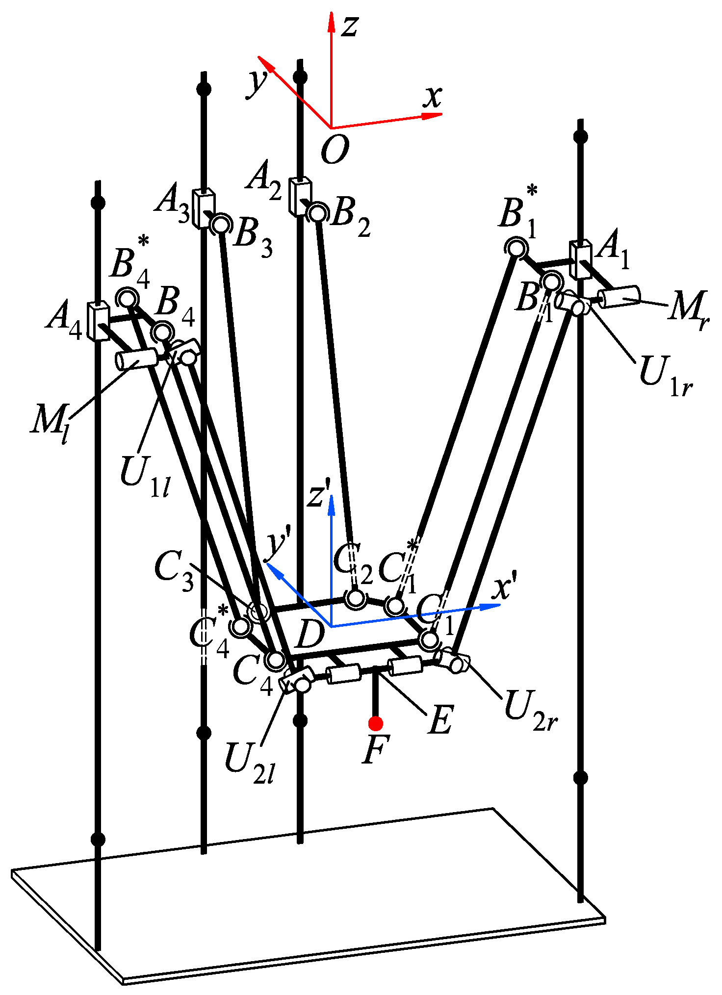
Figure 1 depicts the considered robot. It has four kinematic chains (branches) of two different types. Let $i=1,\dots ,4$ be an index number of a branch. Each branch connects to the base with carriage $A_i$, which translates vertically. In branches 1 and 4, the carriage is followed by parallelogram $B_i{B}_i^{*}{C}_i^{*}{C}_i$ with spherical joints in its vertices. One (shorter) side of this parallelogram is rigidly connected to the carriage, while the opposite side is connected to the moving plate. Branches 2 and 3 utilize single rod $B_i{C}_i$ with two spherical joints on their ends instead of a parallelogram. Branches 1 and 4 also include auxiliary drives (motors) $M_r$ and $M_l$, respectively. 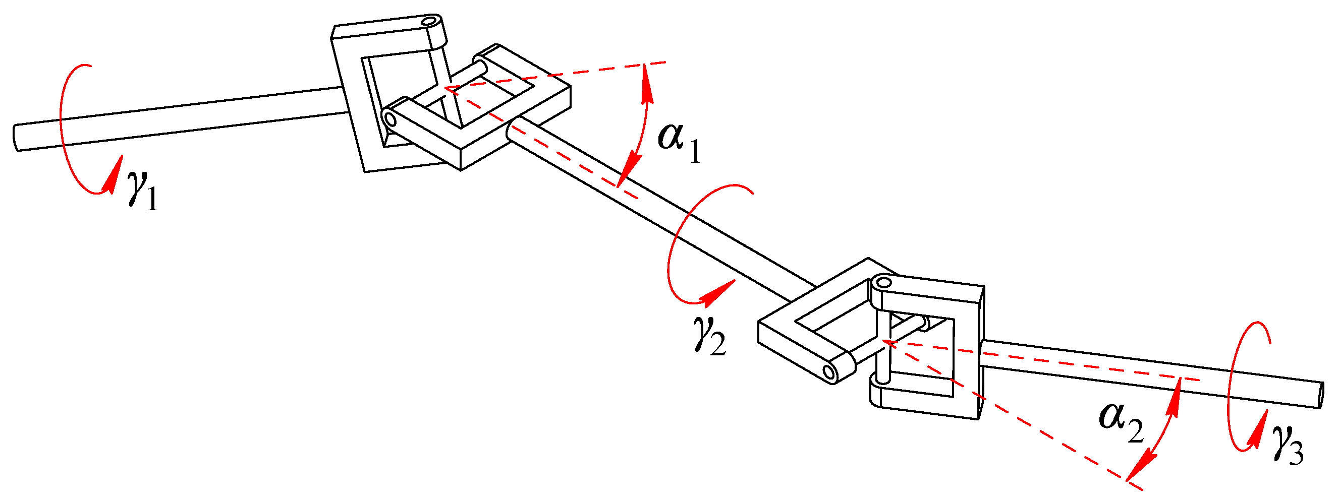These motors are connected to the tilt axis of the end-effector (tool) $EF$ with pairs of universal joints $U_{1r}$, $U_{2r}$ and $U_{1l}$, $U_{2l}$, respectively.

The robot design provides its end-effector with five degrees of freedom: three translations and two rotations. This motion pattern can be verified by looking at the constraints imposed by the branches. Branch 1 imposes two constraints on the moving plate, permitting three translational motions and only one rotation around the axis parallel to the shorter side of the parallelogram. Since branch 4 is placed directly opposite branch 1, it provides the same constraints. Branches 2 and 3 do not constrain the motion of the moving plate. Therefore, the moving plate of the robot has four DOFs (a more detailed and formal explanation based on the screw theory can be found in paper [26]). The second rotation (around the $U_{2r}{U}_{2l}$ axis) is kinematically decoupled from the four above-mentioned motions. Any external load (torque) corresponding to this DOF is resisted only by the motor that performs this rotation. To compensate for this drawback and distribute the load between two auxiliary branches, we use two motors—$M_r$ and $M_l$—which simultaneously control the rotation. Actuation redundancy also helps in situations in which one of the auxiliary branches is in a singular configuration (as discussed at the end of Section 3.1).

In the proposed design, the end-effector is attached to the moving plate by a revolute joint, and the plate forms a parallel mechanism with the base. Thus, the robot structure can be classified as a hybrid one. There are several Delta-type robots with a similar structure, for example, Eureka [10], Par4 [11], or Heli4 [12], where the end-effector also rotates relative to the moving plate. In these works, the authors considered their robots to be parallel. We follow the same convention and refer to the proposed robot as a parallel one.

This design is motivated by the outstanding performance of Delta-type robots, whose branches experience only the tensile loads. Therefore, expanding the capabilities of the Delta robot by introducing new rotational DOF is an interesting and relevant scientific problem. The proposed design can also be modified into a 6-DOF one by adding a central driving rod, like in the original Delta robot [1]. However, certain applications (e.g., machining) do not need the sixth DOF because it is realized by the rotation of the tool or the workpiece.

In the literature, we found only one similar Delta-type robot with redundant actuation. This is the Eureka robot designed by Krut et al. [10]. Its end-effector also has five DOF and a 3T2R motion pattern, but one rotational DOF differs from the robot we propose here. In Eureka, the tool rotates about its own axis and cannot tilt relative to the moving plate. As we discussed in the paragraph above, we often do not need this tool rotation because it can be provided by other means. Our design also does not use any additional transmission mechanisms, except for the two auxiliary branches—this is another advantage of the proposed robot. In contrast, Eureka does not have a solid moving plate and uses a rack and pinion transmission to achieve the end-effector rotation. This design increases the weight of the moving elements and worsens the robot positioning accuracy because of the inevitable backlash in the rack and pinion transmission. Thus, we believe the proposed robot has some advantages over Eureka and meets the concept of the light-weight Delta robot.

3. Inverse Kinematics

We start the kinematic analysis of the robot with its inverse kinematics. The inverse kinematic problem aims to compute actuated coordinates for a given configuration of the robot end-effector. This problem is essential for robot control because it allows the desired end-effector trajectory to be converted into the controlled motion of the actuators. In this section, we first present an algorithm to find a closed-from solution to the inverse kinematics, and then, we consider an example of a trajectory simulation using the proposed algorithm.

3.1. Solution Method

Let x, y, and z be the coordinates of the end-effector (point F) in stationary reference frame $Oxyz$, and ${\phi }_t$ and ${\phi }_p$ be the tilt angles of the tool and the moving plate, respectively. The goal of the inverse kinematics is to calculate position $h_i$ of each carriage and rotation angles ${\theta }_r$ and ${\theta }_l$ of both the right and left auxiliary drives (Figure 2).

Denoting a distance between points E and F as $l_{EF}$ and a distance between points D and E as $l_{DE}$, we first find coordinates $x_D$, $y_D$, and $z_D$ of point D:

$$\begin{array}{cc}\hfill x_D& =x+l_{EF}cos\left({\phi }_t\right)sin\left({\phi }_p\right),\hfill \\ \hfill y_D& =y-l_{EF}sin\left({\phi }_t\right)+l_{DE},\hfill \\ \hfill z_D& =z+l_{EF}cos\left({\phi }_t\right)cos\left({\phi }_p\right).\hfill \end{array}$$

(1)

Then, we compute coordinates $x_{Ci}$, $y_{Ci}$, and $z_{Ci}$ of point $C_i$:

$$\left[\begin{array}{c}{x}_{Ci}\\ y_{Ci}\\ z_{Ci}\end{array}\right]=\left[\begin{array}{c}{x}_D\\ y_D\\ z_D\end{array}\right]+\left[\begin{array}{ccc}cos\left({\phi }_p\right)& 0& sin\left({\phi }_p\right)\\ 0& 1& 0\\ -sin\left({\phi }_p\right)& 0& cos\left({\phi }_p\right)\end{array}\right]\left[\begin{array}{c}{x}_{Ci}^{\prime }\\ y_{Ci}^{\prime }\\ z_{Ci}^{\prime },\end{array}\right],$$

(2)

where $x_{Ci}^{\prime }$, $y_{Ci}^{\prime }$, and $z_{Ci}^{\prime }$ are the coordinates of point $C_i$ in moving reference frame $D{x}^{\prime }{y}^{\prime }{z}^{\prime }$.

A distance between points $B_i$ and $C_i$ remains constant, therefore:

$$l_{BiCi}^2={(x_{Ci}-x_{Bi})}^2+{(y_{Ci}-y_{Bi})}^2+{(z_{Ci}-z_{Bi})}^2,$$

(3)

where $l_{BiCi}$ is the length of rod $B_i{C}_i$; $x_{Bi}$, $y_{Bi}$, and $z_{Bi}$ are the coordinates of point $B_i$.

One can see that $h_i=z_{Bi}$ and parameters $x_{Bi}$ and $y_{Bi}$ depend only on the robot geometry. Thus, the value of $h_i$ can be calculated as follows:

$$h_i=\pm \sqrt{l_{BiCi}^2-{(x_{Ci}-x_{Bi})}^2-{(y_{Ci}-y_{Bi})}^2}+z_{Ci}.$$

(4)

The next step is to find the rotation angles of the auxiliary drives. It is well-known that a single universal joint cannot maintain a constant angular speed of its output shaft if it is not collinear with the input shaft. Let $\alpha$ be an angle between the axes of the input and output shafts. Depending on the initial configuration of the universal joint, the relation between input rotation angle ${\gamma }_1$ and output rotation angle ${\gamma }_2$ can be expressed by the following equations [27] (ch. 1):

$$tan\left({\gamma }_1\right)=cos\left(\alpha \right)tan\left({\gamma }_2\right),$$

(5)

if the yoke input shaft is in the plane spanned by the input and output shafts, or

$$tan\left({\gamma }_1\right)={\displaystyle \frac{tan\left({\gamma }_2\right)}{cos\left(\alpha \right)}},$$

(6)

if the yoke input shaft is orthogonal to this plane (Figure 3).

When two consecutive universal joints are used to transmit a rotational motion via the intermediate shaft, the so-called “phasing” is used. Two universal joints are phased if the output shaft of the first yoke is coplanar with the input shaft of the second yoke (Figure 4).

In the arrangement shown in Figure 4, we can obtain the relation between input angle ${\gamma }_1$ and output angle ${\gamma }_3$ using Equations (5) and (6):

$$tan\left({\gamma }_1\right)=tan\left({\gamma }_3\right){\displaystyle \frac{cos\left({\alpha }_1\right)}{cos\left({\alpha }_2\right)}}.$$

(7)

This arrangement is widely used because it compensates for angular speed fluctuations when the input and the output shafts are parallel. Indeed, Equation (7) shows that ${\alpha }_1={\alpha }_2$ in this case, and ${\gamma }_1={\gamma }_3$.

The discussed robot has two auxiliary branches, each with two consecutive universal joints. In general, the input and output shafts of these branches will not be parallel. Equation (7) will not be convenient in this case because of the ambiguity that arises if $cos\left({\alpha }_2\right)=0$. Therefore, we will use non-phased joints in the auxiliary branches, for which the output shaft of the first yoke is orthogonal to the input shaft of the second yoke. Using the notations introduced in Figure 2 and applying Equation (5) twice, we can write:

$$tan\left({\theta }_r\right)=tan\left({\phi }_t\right)cos\left({\beta }_{1r}\right)cos\left({\beta }_{2r}\right),tan\left({\theta }_l\right)=tan\left({\phi }_t\right)cos\left({\beta }_{1l}\right)cos\left({\beta }_{2l}\right),$$

(8)

from where

$${\theta }_r={tan}^{-1}(tan\left({\phi }_t\right)cos\left({\beta }_{1r}\right)cos\left({\beta }_{2r}\right)),{\theta }_l={tan}^{-1}(tan\left({\phi }_t\right)cos\left({\beta }_{1l}\right)cos\left({\beta }_{2l}\right)),$$

(9)

where ${\beta }_{1r}$, ${\beta }_{1l}$, ${\beta }_{2r}$, and ${\beta }_{2l}$ are the angles between the shafts according to Figure 2.

Assuming that each rod of the auxiliary branches remains parallel to corresponding rod $B_i{C}_i$ and the tilt axis of the tool remains parallel to $C_1{C}_4$, we can compute angles ${\beta }_{1r}$, ${\beta }_{1l}$, ${\beta }_{2r}$, and ${\beta }_{2l}$ as follows:

$$\begin{array}{cccc}\hfill {\beta }_{1r}& ={cos}^{-1}\left(\right|{\widehat{\mathbf{s}}}_x·{\widehat{\mathbf{s}}}_{B1C1}\left|\right),\hfill & \hfill {\beta }_{2r}& ={cos}^{-1}\left(\right|{\widehat{\mathbf{s}}}_{C1C4}·{\widehat{\mathbf{s}}}_{B1C1}\left|\right),\hfill \\ \hfill {\beta }_{1l}& ={cos}^{-1}\left(\right|{\widehat{\mathbf{s}}}_x·{\widehat{\mathbf{s}}}_{B4C4}\left|\right),\hfill & \hfill {\beta }_{2l}& ={cos}^{-1}\left(\right|{\widehat{\mathbf{s}}}_{C1C4}·{\widehat{\mathbf{s}}}_{B4C4}\left|\right),\hfill \end{array}$$

(10)

where ${\widehat{\mathbf{s}}}_x$ is a unit vector parallel to the $Ox$ axis and ${\widehat{\mathbf{s}}}_{B1C1}$, ${\widehat{\mathbf{s}}}_{B4C4}$, and ${\widehat{\mathbf{s}}}_{C1C4}$ are unit vectors along the lines that connect the corresponding points.

We have found displacements in all the actuated joints for the given configuration of the end-effector. Although we resolved the ambiguity of Equation (7) by using the non-phased joints, a universal joint cannot transmit the rotation if the angle between the input and output shafts is equal to ${90}^{\circ }$. Therefore, if at least one of angles ${\beta }_{1r}$, ${\beta }_{1l}$, ${\beta }_{2r}$, and ${\beta }_{2l}$ is equal to ${90}^{\circ }$, the corresponding auxiliary branch will be in a singular configuration. The actuation redundancy preserves the controllability of the fifth DOF in this case. Even if one auxiliary branch is in the singular configuration, we can still transmit the rotation to the end-effector using the second branch. The fifth DOF will be uncontrollable only when both auxiliary chains are singular, which is not possible in the proposed design.

This concludes the inverse kinematic analysis. The next subsection considers an example of the inverse kinematics solution for a desired end-effector trajectory.

3.2. Numerical Example

As an example, we suppose the end-effector has to follow a conical spiral path defined by the following equations:

$$\begin{array}{cc}\hfill x& =x_0-q\delta cos\left(\delta \right),\hfill \\ \hfill y& =y_0-q\delta sin\left(\delta \right),\hfill \\ \hfill z& =z_0-r\delta ,\hfill \end{array}$$

(11)

where $x_0$, $y_0$, and $z_0$ are the coordinates of the starting point; q is a coefficient that regulates the expansion rate of the spiral; r is a coefficient that regulates the rate of a tool descent along the path; $\delta$ is a varying parameter that defines a point on the trajectory.

We consider the trajectory with the following parameters:

$$\begin{array}{c}{x}_0=0,y_0=-0.045\mathrm{m},z_0=-0.550\mathrm{m},\\ r={\left(80\pi \right)}^{-1}\mathrm{m}{\mathrm{rad}}^{-1},q=6\times {10}^{-4}\mathrm{m}{\mathrm{rad}}^{-1},0\le \delta \le 12\pi \mathrm{rad}.\end{array}$$

(12)

With the parameters in Equation (12), the end-effector makes six full turns before reaching the endpoint at a height of $-0.7\mathrm{m}$. In addition, at any point of the spiral trajectory, the end-effector directs to the point with coordinates ${[0-0.045-0.800]}^{\mathrm{T}}\mathrm{m}$ (Figure 5).

The robot dimensions are as follows (in meters):

• length of the links: $l_{A1B1}=\dots =l_{A4B4}=0.048$, $l_{B1C1}=\dots =l_{B4C4}=0.380$, $l_{DE}=0.110$, $l_{EF}=0.050$; for the parallelograms, $l_{B1B2}=l_{C1C2}=0.100$;
• coordinates of points $A_i$ and $B_i$ in $Oxyz$: $x_{A1}=0.250$, $y_{A1}=0$, $x_{B1}=0.202$, $y_{B1}=0$, $x_{A2}=0.050$, $y_{A2}=0.250$, $x_{B2}=0.050$, $y_{B2}=0.202$, $x_{A3}=-0.050$, $y_{A3}=0.250$, $x_{B3}=-0.050$, $y_{B3}=0.202$, $x_{A4}=-0.250$, $y_{A4}=0$, $x_{B4}=-0.202$, $y_{B4}=0$;
• coordinates of points $C_i$ in $E{x}^{\prime }{y}^{\prime }{z}^{\prime }$: $x_{C1}^{\prime }=0.080$, $y_{C1}^{\prime }=0$, $x_{C2}^{\prime }=0.050$, $y_{C2}^{\prime }=0.080$, $x_{C3}^{\prime }=-0.050$, $y_{C3}^{\prime }=0.080$, $x_{C4}^{\prime }=-0.080$, $y_{C4}^{\prime }=0$, $z_{C1}^{\prime }=\dots =z_{C4}^{\prime }=0$.

We simulated the trajectory by changing the value of $\delta$ with a step of $1^{\circ }$. For each trajectory point, we solved the inverse kinematic problem according to the proposed algorithm. Figure 6 and Figure 7 show the change of the end-effector coordinates and the actuated coordinates along the simulated path. We can see how the values of $h_1,\dots ,h_4$ decrease as the moving plate goes down. During this motion, the spiral radius increases, and the amplitudes of the oscillating movements along the $Ox$ and $Oy$ axes increase too. This results in similar oscillations in all the actuated coordinates. Thus, the plots in Figure 7 match the end-effector trajectory, so we consider the proposed algorithm to be correct. In Section 5, we will use this trajectory in the CAD simulations.

4. Forward Kinematics

The task of the forward kinematics is to determine the configuration of the end-effector for the given displacements in the actuated joints. This can be important for the estimation problem: we can evaluate the end-effector location and orientation from the sensors, which are generally placed in the actuated joints. For parallel robots, the forward kinematic problem usually has multiple solutions, the determination of which requires solving several coupled nonlinear equations. In this section, we first present an approach that allows us to find all the solutions, and then we study a numerical example.

4.1. Solution Method

For the considered robot, the goal of the forward kinematics is to find parameters x, y, z, ${\phi }_p$, and ${\phi }_t$ for the known values of $h_i$, $i=1,\dots ,4$, ${\theta }_l$, and ${\theta }_r$. In Section 2, we showed that the motion of the auxiliary branches did not affect the motion of the moving plate. Therefore, we first look at the forward kinematics for the moving plate given the values of $h_i$.

We consider Equation (3) for all $i=1,\dots ,4$. It represents a system of four nonlinear and coupled equations with respect to four variables: $x_D$, $y_D$, $z_D$, and ${\phi }_p$. Without loss of generality, we can use point $C_4$ as a reference point instead of point D and select its coordinates as variables instead of coordinates of point D: this allows simplifying the subsequent calculations. We can rewrite Equation (3) as follows:

$$x_{C4}^2+y_{C4}^2+z_{C4}^2+a_i{x}_{C4}+b_i{y}_{C4}+c_i{z}_{C4}+d_i=0,$$

(13)

where coefficients $a_i$, $c_i$, and $d_i$ for $i=1,2,3$ are linearly dependent on $cos\left({\phi }_p\right)$ and $sin\left({\phi }_p\right)$; coefficients $a_4$, $c_4$, and $d_4$ are constant and do not depend on ${\phi }_p$; coefficients $b_i$ are constant for all $i=1,\dots ,4$.

Next, we subtract Equation (13) for $i=4$ from the three remaining equations and obtain a system of three linear equations with respect to variables $x_{C4}$, $y_{C4}$, and $z_{C4}$. We can represent this linear system in a matrix form:

$$\left[\begin{array}{ccc}{a}_1-a_4& b_1-b_4& c_1-c_4\\ a_2-a_4& b_2-b_4& c_2-c_4\\ a_3-a_4& b_2-b_4& c_3-c_4\end{array}\right]\left[\begin{array}{c}{x}_{C4}\\ y_{C4}\\ z_{C4}\end{array}\right]=\left[\begin{array}{c}{d}_4-d_1\\ d_4-d_2\\ d_4-d_3\end{array}\right]\mathrm{or}\mathbf{Ax}=\mathbf{b}.$$

(14)

Let ${\mathbf{A}}_i$, $i=1,2,3$, designate matrix $\mathbf{A}$ whose i-th column is replaced with vector $\mathbf{b}$. Given this notation, we solve the linear system using Cramer’s rule [28] (ch. 5):

$$\begin{array}{c}{x}_{C4}=F_1/F_0,y_{C4}=F_2/F_0,z_{C4}=F_3/F_0,\end{array}$$

(15)

$$\begin{array}{c}\begin{array}{cccc}\hfill F_0& =det\left(\mathbf{A}\right)=\sum _{\begin{array}{c}j,k=0,1,2\\ j+k\le 2\end{array}}{f}_{0jk}{c}_{\phi }^j{s}_{\phi }^k,\hfill & \hfill F_1& =det\left({\mathbf{A}}_1\right)=\sum _{\begin{array}{c}j,k=0,1,2\\ j+k\le 2\end{array}}{f}_{1jk}{c}_{\phi }^j{s}_{\phi }^k,\hfill \\ \hfill F_2& =det\left({\mathbf{A}}_2\right)=\sum _{\begin{array}{c}j,k=0,\dots ,3\\ j+k\le 3\end{array}}{f}_{2jk}{c}_{\phi }^j{s}_{\phi }^k,\hfill & \hfill F_3& =det\left({\mathbf{A}}_3\right)=\sum _{\begin{array}{c}j,k=0,1,2\\ j+k\le 2\end{array}}{f}_{3jk}{c}_{\phi }^j{s}_{\phi }^k.\hfill \end{array}\end{array}$$

(16)

In the expressions above, coefficients $f_{0jk}$, $f_{1jk}$, $f_{2jk}$, and $f_{3jk}$ have known and constant values; $c_{\phi }$ and $s_{\phi }$ are shorthands for $cos\left({\phi }_p\right)$ and $sin\left({\phi }_p\right)$, respectively. Note that $F_0$, $F_1$, and $F_3$ are quadratic in $c_{\phi }$ and $s_{\phi }$, while $F_2$ is cubic because the second column of matrix $\mathbf{A}$ has constant elements, and two other columns depend linearly on $c_{\phi }$ and $s_{\phi }$.

Now, we substitute Equation (15) into Equation (13) for $i=4$. Suppose $F_0\ne 0$ (we will examine the case $F_0=0$ in Section 6). The equation transforms into the following one:

$$F_1^2+F_2^2+F_3^2+a_4{F}_1{F}_0+b_4{F}_2{F}_0+c_4{F}_3{F}_0+d_4{F}_0^2=0,$$

(17)

which, if we substitute Equation (16), is equivalent to:

$$\sum _{\begin{array}{c}j,k=0,\dots ,6\\ j+k\le 6\end{array}}{g}_{jk}{c}_{\phi }^j{s}_{\phi }^k=0,$$

(18)

where coefficients $g_{jk}$ have known and constant values.

Equation (18) is a sextic polynomial equation with respect to $c_{\phi }$ and $s_{\phi }$. We can transform it to an equation with respect to single variable t by applying the tangent half-angle substitution: $c_{\phi }=(1-t^2)/(1+t^2)$, $s_{\phi }=2t/(1+t^2)$, where $t=tan({\phi }_y/2)$. Substituting these expressions into Equation (18) and using MATLAB symbolic toolbox, we find a factorized polynomial equation:

$${\left(t^2+1\right)}^2\sum _{j=0}^8{k}_j{t}^j=0,$$

(19)

where coefficients $k_j$ have known and constant values.

Considering the second factor of Equation (19), we see it is an eighth-degree polynomial equation, the solutions of which provide up to eight different values of angle ${\phi }_p$. Having found ${\phi }_p$, we calculate $F_0,\dots ,F_3$, determine variables $x_{C4}$, $y_{C4}$, and $z_{C4}$ from Equation (15), and compute coordinates $x_D$, $y_D$, and $z_D$ of point D using Equation (2) for $i=4$. Thus, we have solved the forward kinematic problem for the moving plate.

To find coordinates x, y, and z of end-effector point F, we can apply Equation (1). This equation requires a value of ${\phi }_t$, which we find from any expression of Equation (8). Thus, we have found all the coordinates that define the end-effector configuration. This concludes the forward kinematics for the considered robot. In the following subsection, we consider an example of solving the forward kinematic problem.

4.2. Numerical Example

To verify the proposed algorithm, we consider an example of forward kinematic analysis for the same geometrical parameters of the robot as in Section 3.2. First, we solved the inverse kinematics for the following values of the parameters that define the end-effector configuration:

$$\begin{array}{c}x=-0.0188\mathrm{m},y=-0.0447\mathrm{m},z=-0.6749\mathrm{m},\\ {\phi }_p=-8.{5647}^{\circ },{\phi }_t=-0.{1506}^{\circ }.\end{array}$$

(20)

The values above correspond to the robot configuration depicted in Figure 5. Using the algorithm presented in Section 3.1, we computed the following displacements in the actuated joints (accurate to ten-thousandths):

$$\begin{array}{c}{h}_1=-0.2703\mathrm{m},h_2=-0.2432\mathrm{m},h_3=-0.2580\mathrm{m},h_4=-0.2758\mathrm{m},\\ {\theta }_r=-0.{0309}^{\circ },{\theta }_l=-0.{0042}^{\circ }.\end{array}$$

(21)

Next, we solved the forward kinematics for the values above. Applying the algorithm from Section 4.1, we found four different real solutions of Equation (19) that related to four different assembly modes. Figure 8 shows these assembly modes, and

Table 1. Solutions to the forward kinematics.

Solution #	1	2	3	4
$x/\mathrm{m}$	$0.0015$	$0.0325$	$0.0338$	$-0.0188$
$y/\mathrm{m}$	$-0.2957$	$-0.3438$	$-0.1740$	$-0.0447$
$z/\mathrm{m}$	$-0.4024$	$-0.1129$	$0.0303$	$-0.6749$
${\phi }_p/\mathrm{deg}$	$-164.8200$	$-156.1800$	$-8.5710$	$-8.5647$
${\phi }_t/\mathrm{deg}$	$-0.1506$	$-0.1506$	$-0.1506$	$-0.1506$

enumerates the corresponding solutions. We see solution #4 is identical to the values in Equation (20)—this verifies the correctness of the proposed algorithm. Solutions #1 and #2 show the plate inverted, and solution #3 corresponds to the moving plate position above the carriages. In practice, these three assembly modes will probably be unreachable because of the robot design.

5. CAD Simulation

This section simulates the inverse kinematics and dynamics of the robot by applying CAD tools. The latter allows for the calculation of the motor torques for the prescribed end-effector trajectory. Using the obtained results, we can confirm the selection of the drives or choose the other ones. The advantages of this CAD simulation are its quickness, simplicity, and accuracy, because we consider both the material properties and the complex shape of robot elements.

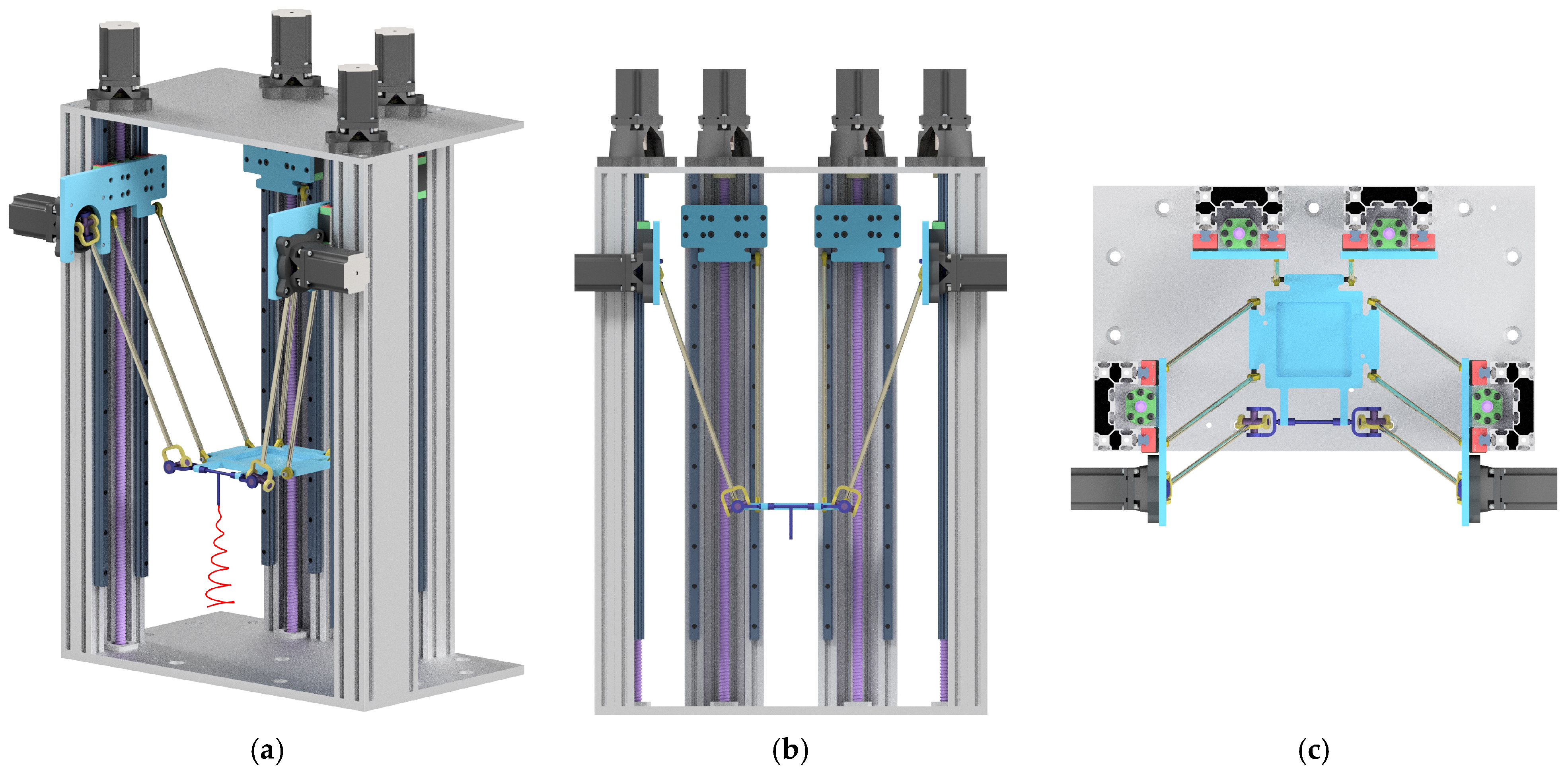
Figure 9 illustrates a computer model of the robot designed in SolidWorks software [29]. The motion range of the robot end-effector along the $Ox$, $Oy$, and $Oz$ axes is 0.297 m, 0.324 m, and 0.424 m, respectively. The moving plate can tilt for $\pm {36}^{\circ }$, and the end-effector rotation range relative to this plate is ${345}^{\circ }$. The base plate, top plate, moving plate, and carriages are made of aluminum alloy. Four vertical columns represent an extruded profile, and each column includes two linear rails attached to the carriage. We use a preliminary chosen Nema 23 stepper motor with a ball screw transmission to actuate each carriage. Similar motors, installed on the side carriages, control the end-effector rotation via two rods with universal joints. All rods are made of carbon fiber.

The first step is to simulate the inverse kinematics of the mechanism. We suppose the end-effector moves at a constant speed of 0.046 m/s along the trajectory analyzed in Section 3.2 and illustrated in Figure 9a. This speed value is selected to achieve a simulation time equal to 10 s. The results of the kinematic simulation are the values of the angular displacement, speed, and acceleration of the motors. The simulation, performed in SolidWorks, shows that the angular displacements are very close to the analytical computations: the average deviation is less than 1%. This deviation is due to the slight discrepancies between the analytical trajectory and the one drawn using CAD tools. These discrepancies are caused by import limitations and different approaches for the linear approximation of the trajectory in the SolidWorks and MATLAB software.

Since the angular displacements are identical for analytical and CAD simulations, we use CAD tools instead of the Jacobian analysis to compute angular speeds ${\omega }_1,\cdots ,{\omega }_5$ and accelerations ${\epsilon }_1,\cdots ,{\epsilon }_5$ of the motors, which are shown in Figure 10. Note that the redundant actuation prevents setting two input motions for the drives that control the end-effector rotation relative to the moving plate. To overcome this issue, only drive $M_l$ (Figure 1), installed on the left carriage, is considered actuated in this and subsequent dynamic analyses.

The next step is to simulate inverse dynamics.

Table 2. Inertial parameters of the movable links of the 5-DOF Delta-type parallel robot.

Link/Group of Links	Material	Inertia Moment/Matrix/(kg·mm2)	Mass/kg
Side carriage with motor (Figure 11a)	Aluminum alloy, steel	–	3.325
Back carriage with nut and sliders (Figure 11b)	Aluminum alloy, steel	–	1.243
Moving plate with joints (Figure 11c)	Aluminum alloy, steel	1384.698	0.488
U-shaped link (Figure 11d)	ABS plastic	1.485	0.006
Yoke (Figure 11e)	Steel	$\left[\begin{array}{ccc}6.711& 0& 0\\ 0& 3.633& 0\\ 0& 0& 3.633\end{array}\right]$	0.043
End-effector (Figure 11f)	ABS plastic	$\left[\begin{array}{ccc}2.703& 0& 0\\ 0& 46.717& -0.011\\ 0& -0.011& 48.330\end{array}\right]$	0.012
Screw (Figure 11g)	Steel	61.061	1.340
U-rod (Figure 11h)	Carbon fiber, ABS plastic	$\left[\begin{array}{ccc}396.966& 0& 0\\ 0& 396.966& 0\\ 0& 0& 2.449\end{array}\right]$	0.021
S-rod (Figure 11i)	Carbon fiber, steel	$\left[\begin{array}{ccc}1049.613& 0& 0\\ 0& 1049.978& 0\\ 0& 0& 0.698\end{array}\right]$	0.041

shows the inertial parameters of the robot movable links, which are used in dynamic computations. The inertia parameters are defined with respect to the axes and reference frames depicted in Figure 11, where point s indicates the center of mass of each link. The links shown in Figure 11a,b perform the translational motion, and Table 2 ignores their moments of inertia. The links shown in Figure 11c,d,g rotate about the $sy$, $sx$, and $sz$ axes, respectively, and Table 2 specifies the inertia moments about these axes. The remaining links shown in Figure 11e,f,h,i perform spatial rotations, and Table 2 specifies the inertia matrices about the depicted reference frames.

After solving the inverse kinematic problem using the SolidWorks software, we import the obtained results to Autodesk Inventor, where they are used as the input motion for solving the inverse dynamic problem. As we mentioned before, only the left auxiliary motor ($M_l$) is active because of the CAD limitations. We assume that it fully supports any load applied to the end-effector, while the second drive ($M_r$) remains passive. As a result, the computed torque will be higher compared with the redundantly actuated case. Because the considered end-effector rotation is decoupled from its other motions, we expect the motor torque will be twice lower in that case.

Figure 12 presents the results of the inverse dynamic simulation. The torque oscillations in this figure match the end-effector motion along the spiral-like trajectory. Torques ${\tau }_1$ and ${\tau }_4$ in the motors translating the side carriages are higher than torques ${\tau }_2$ and ${\tau }_3$ in the motors translating the back carriages. This increase is because the side carriages are equipped with the motors (Figure 11a), and they have higher mass according to Table 2. The minimum value of each of these torques agrees with the force value required to support the carriage weight (we consider the screws with a pitch of 5 mm). Torque ${\tau }_l$ of motor $M_l$, which rotates the end-effector relative to the moving plate, is greater than torques ${\tau }_1,\cdots ,{\tau }_4$, because this motor operates without a ball screw transmission or any other reducer. In practice, we expect to obtain the lower values of torque ${\tau }_l$ because of the redundant actuation, as discussed in the preceding paragraph. However, even with these high torque values, the preliminary chosen stepper motors (Nema 23) are suitable for the considered robot.

6. Discussion

Most of the current research has considered the kinematic analysis of a novel 5-DOF Delta-type robot, and here, we discuss some issues of this analysis. The algorithm for solving the inverse kinematic problem is straightforward: we should only check that the considered configuration of the robot belongs to its workspace to avoid complex solutions of Equation (4). The forward kinematics is more challenging to solve. The method we used to address this problem resembles familiar elimination approaches [30,31,32], applied to Delta-type robots as well [12,33,34]. Unlike most of these works, we do not need to compute a resultant of polynomial equations to obtain the final Equation (19), which simplifies the elimination procedure. At the same time, the forward kinematics has several caveats.

When we derived Equation (18), we assumed $F_0\ne 0$. In this case, we compute different values of angle ${\phi }_p$ following the developed algorithm. Parameter $F_0$ depends on this angle, and we cannot certify that all the obtained solutions do not make it equal to zero. If $F_0=0$ for some angle ${\phi }_p$, we cannot use Equation (14) to find $x_{C4}$, $y_{C4}$, and $z_{C4}$, because matrix $\mathbf{A}$ degenerates. To solve the forward kinematics, we should consider two independent linear equations of Equation (14) and quadratic Equation (13): we can get one quadratic equation with respect to a single variable by eliminating two others using the linear equations. In this case, we get two different moving plate configurations for a single value of angle ${\phi }_p$. For example, with the “symmetrical” geometry considered in Section 3.2 and with $h_1=\dots =h_4$, we have solution ${\phi }_p=0$ (the moving plate is horizontal), which makes $F_0=0$. Using the procedure above, we obtain two configurations of the moving plate for this angle: when it is above or below the carriages. If the rank of matrix $\mathbf{A}$ drops by two, there are no three independent equations to find $x_{C4}$, $y_{C4}$, and $z_{C4}$. As a result, the forward kinematic problem has an infinite number of solutions, and the robot is probably in a singular configuration—this analysis is beyond the current article. However, we note that the robot singularities only depend on the configuration of its 4-DOF part. This is because the fifth DOF (the end-effector rotation) is decoupled from other motions, and configurations of the two auxiliary branches do not affect the 4-DOF part of the robot and its singularities, which were studied in [26].

Finally, we also cannot guarantee that the eighth-degree polynomial Equation (19) has eight real solutions corresponding to eight different assembly modes of the robot. Furthermore, even if we obtain eight real solutions of this equation, we cannot assert that $F_0\ne 0$ for all the solutions. These problems are beyond the scope of this article, and we will consider them in the future.

7. Conclusions

This article has studied a novel 5-DOF redundantly actuated Delta-type parallel robot. The robot end-effector has three translational and two rotational DOFs, and one rotation is controlled by two drives. This redundant actuation makes the robot design symmetrical and helps distribute the load between the drives more evenly.

First, we have developed the algorithm to solve the inverse kinematic problem. The algorithm provides us with a closed-form solution to this problem, which was illustrated with the trajectory simulation example. Next, we have considered the forward kinematics of the robot. We have proposed a procedure that reduces this problem to solving the eighth-degree polynomial equation. Its roots correspond to various assembly modes of the robot. The numerical example has presented a case with four real solutions and four assembly modes. Determining the maximum possible number of these modes is an open issue that we will solve in the future.

Finally, we have used SolidWorks and Autodesk Inventor to design a computer model of the robot and perform inverse kinematic and dynamic simulations. The CAD tools simplify dynamic computations and allow us to consider complex shapes and inertial parameters of the robot links as accurately as possible. As an example, we have solved the inverse dynamic problem and computed the motor torques required to follow the spatial trajectory analyzed in the inverse kinematics.

The proposed kinematic algorithms represent the basis for workspace analysis and singularity determination of the robot, which will be performed in future studies. These techniques can be adapted to other parallel robots as well. We will also use the results of CAD simulations to create a physical prototype of the discussed robot.