Abstract
This paper introduces a novel fuzzy logic switched model predictive control (MPC) algorithm for articulated steering vehicles, addressing significant path tracking challenges due to varying road conditions and vehicle speeds. Traditional single-model and parameter-based controllers struggle with tracking errors and computational inefficiencies under diverse operational conditions. Therefore, a kinematics-based MPC algorithm is first developed, showing strong real-time performance but encountering accuracy issues on low-adhesion surfaces and at high speeds. Then, a 4-DOF dynamics-based MPC algorithm is designed to enhance tracking accuracy and control stability. The proposed solution is a switched MPC strategy, integrating a fuzzy control system that dynamically switches between kinematics-based and dynamics-based MPC algorithms based on error, solution time, and heading angle indicators. Subsequently, simulation tests are conducted using SIMULINK and ADAMS to verify the performance of the proposed algorithm. The results confirm that this fuzzy-based MPC algorithm can effectively mitigate the drawbacks of single-model approaches, ensuring precise, stable, and efficient path tracking across diverse adhesion road conditions.
1. Introduction
Articulated steering vehicles (ASVs), characterized by separate front and rear bodies with steering achieved through relative rotation, are noted for their exceptional maneuverability, adaptability, and high load-bearing capacity. Examples include articulated trucks and loaders, which are primarily deployed in enclosed environments like mines and farmlands rather than on urban roads. Implementing autonomous driving technology in these engineering vehicles offers significant benefits, including enhanced safety, increased productivity, and reduced operational costs.
To implement path tracking for ASVs, the first step is to construct a vehicle model that accurately describes its motion characteristics [1]. Currently, classic kinematic models of ASVs are widely used to depict changes in position, heading, and articulation angles based on inputs such as speed and articulation angular velocity [2]. For example, Nayl et al. proposed a kinematic model incorporating vehicle sideslip to enhance tracking accuracy [3]. However, kinematic models do not account for the internal forces within the vehicle, resulting in inadequate accuracy under conditions of high speed and low traction. Although some existing research has established dynamic models for ASVs primarily to analyze the vehicle’s stability and steering characteristics [4,5,6], few have used these models for path tracking control [7,8]. This is because dynamic models involve numerous variables with complex interrelationships and parameters that are difficult to estimate accurately, leading to significantly higher computational difficulty and time requirements compared to kinematic models.
Furthermore, researchers have developed various control algorithms for path tracking based on these vehicle models, such as sliding mode controllers [9], LQR controllers [10], feedback linearization controllers [11,12], and model predictive control (MPC) [2,7,13,14,15]. MPC has garnered significant attention in recent years due to its effectiveness in handling multi-input, multi-constraint vehicle control problems [16]. However, most of these control algorithms for ASVs [2,7,13,15] are based on constant controller parameters, which may lead to suboptimal performance under varying road conditions and vehicle speeds, particularly in scenarios involving low adhesion, high speed, and sharp turns.
Some studies have attempted to address the effects of road adhesion and speed on vehicle tracking for other vehicle types. For instance, Li et al. developed a H∞ state feedback controller tailored for a LPV system, accounting for uncertainties in vehicle longitudinal speed and road adhesion coefficients [17]. Hang et al. introduced an LQR control approach based on a LPV system, treating vehicle speed and road adhesion coefficient as variable parameters [18]. Tang et al. proposed an MPC controller that adapts to speed-variable dynamics [19]. Despite these advancements, accurately estimating road adhesion coefficients remains challenging, and incorrect estimations can lead to increased tracking errors. To mitigate this issue, Chen et al. integrated vehicle sideslip angle into a handling stability control framework for sideslip compensation [20].
Some studies integrate fuzzy logic systems with tracking controllers to enhance the controller’s adaptability to varying parameters. For instance, He et al. proposed a fuzzy-based speed parameter switching strategy to ensure better adaptability [21]. Rokonuzz et al. developed a fuzzy-based switched MPC algorithm that switches between vehicle kinematic and dynamic models [22], which can improve computational efficiency and tracking accuracy. Additionally, Awad et al. developed a multi-input multi-output linear MPC algorithm with fuzzy logic switching based on the vehicle’s heading angle [23]. For ASVs, Alshaer proposed a fuzzy control algorithm that uses tracking error as input and articulation angle and speed as outputs, enabling the vehicle to quickly converge to the desired path [24]. Although existing research [22] has implemented MPC with fuzzy switching strategy between kinematics and dynamics, it focuses on front-wheel-steering vehicles operating on structured road, and therefore cannot be applied to articulated steering vehicles.
In summary, a single set of parameters and models of ASVs cannot yield optimal results under complex road conditions, potentially compromising control accuracy and computational efficiency during path tracking. To address these challenges, this paper proposes a switched MPC algorithm based on multiple vehicle models and parameters. The main contributions of this paper are as follows:
- (1)
- A new kinematics-based nonlinear MPC (KNMPC) controller—to ensure both tracking accuracy and computational efficiency by incorporating the vehicle sideslip angle into the kinematic model.
- (2)
- A new 4-DOF dynamics-based linearized MPC (DLMPC)—to enhance tracking accuracy under low adhesion road conditions and high speeds by considering tire-ground interaction.
- (3)
- A novel fuzzy-based switched MPC approach—to ensure accurate and efficient path tracking under diverse road conditions simultaneously. This approach can facilitate the transition between KNMPC and DLMPC.
- (4)
- Effective simulations by SIMULINK and ADAMS—to evaluate and verify the performance of KNMPC, DLMPC, and the switched MPC.
The remainder of the paper is organized as follows. Section 2 provides a brief description of the kinematic and dynamic models employed. The design and comparison of KNMPC and DLMPC are detailed in Section 3. Section 4 presents the design of the fuzzy-based switched MPC strategy. Subsequently, experimental results and analysis for the switched MPC controller are presented in Section 5. Finally, a brief conclusion and future work are provided in Section 6.
2. Vehicle Modeling
This section presents a kinematic model and a 4-DOF dynamic model for an ASV. The kinematic model accounts for sideslip angle. The 4-DOF dynamic model includes the longitudinal, lateral, and yaw motions of the front vehicle body, as well as the yaw motion of the rear vehicle body. Figure 1 shows the models, and Table 1 lists their symbols.
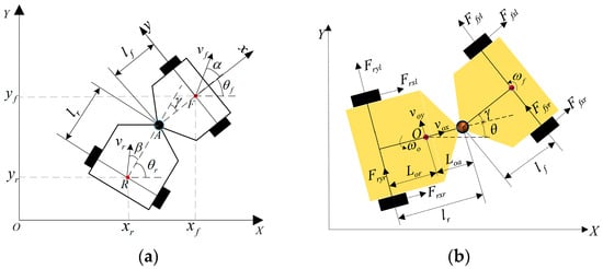
Figure 1.
(a) Geometry of kinematic model and (b) geometry of dynamic model.

Table 1.
List of nomenclature.
2.1. Kinematic Model
To improve the accuracy of the kinematic model, we deploy the slip angle based on the model in [3]. The geometry of kinematic model is shown in Figure 1a. We assume that the vehicle moves on a horizontal plane and its vertical motion is neglected. Also, assuming the vehicle is in a steady-state steering condition, the variation in joint angular velocity is small.
Taking point F as the tracking reference point and considering the sideslip angle, the changes in the lateral and longitudinal directions in the global coordinate system can be expressed as:
During steady-state motion, the relative velocity between the front and rear bodies at the articulation point is zero. Defining the counterclockwise direction as positive for rotation, the motion constraint relationship at the articulation point between the front and rear bodies can be expressed as:
where is the rotation matrix for the point transformation between the front body coordinate system and the rear vehicle body coordinate system, with the articulation angle being the rotation angle.
According to the geometry of kinematic model in Figure 1a, the relationship between the heading angle of the rear body, the articulation angle, and the heading angle of the front body is:
By combining (1)–(3), we can obtain the kinematic model at reference point F as:
where .
The sideslip angle describes the angle difference between the actual direction of vehicle travel and the orientation of the vehicle body. It can be expressed as
2.2. Dynamic Model
A diagram of the dynamic model is shown in Figure 1b, constructing a coordinate system fixed to the vehicle body with the centroid of the entire vehicle O as the origin. This model is primarily used to describe the lateral characteristics considering the effects of tire–ground interaction. For the sake of calculation convenience, some simplifications are made as follows:
- (1)
- We assume the vehicle travels on a flat road surface, neglecting vertical motion.
- (2)
- We assume the connection between the front and rear bodies is rigid, neglecting motion coupling between steering systems and swing axles.
- (3)
- We neglect the lateral load transfer of tires during steering.
- (4)
- We neglect the coupling relationship between longitudinal and lateral forces of the tires and consider the vehicle’s lateral and longitudinal motions separately during modeling.
Based on Newton’s second law and Euler’s formula, the force equilibrium equations in the X and Y axis of the vehicle, as well as the moment equilibrium equation about the Z axis, can be derived as:
According to assumption (3), the forces acting on the two-side tires are approximated as equal, and the tire forces are linearly described [6]. Therefore, the lateral and longitudinal forces of the front and rear tires can be represented as:
The lateral and longitudinal velocities at the center point of the front wheel axle are represented as:
By combining (6)–(8), the dynamic model can be represented as:
where , and .
3. MPC Controller Design and Tracking Error Comparison
Model predictive control (MPC) is a control strategy that continuously optimizes control actions to achieve the best possible performance based on a defined cost function while ensuring that constraints, such as actuator saturation, safety, and stability, are satisfied. The future states of the vehicle are forecasted by a predictive model and used for optimizing the control action, consequently enhancing control accuracy. In this section, we use the kinematic and dynamic models constructed in Section 2 as the predictive models and design model predictive controllers, accordingly, serving as the base controllers for the switching control. We also compare their performance under different adhesion coefficients and speeds.
3.1. Kinematics-Based Nonlinear MPC
Firstly, we design a kinematics-based nonlinear MPC considering vehicle sideslip angle. The kinematic model in Equation (4) is simplified as:
where are the state variables and are the control input variables.
The discrete-time state-space equations, based on the forward Euler method, are established as follows:
where T is the step size.
Due to the fewer number of state variables and their simpler relationships, the kinematic model is easy to solve. Therefore, we retain the nonlinearity of the kinematic model. By directly expanding Equation (11), the vehicle states within the control horizon and the prediction horizon can be expressed as:
To ensure the vehicle tracks accurately and smoothly along the desired path, a cost function [22] is designed in Equation (13).
where represents the displacement error, represents the heading angle error, and represents the control input increment for a single control step. and are the weight matrices corresponding to the state errors, is the weight matrix for the control input increments, and is a quadratic relaxation factor used to improve the efficiency of the solution.
To ensure the solved values align with the vehicle performance, the constraints are set as follows:
3.2. Dynamics-Based Linear MPC
Second, we design a dynamics-based linear MPC to improve accurate path tracking at low adhesion and higher speeds. Similarly, according to Equation (10), the dynamic model can be simplified as:
where are the state variables and is the control input variable.
Due to the numerous state variables in the dynamic model, solving the nonlinear model is inefficient. Therefore, the model is linearized by performing a Taylor expansion around point and retaining the first-order terms, resulting in:
where the system matrix and input matrix are given as follows, respectively:
Further discretizing Equation (16), we obtain:
where , , and is the identity matrix.
According to Equation (12), we further expand Equation (17) within the control horizon Nc and the prediction horizon Np and then solve for the control variable based on Equation (13). In addition to considering the vehicle motion constraints and control increment constraints associated with the kinematics-based MPC discussed above, dynamic solutions can also incorporate constraints such as lateral acceleration to ensure vehicle stability during motion. The optimization problem of DLMPC can be represented in the following form:
where is the maximum value of control variables, is the maximum value of control increment, and is the maximum value of state variables. is a dimensional unit column vector.
3.3. Tracking Error Comparison
To verify the tracking performance of the controllers on regular and extreme road conditions, we conducted the tests on different adhesion road surfaces at different speeds. The common U-shaped paths found in agriculture and mining were used as the desired paths to verify the controller’s tracking capabilities along both straight and turning trajectories. The desired path, depicted in Figure 2, comprises a straight segment of length L = 20 m followed by a curved arc with a radius of R = 2 m. According to the driving environment [25], experiments were conducted separately on high-adhesion surfaces with an adhesion coefficient of 0.8 and low-adhesion surfaces with an adhesion coefficient of 0.4.
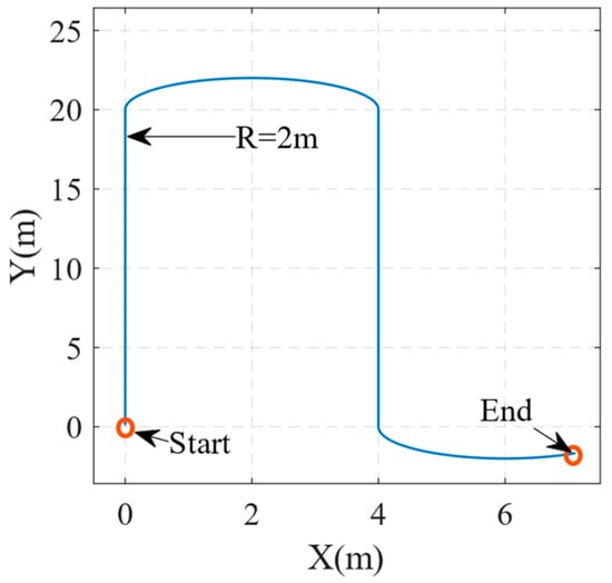
Figure 2.
The desired path in the tests.
Figure 3 shows the result on the road with the adhesion coefficient of 0.8. The vehicle speeds were 1 m/s and 2 m/s, respectively. Figure 3c illustrates the result in KNMPC. When the speed was 1 m/s, the displacement error remained within a range of 0.06 m both straight motion and turning. However, when the speed increased to 2 m/s, the maximum displacement error in the turning trajectory increased to approximately 0.15 m. From Figure 3d, it can be observed that on high-adhesion road surfaces, the displacement error of DLMPC is similar in magnitude to that of KNMPC. However, the average solving time of DLMPC is higher than that of KNMPC.
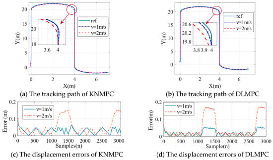

Figure 3.
Tracking performance of the controllers on the road with the adhesion coefficient of 0.8.
Secondly, evaluation was conducted on a road with an adhesion coefficient of 0.4. The vehicle speeds were 1 m/s and 2 m/s, respectively. The results are depicted in Figure 4. Figure 4c shows a significant deviation made by KNMPC when tracking the turning path at 1 m/s and 2 m/s, i.e., maximum displacement errors of 0.56 m and 0.63 m, respectively. Figure 4d shows the maximum displacement errors of DLMPC, i.e., 0.07 m and 0.19 m, respectively. By incorporating the relationship between tire forces and vehicle yaw into the dynamic model, DLMPC can consider the impact of slip-on vehicle position when calculating control inputs. As a result, the controller demonstrates improved performance on low-adhesion roads with significant slip. As shown in Figure 4e,f, DLMPC required more computation time than KNMPC.
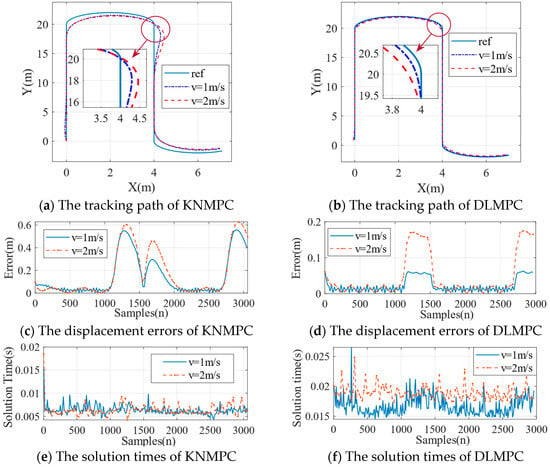
Figure 4.
Tracking performance of the controllers on the road with the adhesion coefficient of 0.4.
4. Switched MPC Strategy Design
According to the results in Section 3.3, KNMPC has demonstrated higher tracking accuracy under high adhesion and low-speed conditions, whereas DLMPC maintains good tracking accuracy under low adhesion and high-speed conditions. In terms of computational efficiency, KNMPC is more efficient than DLMPC and requires less hardware computational power. Given the diverse road adhesion coefficients encountered during vehicle operation, controllers that rely on a single parameter or model struggle to maintain both control accuracy and computational efficiency simultaneously.
To address this challenge, we propose a switched MPC strategy with multiple models and parameters, which is illustrated in Figure 5. This approach includes four sub-controllers in which KNMPC1 and KNMPC2 are nonlinear MPCs based on the kinematic model, DLMPC1 and DLMPC2 are linear MPCs based on the dynamic model. Each model-based controller employs two distinct sets of Np and Nc parameters to enhance adaptability to roads with varying curvatures. These controllers compute control outputs (articulation angle and speed) based on the current and desired vehicle states. The model prediction errors, solution times across different models, and heading angle increments are introduced as switching costs. A fuzzy logic switch then selects the appropriate sub-controller based on the switching strategy for the path tracking control of ASV.
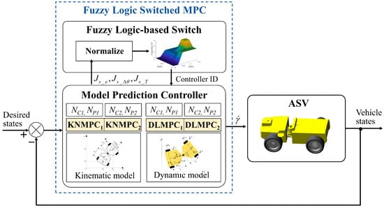
Figure 5.
Schematics of the proposed switched MPC.
4.1. Switching Cost
To achieve more rational and efficient application of sub-controllers under different working conditions, a fuzzy logic-based switching strategy was designed. The switching costs between the kinematic and dynamic models were taken as input to provide a suitable model selection as output. This strategy switches between different parameters and controllers according to the cost function:
where is the switching strategy, is cost function, and is the controller ID.
The switching cost indicators include the predictive position errors , the increment of desired heading angle , and the solution times of different models . The model predictive error directly reflects the predictive accuracy of the model at the current time. To improve efficiency, we only selected the most relevant state variables to path tracking, the X and Y coordinates and the heading angle, as the variables for evaluating predictive error [26]. The states under the current inputs are calculated using the prediction model in Equation (12), and these predicted states are then compared with the desired states at future Np steps. The predictive error is obtained by averaging the error over Np steps. The calculation formula is:
where are the current position and the desired position at future time steps, and are the positions given by the predictive model. is the current heading angle and the desired states at future time steps, and is the heading angle given by the predictive model.
Tracking error usually increases during steering. The rate of change of the heading angle reflects the trend of path curvature variation, making it a suitable indicator for switching strategy. This value is obtained by calculating the deviation between the current heading angle and the desired heading angle at time t.
The solution time is also an important indicator to consider during the control process, as it reflects the computational efficiency of the controller. This value is obtained by collecting the solution time of the controller, and the formula is expressed as:
where is the solution time for the controller at time , and is the number of time steps in which the controller is active. To prevent the solution time from being zero, each controller is assigned an initial value obtained from previous experiments.
By introducing appropriate weights, three indicators are added together to obtain the switching cost function. These weights provide the flexibility for designing the appropriate switching cost.
where represent the weights corresponding to each indicator. These weights allow the switching cost function to be adjusted flexibly according to requirements. A larger prioritizes tracking accuracy; a larger prioritizes heading stability; and a larger prioritizes the speed of computation.
Due to the significant differences in dimensions among the indicators, it is necessary to appropriately normalize the values of each indicator before calculating the switching cost. The normalization formula is as follows:
where is a vector composed of indicators at different steps, and and are the maximum and minimum values in the vector, respectively.
4.2. Fuzzy Logic-Based Switching
To create a knowledge database, the vehicle was driven on roads with different adhesion coefficients: 0.4, 0.6 and 0.8. For each road condition, different maneuvers such as straight driving and turning were performed. The vehicle was driven at speeds of 1 m/s and 2 m/s. To achieve higher tracking accuracy while ensuring computational efficiency, we conducted multiple trial-and-error comparisons with different weight configurations and determined the optimal weights. The optimal weights were determined to be 0.8, 0.6 and 0.5, respectively.
Figure 6 shows the range of cost values for each model. We fuzzified the switching cost into three fuzzy subsets , where S means ‘Small’, M means ‘Medium’ and L means ‘Large’. The switching cost domain for KNMPC is [0, 1.5], and that for DLMPC is [0, 1].
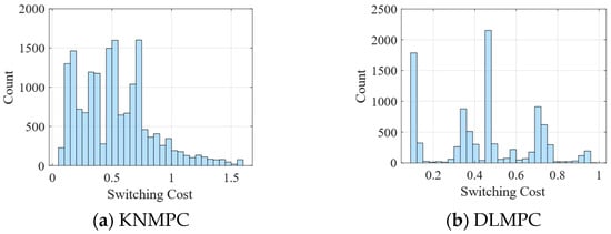
Figure 6.
Switching cost for different models.
Based on the knowledge base, the appropriate membership function for each input variable is designed. Considering the dynamic variation characteristics of the input switching cost, we choose the trapezoidal membership function [27] for the fuzzification of the input variables. This membership function is expressed as:
where represents the membership degree when the input variable value is . and define the width of the trapezoid. and determine the slopes of the trapezoid. Figure 7 shows the input fuzzy sets with their degree of membership.

Figure 7.
Membership functions for each input variable.
The input fuzzy sets are linked through a set of fuzzy rules to provide an output. The output of the fuzzy controller is , corresponding to the controller IDs . Considering the advantages of KNMPC, such as fewer parameters and simpler calculations, the rules are primarily designed to preferentially select KNMPC whenever possible. DLMPC is chosen only when the kinematic cost value is greater than the dynamic cost value. Additionally, larger values of control horizon and predictive horizon enable the controller to achieve smaller tracking errors during steering [28]. Therefore, the controller with larger values of control horizon and predictive horizon is chosen when the cost value is large. The fuzzy rules are established as shown in Table 2.

Table 2.
The fuzzy rules to select controllers.
Figure 8 shows the output of the fuzzy controller for various combinations of switching cost inputs. We employ a Sugeno fuzzy inference system utilizing AND rules. The final output of the controller is represented as:
where is the number of activated rules, is the number of input variables, is the output value of the jth rule.
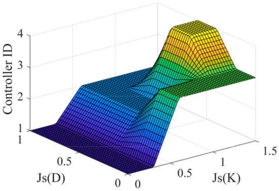
Figure 8.
The output of the fuzzy controller.
The overall flow chart of fuzzy switched MPC algorithm is summarized in Figure 9.
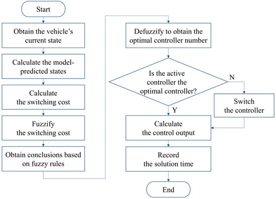
Figure 9.
The overall flow chart of fuzzy logic switched MPC.
5. Results and Discussion
The tests in the paper are conducted utilizing MATLAB/Simulink and ADAMS. They are run within an Intel Core i7-13700 CPU with 32 GB RAM. The ADAMS model is based on a 1:4 articulated engineering vehicle prototype, as shown in Figure 10. Detailed parameters of the ADAMS model are listed in [29]. In the ADAMS environment, the tire model utilizes the magic formula tire model, with parameters such as tire radius, lateral stiffness, longitudinal stiffness defined. The road surface utilizes a customizable surface with adjustable coefficients of friction. By modifying the adhesion coefficient for corresponding road segments, simulations under various adhesion coefficients can be conducted. The models and controller’s parameters are shown in Table 3 and Table 4, respectively.

Figure 10.
The ADAMS model.

Table 3.
The model parameters.

Table 4.
The controller parameters.
To validate the performance of the switched controller, a variable adhesion road surface condition was constructed in ADAMS in conjunction with a U-shaped desired path. The adhesion coefficient parameters were set as shown in Figure 11. As described in Section 4, the system is composed of four basic controllers, defined as Mi1 to Mi4. Mi1 is a KNMPC with parameters Np1 and Nc1, Mi2 is a KNMPC with parameters Np2 and Nc2, Mi3 is a DLMPC with parameters Np1 and Nc1, and Mi4 is a DLMPC with parameters Np2 and Nc2. The displacement error and the solution time per for each control input are used to evaluate the tracking accuracy and algorithm efficiency.
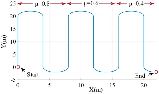
Figure 11.
Adhesion coefficient parameters of the desired path.
The choice of models in the different sections of the path during the tracking task is shown in Figure 12a. The blue and green points represent KNMPC with different control parameters, while the yellow and red points represent DLMPC with different control parameters. First, the vehicle speed is set to 1 m/s. Based on the distribution of the points, when the adhesion coefficient is , the KNMPC is primarily chosen. As the adhesion decreases to and , the DLMPC starts to be adopted during turning. Additionally, on the straight path, control parameters with shorter prediction and control horizons are selected, whereas when tracking the turning path, control parameters with larger prediction and control horizons are chosen.
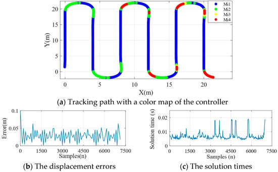
Figure 12.
Tracking performance at 1 m/s.
When the vehicle speed is 2 m/s, the results are shown in Figure 13. Compared to the speed of 1 m/s, the number of points using DLMPC during turns significantly increases. Additionally, as the speed increases, the proportion of controllers Mi2 and Mi4 with larger Np2 and Nc2 increases. As stated in reference [27], the parameters Np and Nc in the MPC should grow as v increases. Compared to using a single KNMPC, the switched controller can maintain higher accuracy. And it has a lower average solution time compared to using a single DLMPC.
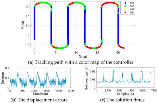
Figure 13.
Tracking performance at 2 m/s.
Table 5 summarizes the results of single controllers and the switched controller on low adhesion road. The switched controller effectively improves the accuracy and stability of KNMPC on low-adhesion road, as well as the real-time performance of DLMPC. Under high-speed conditions, the average error of switched MPC is reduced by 62.5% compared to that of KNMPC. The processing time of our switched MPC is 57.9% less than that of DLMPC. Furthermore, as seen from the solution times in Table 5, the introduction of fuzzy switching strategy did not significantly increase the algorithm’s solution time. This indicates that the time complexity of the proposed algorithm is like that of a single KNMPC, and it can meet the real-time requirements in practical applications.

Table 5.
Results of tracking path.
6. Conclusions
This study provides an efficient switching control framework designed for driving conditions with varying adhesion coefficients. Firstly, a kinematic model incorporating slip angle and a 4-DOF dynamic model were established. Subsequently, a fuzzy-based switched MPC strategy was implemented to facilitate controller switching. Experimental results have demonstrated the superior overall performance of the proposed switched MPC framework. The proposed fuzzy logic switched model predictive control (MPC) model can dynamically switch controllers based on a cost function that considers predictive error, solution time, and heading angle increments.
In future works, we will consider additional switching cost function indicators, such as lateral stability indicators and actuator response time. Additionally, the selection of parameters in a fuzzy logic control system has a significant impact on the performance of the system. Therefore, adaptive parameter adjustment by a reinforcement learning algorithm will be introduced to enhance the controller’s adaptability to different tracking demands.
Author Contributions
Methodology, X.C.; software, J.C.; formal analysis, Y.G.; investigation, G.S.; writing—original draft preparation, Q.Z. and X.C.; writing—review and editing, H.H.; resources, Q.Z. and H.H. All authors have read and agreed to the published version of the manuscript.
Funding
This research was funded by China Tobacco’s “Selecting Best Projects by Opening Competition Mechanism” Program, grant number 110202301013-2, The Key Technology Innovation and Industrialization Program of Fujian Province, grant number 2023XQ021, University-Industry Collaborative Program of Fujian Province, grant number 2021H6019, the National Natural Science Foundation of China, grant number 52075461.
Data Availability Statement
The raw data supporting the conclusions of this article will be made available by the authors on request.
Conflicts of Interest
The authors declare no conflicts of interest.
References
- Qu, J.; Zhang, Z.; Qin, Z.; Guo, K.; Li, D. Applications of Autonomous Navigation Technologies for Unmanned Agricultural Tractors: A Review. Machines 2024, 12, 218. [Google Scholar] [CrossRef]
- Song, R.; Ye, Z.; Wang, L.; He, T.; Zhang, L. Autonomous Wheel Loader Trajectory Tracking Control Using LPV-MPC. In Proceedings of the 2022 American Control Conference, Atlanta, GA, USA, 8–10 June 2022. [Google Scholar]
- Nayl, T.; Nikolakopoulos, G.; Gustafsson, T. A full error dynamic switching modeling and control scheme for an articulated vehicle. Int. J. Control Autom. Syst. 2015, 13, 1221–1232. [Google Scholar] [CrossRef]
- Pazooki, A.; Rakheja, S.; Cao, D. Kineto-dynamic directional response analysis of an articulated frame steer vehicle. Int. J. Veh. Des. 2014, 65, 1–30. [Google Scholar] [CrossRef]
- Li, X.; Wang, G.; Yao, Z.; Qu, J. Dynamic model, and validation of an articulated steering wheel loader on slopes and over obstacles. Veh. Syst. Dyn. 2013, 51, 1305–1323. [Google Scholar] [CrossRef]
- Zhu, Q.; Yang, C.; Hu, H.; Wu, X. Building a novel dynamics rollover model for critical instability state analysis of articulated multibody vehicles. Int. J. Heavy Veh. Syst. 2021, 28, 329–352. [Google Scholar] [CrossRef]
- Shi, J.; Sun, D.; Qin, D.; Hu, M.; Kan, Y.; Ma, K.; Chen, R. Planning the trajectory of an autonomous wheel loader and tracking its trajectory via adaptive model predictive control. Robot. Auton. Syst. 2020, 131, 103570. [Google Scholar] [CrossRef]
- Shahirpour, A.; Abel, D. Simulation, and successive sideslip-compensating model predictive control for articulated dump trucks. In Proceedings of the IEEE 25th International Conference on Intelligent Transportation Systems (ITSC), Macau, China, 8–12 October 2022. [Google Scholar]
- Nayl, T.; Nikolakopoulos, G.; Gustafsson, T.; Kominiak, D.; Nyberg, R. Design, and experimental evaluation of a novel sliding mode controller for an articulated vehicle. Robot. Auton. Syst. 2018, 103, 213–221. [Google Scholar] [CrossRef]
- Yu, H.; Zhao, C.; Li, S.; Wang, Z.; Zhang, Y. Pre-work for the birth of driver-less scraper (LHD) in the underground mine: The path tracking control based on an LQR controller and algorithms comparison. Sensors 2021, 21, 7839. [Google Scholar] [CrossRef]
- Dekker, L.G.; Marshall, J.A.; Larsson, J. Experiments in feedback linearized iterative learning-based path following for center-articulated industrial vehicles. J. Field Robot. 2019, 36, 955–972. [Google Scholar] [CrossRef]
- Zhao, X.; Yang, J.; Zhang, W.; Zeng, J. Feedback linearization control for path tracking of articulated dump truck. Telkomnika 2015, 13, 922–929. [Google Scholar] [CrossRef][Green Version]
- Bai, G.; Liu, L.; Meng, Y.; Luo, W.; Gu, Q.; Ma, B. Path tracking of mining vehicles based on nonlinear model predictive control. Appl. Sci. 2019, 9, 1372. [Google Scholar] [CrossRef]
- Nayl, T.; Nikolakopoulos, G.; Gustafsson, T. Effect of kinematic parameters on MPC based on-line motion planning for an articulated vehicle. Robot. Auton. Syst. 2015, 70, 16–24. [Google Scholar] [CrossRef]
- Zhou, B.; Su, X.; Yu, H.; Guo, W.; Zhang, Q. Research on Path Tracking of Articulated Steering Tractor Based on Modified Model Predictive Control. Agriculture 2023, 13, 871. [Google Scholar] [CrossRef]
- Stano, P.; Montanaro, U.; Tavernini, D.; Tufo, M.; Fiengo, G.; Novella, L.; Sorniotti, A. Model predictive path tracking control for automated road vehicles: A review. Annu. Rev. Control 2023, 55, 194–236. [Google Scholar] [CrossRef]
- Li, P.; Lam, J.; Lu, R. Robust switched velocity-dependent path-following control for autonomous ground vehicles. IEEE Trans. Intell. Transp. 2023, 24, 4815–4826. [Google Scholar] [CrossRef]
- Hang, P.; Chen, X. Path tracking control of 4-wheel-steering autonomous ground vehicles based on linear parameter-varying system with experimental verification. Proc. Inst. Mech. Eng. Part I J. Syst. Control. Eng. 2019, 235, 411–423. [Google Scholar] [CrossRef]
- Tang, Z.; Xu, X.; Wang, F.; Jiang, X.; Jiang, H. Coordinated control for path following of two-wheel independently actuated autonomous ground vehicle. IET Intell. Transp. Syst. 2019, 13, 628–635. [Google Scholar] [CrossRef]
- Chen, Y.; Chen, S.; Ren, H.; Gao, Z.; Liu, Z. Path tracking and handling stability control strategy with collision avoidance for autonomous vehicles under extreme conditions. IEEE Trans. Veh. Technol. 2020, 69, 14602–14617. [Google Scholar] [CrossRef]
- He, Y.; Wu, J.; Xu, F.; Liu, X.; Wang, S.; Cui, G. Path Tracking Control Based on TS Fuzzy Model for Autonomous Vehicles with Yaw Angle and Heading Angle. Machines 2024, 12, 375. [Google Scholar] [CrossRef]
- Rokonuzz, M.; Mohajer, N.; Nahavandi, S. Effective adoption of vehicle models for autonomous vehicle path tracking: A switched MPC approach. Veh. Syst. Dyn. 2022, 61, 1236–1259. [Google Scholar] [CrossRef]
- Awad, N.; Lasheen, A.; Elnaggar, M.; Kamel, A. Model predictive control with fuzzy logic switching for path tracking of autonomous vehicles. ISA Trans. 2022, 129, 193–205. [Google Scholar] [CrossRef] [PubMed]
- Alshaer, B.J.; Darabseh, T.T.; Momani, A.Q. Modelling and control of an autonomous articulated mining vehicle navigating a predefined path. Int. J. Heavy Veh. Syst. 2014, 21, 152–168. [Google Scholar] [CrossRef]
- Zhang, Z.; Xie, L.; Lu, S.; Wu, X.; Su, H. Vehicle yaw stability control with a two-layered learning MPC. Veh. Syst. Dyn. 2023, 61, 423–444. [Google Scholar] [CrossRef]
- Wang, W.; Wang, X. Research on robot indoor localization method based on wireless sensor network. In Proceedings of the 2015 International Conference on Advances in Mechanical Engineering and Industrial Informatics, Zhengzhou, China, 11–12 April 2015. [Google Scholar]
- Lee, H.J.; Park, J.B.; Chen, G. Robust fuzzy control of nonlinear systems with parametric uncertainties. IEEE Trans. Fuzzy Syst. 2001, 9, 369–379. [Google Scholar]
- Wang, M.; Niu, C.; Wang, Z.; Jiang, Y.; Jian, J.; Tang, X. Model and Parameter Adaptive MPC Path Tracking Control Study of Rear-Wheel-Steering Agricultural Machinery. Agriculture 2024, 14, 823. [Google Scholar] [CrossRef]
- Yang, C.; Zhu, Q.; Liu, Q.; Chen, X. An unscented Kalman filter based velocity estimation method for articulated steering vehicles using a novel dynamic model. Proc. Inst. Mech. Eng. Part K J. Multi-Body Dyn. 2023, 237, 389–405. [Google Scholar] [CrossRef]
Disclaimer/Publisher’s Note: The statements, opinions and data contained in all publications are solely those of the individual author(s) and contributor(s) and not of MDPI and/or the editor(s). MDPI and/or the editor(s) disclaim responsibility for any injury to people or property resulting from any ideas, methods, instructions or products referred to in the content. |
© 2024 by the authors. Licensee MDPI, Basel, Switzerland. This article is an open access article distributed under the terms and conditions of the Creative Commons Attribution (CC BY) license (https://creativecommons.org/licenses/by/4.0/).