Kinematic Reliability of Manipulators Based on an Interval Approach ^†

Abstract

Robotic manipulators inevitably experience the impact of uncertainties and errors, such as dimensional tolerances and joint clearances. Therefore, this paper proposes a novel method based on an interval approach to evaluate the kinematic reliability of manipulators. Kinematic reliability quantifies the probability of positioning errors that fall within allowable boundaries. As a result, reliability evaluates the probability that the interval end-effector error produced by dimensional tolerances exceeds an acceptable rate. The proposed reliability index is based on the interval error that conveys an alternative approach to the kinematic reliability methods based on probabilistic frameworks reported in the literature based on probabilistic approaches. The obtained numerical results demonstrate the viability of the proposed methodology by evaluating the reliability of a serial manipulator subjected to joint clearances and a parallel manipulator with dimensional tolerances.

1. Introduction

Errors and uncertainties have an inevitable impact on mechanisms and robotic manipulators. Kinematic reliability ascertains the probability of errors exceeding an allowable limit. Numerous research investigations have concentrated on the reliability analysis of manipulators subjected to errors, and kinematic reliability has been widely used in the analysis of manipulator errors [1]. There are several sources of uncertainties, such as sensor inaccuracies, joint backlash, calibration errors, and unpredictable environmental conditions. The effects of these errors can produce a reduction in positional accuracy, poor trajectory tracking, and failures in precision-dependent applications. Consequently, the enhancement of reliability, accuracy, and overall performance of robotic manipulators demands the analysis of the effects of uncertainties.

A novel hybrid reliability analysis method that integrated random and interval variables simultaneously was used in [2] to investigate the motion dependability of the planar parallel manipulator. The reliability of kinematic accuracy was examined in [3] to give a theoretical foundation for manipulator design optimization and error compensation. In [4], a new kinematic accuracy reliability method for industrial robots was proposed by combining the sparse grid methodology, saddle point approximation approach, and copula functions. Kinematic reliability has also been used as a design criterion for manipulators to attain the optimal design [1].

Kinetostatic reliability has often been assessed using probabilistic frameworks to analyze the impact of random uncertainties. As a result, various performance measures based on these probabilistic methods have been proposed to evaluate kinematic reliability. Time-dependent reliability has been used to assess the impact of motion error over time, and the probability of failure denotes the possibility that the actual location of an end-effector falls inside a given error limit [5,6,7]. Kinematic reliability has been assessed using a Monte Carlo simulation (MCS), the first-order reliability method (FORM) [8], and the second-order reliability method (SORM) [1]. These probabilistic methods require knowledge of the probability functions of errors, which is not straightforward from experimental applications [9].

Non-probabilistic methods based on fuzzy theory have been used to analyze the reliability of robotic manipulators [9]. Moreover, non-probabilistic methods based on interval theory have widely been applied in several engineering areas for uncertainty quantification [10] and reliability analysis [11,12]. Moreover, interval theory has been applied to analyze the effect of dimensional tolerances of mechanism [13], positioning accuracy [14], and reliability analysis [15]. Nevertheless, the use of non-probabilistic methods based on interval analysis to analyze the kinematic reliability of robotic manipulators has yet to be explored.

This contribution introduces a novel method for assessing the kinematic reliability of manipulators using interval analysis. Initially, the parameters with errors associated with the dimensional tolerances or clearances are modeled as intervals, which only demand upper and lower limits. Next, an error propagation method is employed to determine the interval kinematic error of the end-effector. Finally, the kinematic reliability, which indicates the probability of the error exceeding a specified limit, is computed based on the interval error. The novelty of this approach lies in estimating the possibility of kinematic failure associated with the maximum error, allowing for the definition of uncertainties in scenarios where probability density is unknown. The proposed approach contrasts with existing studies that require knowledge of the probability densities of errors of the manipulator.

This paper is divided into four parts. Section 2 presents the methods to compute reliability and the interval analysis. Two case studies that analyze the kinematic reliability of a serial manipulator and a Delta parallel manipulator are then shown in Section 3. Finally, the conclusions and suggestions for future work complete the paper.

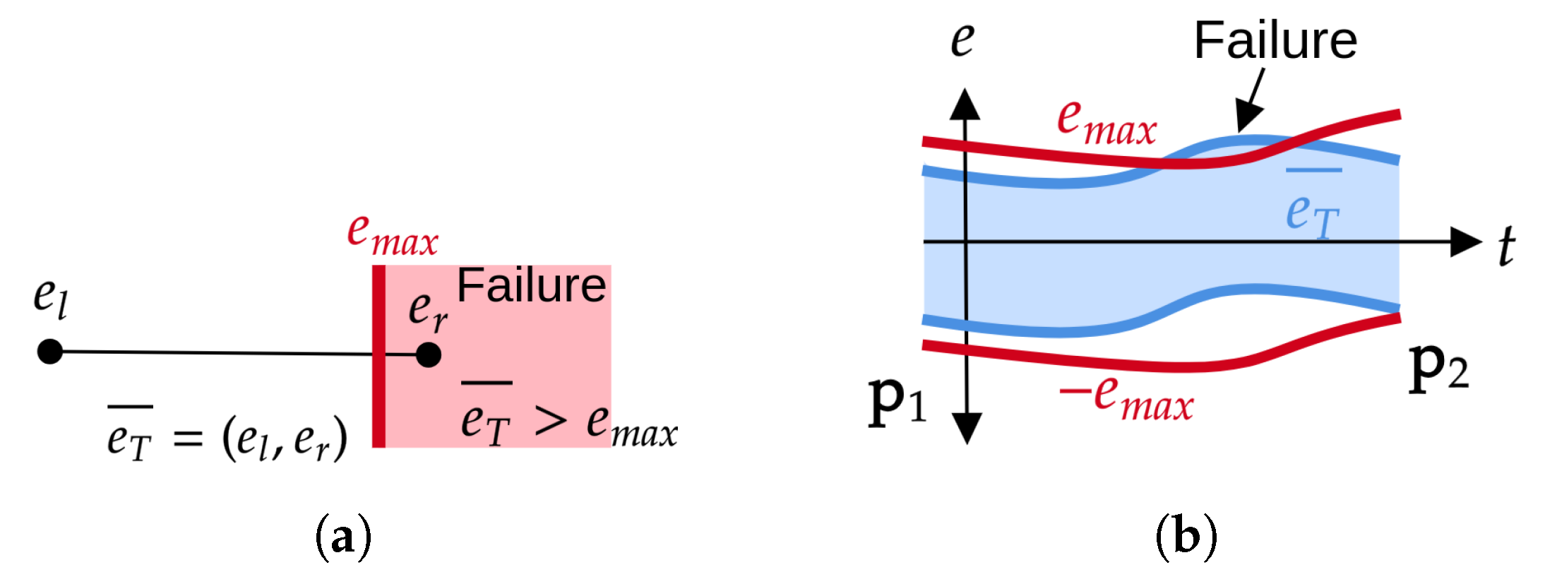
2. Interval Analysis and Reliability

Kinematic reliability refers to the probability that a mechanism will perform a specified motion within a certain error margin, denominated the kinematic error. Such motion errors can result from uncertainties in the geometric parameters, dimensional tolerances, assembly errors, thermal deformations, and clearances of the manipulator [16].

The innovation of the proposed interval reliability method lies in estimating the probability of kinematic failure linked to the maximum error defined as an interval, i.e., the interval errors are modeled as intervals that require the maximum and minimum limits. Compared to previous studies, this approach does not rely on prior knowledge of error probability densities [1,5,6,7,17] or the possibility distributions defined as the membership function of fuzzy errors required in the fuzzy methods [9]. Therefore, the interval method permits assessment based on a more straightforward description of errors compared to probabilistic and fuzzy methods.

The sources of kinematic error (clearances or dimensional tolerances) can be modeled as a set of n intervals that can be grouped into the vector $\overline{\mathit{\lambda }}=({\mathit{\lambda }}_l,{\mathit{\lambda }}_r)$, where ${\mathit{\lambda }}_l=\left[\begin{array}{ccc}{\lambda }_{l1}& \dots & {\lambda }_{ln}\end{array}\right]$ is the lower limit and ${\mathit{\lambda }}_r=\left[\begin{array}{ccc}{\lambda }_{r1}& \dots & {\lambda }_{rn}\end{array}\right]$ is the upper limit. The kinematic error can be denoted as $e_T=f\left(\mathit{\lambda }\right)$ and it can be computed based on the mapping error approach $f\left(\mathit{\lambda }\right)$ that determines the errors of the end-effector based on the kinematic model of the manipulator; $f\left(\mathit{\lambda }\right)$ is a kinematic model that quantifies the total kinematic error at the end-effector produced by $\mathit{\lambda }$. It is important to note that the kinematic error, $e_T$, can account for either the orientation error $e_T\left(\mathit{\lambda }\right)=\parallel \delta {\mathbf{p}}_r\parallel$ or the translational error $e_T\left(\mathit{\lambda }\right)=\parallel \delta {\mathbf{p}}_t\parallel$ separately, where $\parallel .\parallel$ denotes the vector magnitude, with ${\mathbf{p}}_t$ and ${\mathbf{p}}_r$ being the vectors of the translational error and orientation error, respectively.

The performance function $g\left(\mathit{\lambda }\right)$ is defined as the difference between a maximum allowable error ($e_{max}$) and the actual kinematic error resulting from uncertainties in the manipulator ($e_T\left(\mathit{\lambda }\right)$); thus,

$$g\left(\mathit{\lambda }\right)=e_{max}-e_T\left(\mathit{\lambda }\right)$$

(1)

The present work considers the errors as intervals $\overline{\mathit{\lambda }}$.

A two-dimensional performance function is considered $g\left(\overline{\mathit{\lambda }}\right)=g({\overline{\lambda }}_1,{\overline{\lambda }}_2)$ to illustrate the present approach. A failure occurs if the kinematic error $e_T\left(\overline{\mathit{\lambda }}\right)$ exceeds the admissible error; thus, $g\left(\overline{\mathit{\lambda }}\right)<0$. Consider a two-dimensional plane formed by the interval variables ${\overline{\lambda }}_1=({\lambda }_{1l},{\lambda }_{1r})$ and ${\overline{\lambda }}_2=({\lambda }_{2l},{\lambda }_{2r})$, as presented in Figure 1a. The curve $g\left(\mathit{\lambda }\right)$ splits the rectangular area of the variable space into two regions: a safe area and a fail area. The total rectangular area is defined as $A_{total}=({\lambda }_{1r}-{\lambda }_{1l})({\lambda }_{2r}-{\lambda }_{2l})$; moreover, the possibility that a failure occurs ($p_f$) can be quantified as the quotient of the failure area $A_{fail}$ and $A_{total}$; thus,

$$p_f={\displaystyle \frac{A_{fail}}{A_{total}}}$$

(2)

where $p_f$ quantifies the percentage rate at which the internal error exceeds the admissible error limit $|e_{max}|$. If ${\overline{e}}_T<\left|e_{max}\right|$, the failure index is zero; else, it is expressed as in Equation (2). As a result, the failure index is zero since the manipulator’s desired operating state requires end-effector error to not exceed the maximum limit. Likewise, the reliability can be defined by $R_{Int}$ as a percentage measure that indicates that the error will be contained within the maximum limit in the form

$$R_{Int}=1-p_f$$

(3)

Greater reliability is implied by $R_{Int}$ being closer to 1. Moreover, the failure area ($A_{total}$) can be determined by

$$A_{fail}=\int {\int }_{g\left(\lambda \right)<0}g({\lambda }_1,{\lambda }_2)d{\lambda }_{2}d{\lambda }_1$$

(4)

Therefore, the integral of Equation (4) should be numerically solved to estimate the possibility of failure. It is worth mentioning that the performance function $g\left(\mathit{\lambda }\right)$ depends on the nonlinear kinematic model of the manipulator that defines the positioning error.

Consider a n-dimensional case for the assessment of the reliability with n interval sources of errors defined as $\overline{\mathit{\lambda }}=\left[\begin{array}{ccc}{\overline{\lambda }}_1& \dots & {\overline{\lambda }}_n\end{array}\right]$. The new interval variable $\overline{\mathbf{z}}=(z_l,z_r)$ is defined and depends on the interval performance function $g\left(\overline{\mathit{\lambda }}\right)$ based on the definition of the performance function, $\overline{\mathbf{z}}=e_{max}-e_T\left(\overline{\mathit{\lambda }}\right)$. It is worth saying that the assessment of $\overline{\mathbf{z}}$ depends on the evaluation of the interval error $e_T\left(\overline{\mathit{\lambda }}\right)=(e_l,e_r)$.

The evaluation of $e_r$ and $e_l$ requires the resolution of an optimization problem in order to ascertain the maximum and minimum limits of the interval error generated by the interval parameters $\overline{\mathit{\lambda }}\in ({\mathit{\lambda }}_l,{\mathit{\lambda }}_r)$ in the form

$$\begin{array}{ccc}\hfill e_r=\underset{\mathit{\lambda }\in \overline{\mathit{\lambda }}}{max}{e}_T\left(\mathit{\lambda }\right)& \hfill & \hfill e_l=\underset{\mathit{\lambda }\in \overline{\mathit{\lambda }}}{min}{e}_T\left(\mathit{\lambda }\right)\end{array}$$

(5)

However, a failure can occur in the case that the interval error, $e_T$, exceeds an admissible limit $e_{max}$ (see Figure 2a). The failure measures the chance that the interval error will exceed the maximum error limit, $e_{max}$. According to Equation (1), a failure occurs when $\overline{\mathbf{z}}<0$, as presented in Figure 1b. The failure area $A_{fail}$ and the total area $A_{total}$ of Equation (4) correspond to the expressions of Equation (5), where $A_{fail}=e_r-e_{max}$ and $A_{total}=e_r$. Thus, the interval reliability is computed with the following expressions:

$$R_{Int}=1-{\displaystyle \frac{e_r-e_{max}}{e_r}}$$

(6)

The reliability is analyzed along the end-effector trajectory. Therefore, the interval error ${\overline{e}}_T$ is computed for the analyzed motion, and then, the reliability is assessed, as presented in Figure 2b. When the interval error surpasses the upper limit on errors, i.e., if the interval error surpasses $|e_{max}|$, it fails. Otherwise, if the interval error is less than $|e_{max}|$, it is contained within the permissible area (see Figure 2b); thus, $R_{Int}=1$. The cases in Figure 2 summarize the interpretation and practical application of the proposed interval reliability $R_{Int}$.

The flowchart in Figure 3 demonstrates the algorithm used to calculate the interval kinematic reliability. The computation of the interval reliability demands the minimization of a nonlinear, continuous function based on the kinematic model of the manipulator according to Equation (5). The application of evolutionary algorithms has demonstrated advantages over other techniques in engineering optimization problems [18]. Specifically, differential evolution (DE) has an advantage over genetic algorithm (GA) and particle swarm optimization (PSO) to solve this kind of optimization problem according to Kachitvichyanukul [19]. Thus, the differential evolution (DE) algorithm is used to determine the maximum limits $e_r$ of the interval error of ${\overline{e}}_T$ according to Equation (5). A set of candidate solutions ${\mathit{\lambda }}_c$ is first generated using DE operators. The positioning error $e_T$ is then calculated using the mapping error model $f\left({\mathit{\lambda }}_c\right)$ for these candidates, and they are refined through multiple iterations until the stopping criteria are satisfied to obtain $e_r$. The process to compute the interval reliability $R_{Int}$ described above is performed along the end-effector trajectory between the points ${\mathbf{p}}_1$ and ${\mathbf{p}}_2$ with an increment of $\Delta \mathbf{p}$.

The dynamic analysis of the reliability depends on the dynamic model of the manipulators. Reliability analysis subjected to clearances [20] and dimensional tolerances [17] was performed based on probabilistic approaches. The proposed approach to analyze the interval kinematic reliability can also be applied to the dynamic analysis by computing the interval error based on the dynamic modeling, i.e., considering the positioning error computed using the dynamic model instead of the error based on the kinematic model.

3. Case Studies

This section investigates how joint clearance and dimensional tolerances affect the kinematic reliability of manipulators using the interval reliability approach. First, a 3R serial manipulator with joint clearances is analyzed. Then, a Delta parallel manipulator with dimensional tolerances is analyzed.

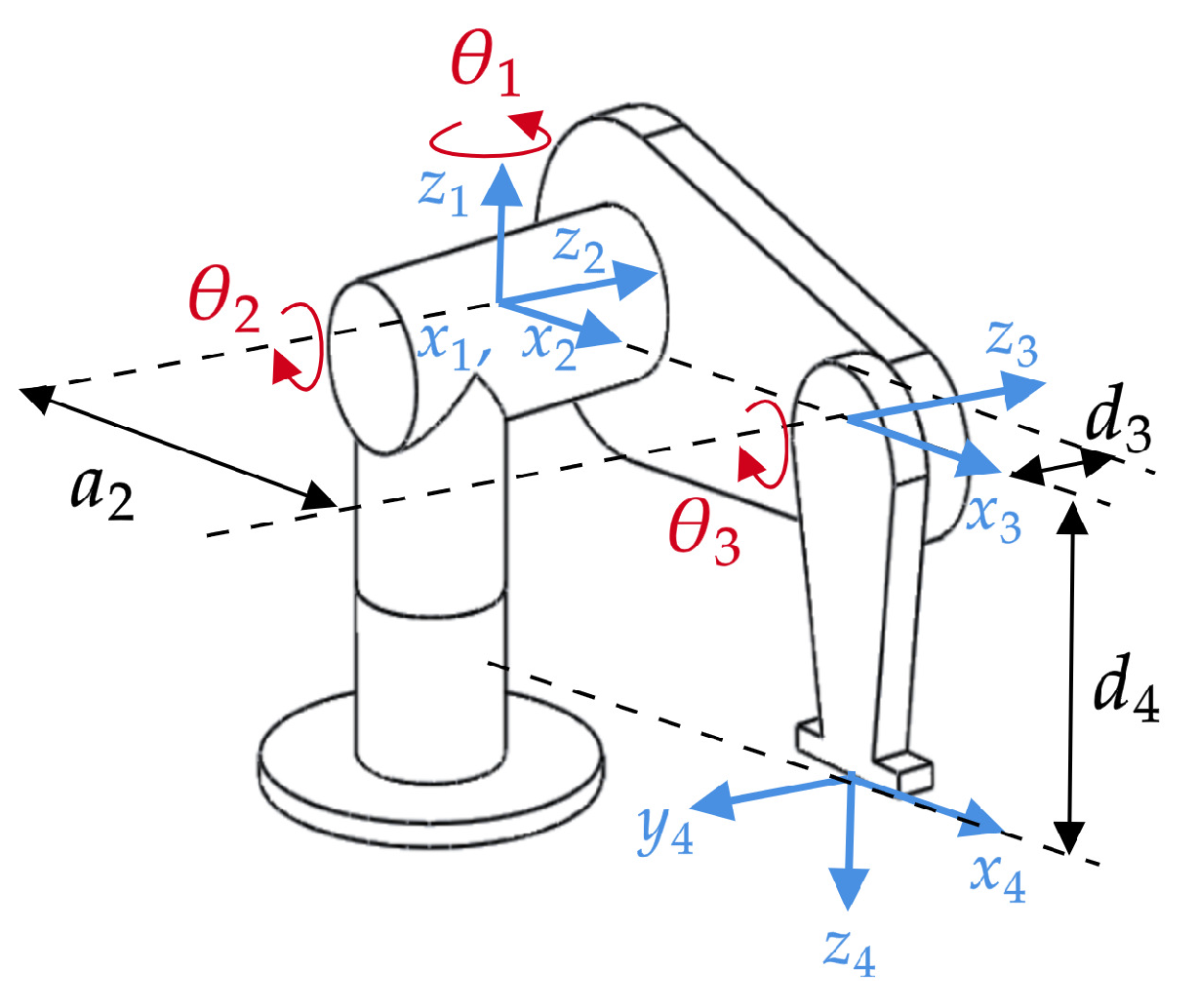
3.1. 3R Serial Manipulator Subjected to Clearances

The relationship between the axisymmetric joint clearance [21] and the interval parameters defines it. Thus, developing an error mapping technique may determine the positioning error on the end-effector caused by the joint clearances. This specific approach is formulated to compute the interval kinematic reliability.

Joint clearances cause errors inside the joints, according to the axisymmetric joint clearance model, which considers the revolute joint axis along the z-axis (see Figure 4 [21]). Therefore, the pose error at the local frame ($F_{i,j}$) is defined as the error screw $\delta {\mathbf{e}}_{i,j}$ given by

$$\delta {\mathbf{e}}_{i,j}={\left[\begin{array}{cc}\delta {\mathbf{r}}_{i,j}& \delta {\mathbf{t}}_{i,j}\end{array}\right]}^T$$

(7)

where i is the index of the kinematic chain, j is the index of the joint in the respective ith kinematic chain, $\delta {\mathbf{r}}_{i,j}={\left[\begin{array}{ccc}\delta r_{i,j,x}& \delta r_{i,j,y}& \delta r_{i,j,z}\end{array}\right]}^T$ is the orientation error, and $\delta {\mathbf{t}}_{i,j}={\left[\begin{array}{ccc}\delta t_{i,j,x}& \delta t_{i,j,y}& \delta t_{i,j,z}\end{array}\right]}^T$ is the translational error, as modeled in Figure 4.

Consequently, the components of the error screw $\delta {\mathbf{e}}_{i,j}$ of Equation (7) can be formulated as

$$\begin{array}{ccc}\hfill & \left\{\begin{array}{cc}\hfill \delta r_{i,j,x}& =\Delta {\beta }_{i,j,xy}cos\left({\gamma }_i\right)\hfill \\ \hfill \delta r_{i,j,y}& =\Delta {\beta }_{i,j,xy}sin\left({\gamma }_i\right)\hfill \\ \hfill \delta r_{i,j,z}& =\Delta {\beta }_{i,j,z}\hfill \end{array}\right.\hfill & \hfill \left\{\begin{array}{cc}\hfill \delta t_{i,jx}& =\Delta b_{i,j,xy}cos\left({\gamma }_i\right)\hfill \\ \hfill \delta t_{i,jx}& =\Delta b_{i,j,xy}sin\left({\gamma }_i\right)\hfill \\ \hfill \delta t_{i,jz}& =\Delta b_{i,j,z}\hfill \end{array}\right.\end{array}$$

(8)

with $0\le {\gamma }_{i,j}\le 2\pi$. The vector that joins the parameters of a joint clearance is defined as $\mathit{\lambda }=\left[\begin{array}{ccccc}{\mathit{\lambda }}_{i,1}& {\mathit{\lambda }}_{i,2}& \dots {\mathit{\lambda }}_{i,j}& \dots & {\mathit{\lambda }}_{n_i,n_j}\end{array}\right]$, where $j=1,\dots ,n_j$, $n_j$ is the number of joints of the ith kinematic chain, and ${\mathit{\lambda }}_{i,j}$ are the parameters of the jth joint clearance: ${\mathit{\lambda }}_{i,j}=\left[\begin{array}{ccccc}\Delta {\beta }_{j,z}& \Delta {\beta }_{j,xy}& {\gamma }_j& \Delta b_{j,xy}& \Delta b_{j,z}\end{array}\right]$. Additionally, the joint clearance’s characteristics can be described as intervals denoted by

$${\overline{\mathit{\lambda }}}_{i,j}=({\mathit{\lambda }}_{i,jl},{\mathit{\lambda }}_{i,jr})$$

(9)

with ${\mathit{\lambda }}_{i,jl}$ being the lower bound and ${\mathit{\lambda }}_{i,jr}$ the upper bound of the joint clearance parameters. The interval joint clearance error is obtained by applying the definition of Equations (7)–(9); thus, ${\overline{\delta \mathbf{e}}}_{i,j}$.

The end-effector’s pose is determined using the Denavit–Hartenberg method while considering no clearances. As a result, the definition of the homogeneous transformation matrix, ${\mathbf{S}}_{i,j}$, is

$${\mathbf{S}}_{i,j}=\left[\begin{array}{cc}{\mathbf{R}}_{i,j}& {\mathbf{t}}_{i,j}\\ {\mathbf{0}}_{1\times 3}& 1\end{array}\right]$$

(10)

with $i=1,\dots ,m$ and $j=1,\dots ,n_{i,f}$, respectively; m is the number of kinematic chains (for a single kinematic chain $m=1$), and $n_{i,f}$ is the total number of frames. ${\mathbf{S}}_{i,j}$ represents the transformation matrix from the frame ${\mathbf{F}}_{i,j}$ to the frame ${\mathbf{F}}_{i,j+1}$, ${\mathbf{R}}_{i,j}$ is the 3 × 3 rotation matrix and ${\mathbf{t}}_{i,j}={\left[\begin{array}{ccc}{x}_{i,j}& y_{i,j}& z_{i,j}\end{array}\right]}^T$ the translation 3 × 1 vector. The pose of the end-effector related to the ith kinematic chain, ${\mathbf{P}}_i$, is defined as

$${\mathbf{P}}_i=\prod _{j=1}^{n_{j,f}}{\mathbf{S}}_{i,j}$$

(11)

Nevertheless, taking into account the joint clearances, the end-effector’s posture, ${\mathbf{P}}_i^{\prime }$, will not be equal to the pose ${\mathbf{P}}_i$ presented in Equation (11). The adjoint map transformation matrix of ${\mathbf{S}}_{i,j}$ maps the error screw onto the end-effector at a specific pose, as presented in Equation (12):

$$adj\left({\mathbf{S}}_{i,j}\right)=\left[\begin{array}{cc}{\mathbf{R}}_{i,j}& {\mathbf{0}}_{3\times 3}\\ {\mathbf{T}}_{i,j}{\mathbf{R}}_{i,j}& {\mathbf{R}}_{i,j}\end{array}\right]$$

(12)

where ${\mathbf{T}}_{i,j}=\left[\begin{array}{ccc}0& -z_{i,j}& y_{i,j}\\ z_{i,j}& 0& -x_{i,j}\\ -y_{i,j}& x_{i,j}& 0\end{array}\right]$ is the skew-symmetric matrix of the vector ${\mathbf{t}}_{i,j}$. ${\mathbf{t}}_{i,j}$ and ${\mathbf{R}}_{i,j}$ can be extracted from the transformation matrix of Equation (10). Moreover, the adjoint of the inverse transformation matrix, $adj{\left({\mathbf{S}}_{i,j}\right)}^{-1}$, permits the expression of screws at the frame ${\mathbf{F}}_{i,j+1}$ from ${\mathbf{F}}_{i,j}$. Consequently, the end-effector’s pose error while taking into account all joint clearances can be written as

$$\overline{\delta \mathbf{p}}={\mathbf{M}}_i{\overline{\delta \mathbf{e}}}_i={\left[\begin{array}{cc}{\overline{\delta \mathbf{p}}}_r& {\overline{\delta \mathbf{p}}}_t\end{array}\right]}^T$$

(13)

where ${\mathbf{M}}_i=\left[\begin{array}{c}{\mathbf{M}}_{i,1}\cdots {\mathbf{M}}_{i,ni}\end{array}\right]$, $\delta {\mathbf{e}}_i=\left[\begin{array}{c}{\overline{\delta \mathbf{e}}}_{i,1}^T\cdots {\overline{\delta \mathbf{e}}}_{i,n_i}^T\end{array}\right]$.

${\mathbf{M}}_{i,j}={\displaystyle \prod _{l=1}^{n_{i,f}}}\left({\mathbf{N}}_{i,l}\right){\displaystyle \prod _{k=n_{i,f}}^{j+1}}\left(adj{\left({\mathbf{S}}_{i,k}\right)}^{-1}\right)$, and ${\overline{\delta \mathbf{p}}}_r$ and ${\overline{\delta \mathbf{p}}}_t$ are the end-effector’s translational error and orientation, respectively. Moreover, ${\mathbf{N}}_{i,j}=\left[\begin{array}{cc}{\mathbf{R}}_{i,j}& {\mathbf{0}}_{3\times 3}\\ {\mathbf{0}}_{3\times 3}& {\mathbf{R}}_{i,j}\end{array}\right]$ maps the orientation error and the translational error from the frame ${\mathbf{F}}_{i,P}$ to the frame ${\mathbf{F}}_{i,1}$.

The error mapping of Equations (7)–(13) can be used to evaluate the error at the end-effector, which is obtained based on Equation (13). The error, $e_T$, can take into account in the orientation error ($e_T=\left|\right|\delta {\mathbf{p}}_r\left|\right|$) and the translational error ($e_T=\left|\right|\delta {\mathbf{p}}_t\left|\right|$) separately, with $\left|\right|.\left|\right|$ being the magnitude of the vector. The parameters of the joint clearances are defined as an interval: ${\overline{\mathit{\lambda }}}_{i,j}=\left[\begin{array}{ccccc}{\overline{\Delta \beta }}_{j,z}& {\overline{\Delta \beta }}_{j,xy}& {\overline{\gamma }}_j& {\overline{\Delta b}}_{j,xy}& {\overline{\Delta b}}_{j,z}\end{array}\right]$. Consequently, the end-effector error will also be an interval output, where $e_T$ is defined as an interval ${\overline{e}}_T=(e_l,e_r)$.

Figure 5 presents the 3R manipulator case study, and

Table 1. D-H parameters.

j	${\mathit{\alpha }}_{\mathit{j}-1}$	${\mathit{a}}_{\mathit{j}-1}$	${\mathit{d}}_{\mathit{j}}$	${\mathit{\theta }}_{\mathit{j}}$
1	0	0	0	${\theta }_1$
2	$-{90}^{\circ }$	0	0	${\theta }_2$
3	0	$a_2$	$d_3$	${\theta }_3$
4	$-{90}^{\circ }$	0	$d_4$	0

lists its D-H parameters, with the error mapping, $i=1$ and $j=1,\dots ,3$. Furthermore, the link lengths are specified as $a_2$ = 0.15 m, $d_3$ = 0.01 m, and $d_4$ = 0.10 m, and the rotational joints are bounded in the following form: $-{100}^{\circ }\le {\theta }_1\le {90}^{\circ }$, $-{90}^{\circ }\le {\theta }_2\le {45}^{\circ }$, and $-{90}^{\circ }\le {\theta }_3\le {90}^{\circ }$.

3.1.1. Application of the Interval Approach

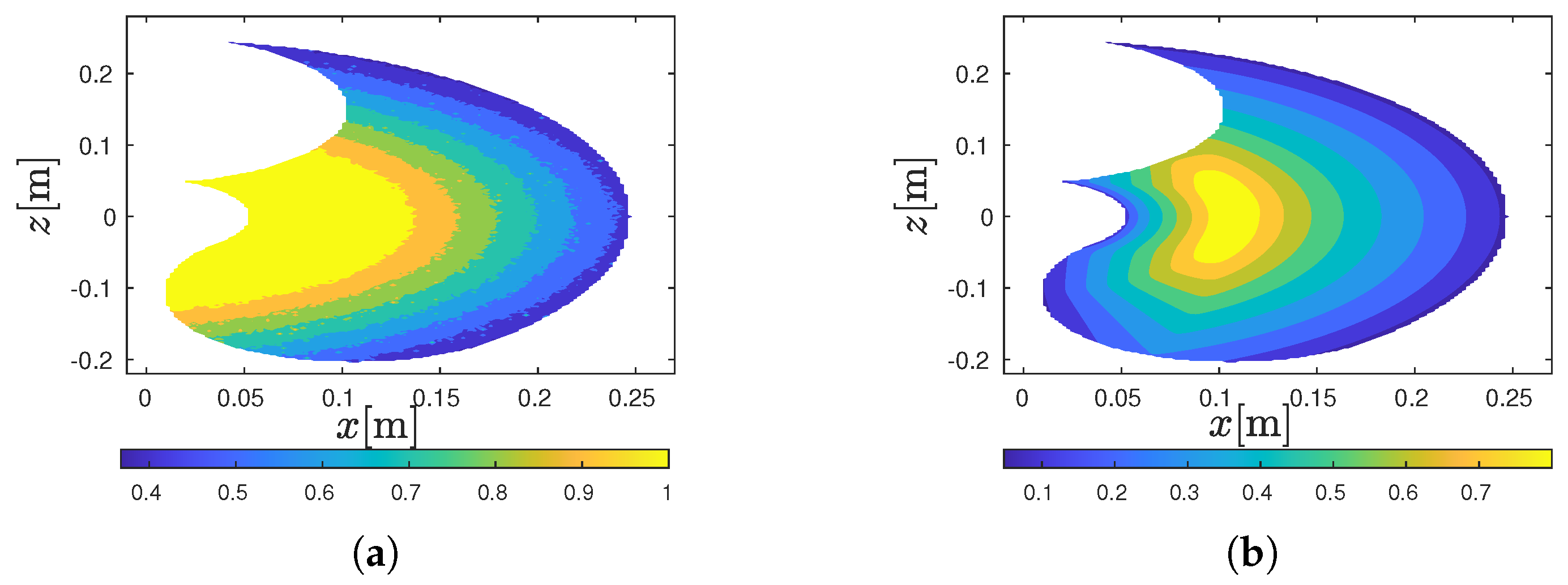
The interval kinematic reliability approach in Figure 3 is applied to the 3R manipulator of Figure 5. The joint clearance parameters are first specified as intervals: ${\overline{\Delta \beta }}_{xy}={(0,0.1)}^{\circ }$, ${\overline{\Delta \beta }}_z={(0,0.05)}^{\circ }$, ${\overline{\Delta b}}_{xy}=$$(0,1)\times {10}^{-4}$m, ${\overline{\Delta b}}_z=$$(0,1)\times {10}^{-4}$m, and $\overline{\gamma }={(0,360)}^{\circ }$. Moreover, no clearance is included around the z-axis (joint angles); thus, ${\beta }_z=0$. The translational error is examined in the present analysis, thus $e_T=\left|\right|\delta {\mathbf{p}}_t\left|\right|$; this error was computed based on the error mapping approach of Equation (13). The admissible error limit $e_{max}$ = $1\times {10}^{-3}$ m is used to evaluate the kinematic reliability. The joint clearance used in this paper is considered with tolerance zone h6 to precision mechanical adjustment for shafts with diameters between 10 and 18 mm. It should be noted that link parameters and joint clearance tolerances should be defined in the robot project design considering the mechanical manufacturing process.

This optimization problem (Equation (5)) to evaluate the interval error ${\overline{e}}_T=(e_l,e_r)$ was solved by using the differential evolution (DE) algorithm in [22]. The DE algorithm was used with the following parameters: a population size of 8 per variable, 40 generations, a perturbation rate of 0.8, a crossover probability rate of 0.8, and a mutation mechanism based on the DE/rand/1/bin approach.

3.1.2. Results

For this case study, the joint clearance parameters are also defined as normal random variables to assess the probabilistic approaches to assess the reliability: ($\theta )=\mu +\sigma \xi (\theta )$ with $\mu$ being the mean, $sigma$ the standard deviation, $\xi \left(\theta \right)$ being a unit normal random variable, and $\theta$ representing a random process. Thus, ${\Delta \beta }_{xy}\left(\theta \right)=0.0500+0.0333\xi {\left(\theta \right)}^{\circ }$, $\Delta {\beta }_z\left(\theta \right)$ = 0.0025 + 0.0008$\xi {\left(\theta \right)}^{\circ }$, $\Delta b_{xy}\left(\theta \right)=$$5\times {10}^{-5}$ + $3.3\times {10}^{-5}$$\xi \left(\theta \right)$ m, $\Delta b_z\left(theta\right)=$$5\times {10}^{-5}$ + $3.3\times {10}^{-5}$$\xi \left(\theta \right)$ m, and $\gamma \left(\theta \right)$ = 180 + 120$\xi {\left(\theta \right)}^{\circ }$. The normal random variables defined above have an equivalent dispersion of interval parameters, i.e., $\overline{\lambda }=(\mu -3\sigma ,\mu +3\sigma )$.

The proposed interval approach is initially compared to the Monte Carlo simulation, a well-known probabilistic approach, according to Appendix A. The performance function $g\left(\mathit{\lambda }\right)$ of Equation (1) is computed at the Cartesian positioning of the end-effector $\mathbf{p}={\left[\begin{array}{ccc}0.2& 0& 0\end{array}\right]}^T$ that corresponds to position ($b)$ of the workspace in Figure 6a. The interval reliability is computed using Equation (6), thus $R_{Int}$ = 0.7570; this corresponds to the possibility that the interval performance function is less than zero, i.e., it expresses the chance of interval error $\overline{\mathbf{e}}$ being more than the maximum admissible error $e_{max}$ (see Figure 6b) produced by the interval parameters of the clearances $\overline{\mathit{\lambda }}$. The probability density function (PDF) was also estimated based on the results obtained by using the Monte Carlo simulation (MCS) (see Figure 6b). The MCS estimates the probability of the error exceeding $e_{max}$, i.e., $g\left(\mathit{\lambda }\right)<0$; thus, the reliability is obtained as $R_{MCS}=$ 0.9999. Although the probability of the performance $g\left(\mathit{\lambda }\right)<0$ is almost null for this case study, the interval reliability $R_{Int}$ indicates that there is a possibility of this event occurring (see Figure 6b).

Then, the error of the end-effector and the reliability are examined for six different end-effector positions within the workspace according to Figure 6a. The outputs for the reliability are presented in

Table 2. Reliability outputs over workspace of the 3R manipulator.

	$\overline{\mathbf{e}}$	$\mathit{e}\left(\mathit{\theta }\right)$			${\mathit{R}}_{\mathit{Int}}$	${\mathit{R}}_{\mathit{MCS}}$	${\mathit{n}}_{\mathit{Int}}$	${\mathit{n}}_{\mathit{MCS}}$
	$({\mathit{e}}_{\mathit{l}},{\mathit{e}}_{\mathit{r}})$	${\mathit{\mu }}_{\mathit{e}}$	${\mathit{\sigma }}_{\mathit{e}}$	max
(a)	(0, 0.0012)	$3.2397\times {10}^{-4}$	$1.4202\times {10}^{-4}$	0.0011	1.0000	1.0000	5997	$1\times {10}^{-6}$
(b)	(0, 0.0020)	$5.2507\times {10}^{-4}$	$2.4602\times {10}^{-4}$	0.0017	0.7600	0.9999	5998	$1\times {10}^{-6}$
(c)	(0, 0.0021)	$5.5394\times {10}^{-4}$	$2.7086\times {10}^{-4}$	0.0019	0.7058	0.9990	5998	$1\times {10}^{-6}$
(d)	(0, 0.0022)	$5.8687\times {10}^{-4}$	$2.8855\times {10}^{-4}$	0.0020	0.6809	0.9973	5998	$1\times {10}^{-6}$
(e)	(0, 0.0021)	$5.6810\times {10}^{-4}$	$2.6659\times {10}^{-4}$	0.0019	0.7129	0.9990	4440	$1\times {10}^{-6}$
(f)	(0, 0.0014)	$3.8376\times {10}^{-4}$	$1.6366\times {10}^{-4}$	0.0013	1.0000	1.0000	5998	$1\times {10}^{-6}$

. For the interval approach, the error ${\overline{e}}_T=(e_l,e_r)$ is quantified according to Equation (5). Moreover, the interval reliability $R_{Int}$ is also evaluated. For the MCS, the error of the end-effector $e\left(\theta \right)$ is quantified by its mean ${\mu }_e$, standard deviation ${\sigma }_e$, and maximum value max$\left(e\right(\theta \left)\right)$. The reliability $R_{MSC}$ assesses the probabilistic reliability. One can observe a similar result for the maximum value of the error using both approaches ($e_r$ and $max\left(e\right(\theta \left)\right)$). Nevertheless, a sensible difference between the outputs obtained is observed using both approaches ($R_{Int}$ and $R_{MCS}$); this is produced because of the low probability of the error reaching high values. This underestimation produces low outputs for the probability of failure, and therefore, overestimates the reliability using MCS ($R_{MCS}$) compared to the reliability using the interval approach $R_{Int}$. It is worth mentioning that the concept of interval reliability is directly linked to the interval error ${\overline{e}}_T$, not to the probability of error $e\left(\theta \right)$. For this reason, the interpretation of the results and values of the outputs is different. Moreover, the computational cost of the methods was evaluated by assessing how many times the mapping error was required to estimate the reliability, as presented in Table 2, where $n_{Int}$ and $n_{MCS}$ represent the times that the mapping error was computed using the interval method and the Monte Carlo simulation, respectively. One can observe that the interval method demands the computation of the mapping error fewer times using the interval method than the Monte Carlo simulation.

Then, the end-effector’s error is calculated for a particular workspace trajectory $\mathbf{p}\left(t\right)$. Initially, the Cartesian trajectory of the end-effector is considered in this analysis, as presented in Figure 7a, as a straight path. Following that, the end-effector is mapped to the error caused by the joint clearances; thus, the interval error of the end-effector is computed for the x, y, and z axes. One can observe that the interval error varies during the motion, i.e., the width of the interval error changes during the motion, as reported in Figure 7b–d. The error model can be validated using the same procedure as in [23] to obtain experimental measurements of joint clearances and end-effector error.

Moreover, the Cartesian trajectory of the end-effector in Figure 7a was used to compute the reliability. First, the interval error ${\overline{e}}_T$ was computed for this analysis according to Equation (5), with the results shown in Figure 8a. Three different limits for the error were defined to evaluate the reliability along the motion: $e_{max1}$ = $2\times {10}^{-3}$ m, $e_{max2}$ = $1.75\times {10}^{-3}$ m, and $e_{max3}$ = $1.5\times {10}^{-3}$ m. The reliability along the trajectory considering these three different error limits was computed according to Equation (3) for these different error limits. One can observe that reducing the admissible error limit ($e_{max}$) also implies a decrease in reliability. Moreover, the reliability also varies during the motion and depends on the width of the interval error, as shown in the computed results in Figure 8b.

The kinematic reliability can also be evaluated over the workspace with y = 0, as shown in Figure 9a. The reliability, $R_{Int}$, drops near the workspace’s outside boundaries; the manipulator linkages are extended in these positions. The reduction in reliability $R_{Int}$ is produced by increasing the error at the workspace’s outer borders. The workspace bounds on the left side are the poses wherein the links are retracted. Therefore, the error decreases, and $R_{Int}$ increases. In addition, one can observe a positive relationship between reliability (see Figure 9a) and kinematic dexterity calculated using the Jacobian matrix’s inverse condition number $1/\kappa \left(\mathbf{J}\right)$ (see Figure 9b) for the poses wherein the links are extended; i.e., $R_{Int}$ decreases and also the kinematic dexterity ($1/\kappa \left(\mathbf{J}\right)$) decreases. Nevertheless, this behavior is not shown when reducing the error for the postures in which the linkages are retracted.

3.2. Delta Parallel Manipulator

The interval reliability is applied to the Delta parallel manipulators subjected to dimensional uncertainties. Moreover, the interval approach is compared to the first-order reliability method (FORM) that has already been used for the reliability analysis of manipulators [1].

The Delta parallel manipulator of Figure 10a is composed of three symmetrical kinematic chains that join the moving platform (see Figure 10a) and fixed base (see Figure 10a). The frames $\left\{B\right\}$ and $\left\{P\right\}$ are located at the fixed base (see Figure 10b) and the moving platform (see Figure 10c), respectively. Each kinematic chain has the configuration $\underline{R}UU$, where $\underline{R}$ represents the active rotational joint located at point $B_i$ on the fixed base. This active joint is defined by the angle ${\theta }_i$ for $i=1,2,3$. The lower links, each with length $l_i$, are modeled as a four-bar parallelogram mechanism to ensure translational motion with a constant orientation in the moving platform. The forward kinematic solution utilized in this study follows the approach described in [24].

The frames $\left\{P\right\}$ and $\left\{B\right\}$ share the same orientation denoted by the constant orientation matrix ${}_P{}^B\mathbf{R}={\mathbf{I}}_3$. The vector of active joint variables is given by ${\left[\begin{array}{ccc}{\theta }_1& {\theta }_2& {\theta }_3\end{array}\right]}^T$. At the same time, the Cartesian position of the moving platform is represented as $\mathbf{p}={\left[\begin{array}{ccc}{p}_x& p_y& p_z\end{array}\right]}^T$. According to the kinematic modeling defined by [25], the following six parameters define the geometry of the manipulator: $s_{Pi}$, $w_{Pi}$, and $u_{Pi}$ define the geometry of the moving base; $w_{Bi}$ defines the fixed base; and $l_i$ and $L_i$ define the lengths of the lower and upper links, respectively, for $i=1,2,3$. For the present case study, the numerical values of these geometric parameters are defined in

Table 3. Geometric parameters of the Delta manipulator.

Parameter	${\mathit{S}}_{\mathit{Bi}}$	${\mathit{S}}_{\mathit{Pi}}$	${\mathit{L}}_{\mathit{i}}$	${\mathit{l}}_{\mathit{i}}$	${\mathit{w}}_{\mathit{Bi}}$	${\mathit{u}}_{\mathit{Bi}}$	${\mathit{w}}_{\mathit{Pi}}$	${\mathit{u}}_{\mathit{Pi}}$
Value [m]	0.567	0.076	0.524	1.244	0.164	0.327	0.022	0.044

.

3.2.1. Application of the Interval Approach

The interval reliability quantifies how the interval tolerances affect the Cartesian positioning error of the end-effector. The reliability algorithm of Figure 3 is applied for the Delta parallel manipulator considering the interval dimensional tolerance $\overline{\mathit{\lambda }}=\left[\begin{array}{ccc}{\overline{\delta l}}_1& \dots & {\overline{\delta l}}_6\end{array}\right]$ for the six geometric parameters of Table 3, with ${\overline{\delta l}}_i=(0,\delta l_r)$; i.e., every geometric parameter has an interval error of ${\overline{\delta l}}_i$ for $i=1,\dots ,6$. For this case study, the Delta interval dimensional tolerance was defined considering a low-cost laboratory-made robot with low dimensional accuracy of $\delta l_r$ = $1\times {10}^{-3}$ m.

The positioning error $e_T$ of the end-effector at position $\mathbf{p}$ is subjected to interval dimensional tolerances $\overline{\mathit{\lambda }}$ using Equation (14). The end-effector error ${\overline{e}}_T$ is stated by the difference of position $\mathbf{p}$ and the position under the interval parameters $\mathbf{p}\left(\overline{\mathit{\lambda }}\right)$, which is computed based on the forward kinematic model

$${\overline{e}}_T=\left|\right|\mathbf{p}-\mathbf{p}\left(\overline{\mathit{\lambda }}\right)\left|\right|$$

(14)

The optimization problem of Equation (5) to determine ${\overline{e}}_T=(e_l,e_r)$ based on the mapping model of Equation (14) is solved using differential evolution (DE) [22]. The population was fixed as 50 individuals, and a crossover probability rate of 0.8, perturbation rate of 0.8, and the DE/rand/1/bin mutation mechanism were used; the upper and lower limits for the search space are ${\mathit{\lambda }}_l$ and ${\mathit{\lambda }}_r$, respectively.

3.2.2. Results and Analysis

Figure 11 presents the workspace and the Cartesian positions of the end-effector over the plane $xz$ for $y=0$ m (see Figure 11a). This analysis considers six different end-effector positions over the workspace, as presented in Figure 11a. Moreover, the Cartesian trajectory $\mathbf{p}\left(t\right)$ (passing by the points ${\mathbf{p}}_G$, ${\mathbf{p}}_F$, and ${\mathbf{p}}_D$) of the end-effector to analyze the reliability is defined.

The interval reliability $R_{Int}$ is computed over the workspace as presented in Figure 11b for the maximum allowable error $e_{max}$ = $1\times {10}^{-3}$ m; the reliability, $R_{Int}$, decreases near the outer boundaries of the workspace, where the manipulator’s linkages are fully extended. This drop in $R_{Int}$ is caused by increased error at the workspace’s edges. Conversely, the error is reduced in the center region of the workspace, increasing $R_{Int}$. For this case study, a direct relationship between interval reliability (see Figure 11b) and kinematic dexterity ($1/\kappa \left(\mathbf{J}\right)$) of Figure 11c is also observed. For poses in the external border of the workspace, $R_{Int}$ and the kinematic dexterity decrease. However, in regions closer to the center of the workspace, these properties increase because the kinematic error on the end-effector is reduced, and the Jacobian matrix is far from the singular poses of the workspace’s external border.

Initially, the kinematic reliability subjected to the dimensional tolerances is computed by using the interval approach using the Monte Carlo simulation (see Appendix A), the first-order reliability method (FORM) (see Appendix B), and the interval approach to compare these three approaches. The random tolerances were defined in the following form: $\delta l\left(\theta \right)=\mu +\sigma \xi \left(\theta \right)$, with $\overline{\delta l}=(0,\mu +3\sigma )$; thus, $\mu$ = $0.25\times {10}^{-3}$m and $\sigma$ = $0.83\times {10}^{-4}$ m.

Table 4. Reliability outputs over workspace of the Delta parallel manipulator.

	${\mathit{R}}_{\mathit{Int}}$	${\mathit{R}}_{\mathit{MCS}}$	${\mathit{R}}_{\mathit{FORM}}$	${\mathit{n}}_{\mathit{Int}}$	${\mathit{n}}_{\mathit{MCS}}$	${\mathit{n}}_{\mathit{FORM}}$
(a)	0.8652	1.0000	1.0000	2215	100,000	117
(b)	0.5939	0.9987	0.9989	2407	100,000	156
(c)	0.5928	0.9985	0.9989	2401	100,000	156
(d)	0.7986	0.9999	0.9999	2409	100,000	91
(e)	0.7793	1.0000	1.0000	2412	100,000	260
(f)	0.7807	1.0000	1.0000	2031	100,000	260

shows the reliability outputs using the probabilistic methods (MCS and FORM) and the interval approach. First, the reliability using the probabilistic methods is quite similar ($R_{MCS}$ and $R_{FORM}$). The computational cost of the methods was evaluated by assessing how many times the mapping error was required to estimate the reliability. The MCS demands many samples $n_{MCS}$ to estimate the reliability accurately. Thus, the times that the mapping error of Equation (14) is required for MCS is greater than when using FORM ($n_{FORM}$). The interval approach exhibits an intermediate computational cost, according to $n_{Int}$, compared to MCS and FORM.

Figure 12 shows the interval reliability assessment along the Cartesian trajectory presented in Figure 11a. The behavior of the interval reliability, $R_{Int}$, follows the exact behavior of the kinematic dexterity based on the inverse conditional number of the Jacobian matrix ($1/\kappa \left(\mathbf{J}\right)$) for this specific trajectory (see Figure 12a).

Three different limits $\delta l_r$ for the dimensional tolerance ${\overline{\delta l}}_i=(0,\delta l_r)$ were defined to evaluate the reliability along the motion along the trajectory in Figure 11a: $\delta l_{r1}$ = $0.5\times {10}^{-3}$ m, $\delta l_{r2}$ = $1.0\times {10}^{-3}$ m, and $e_{max3}$ = $1.5\times {10}^{-3}$ m. The interval reliability along the trajectory considering these three definitions of the dimensional tolerances was computed using Equation (3). The increase in the dimensional tolerance limit ($\delta l_r$) implies a decrease in reliability, $R_{Int}$; see Figure 12b. One can observe that reliability $R_{Int}$ varies during the motion depending on the width of the interval dimensional tolerances.

4. Conclusions

This study proposes a novel method for utilizing the error interval definition to estimate manipulators’ kinematic reliability. This method can be used instead of considering joint clearance faults like random variables and replacing the probabilistic methods that are commonly used in the literature. Additionally, the error mapping technique, which accounts for the joint clearances of manipulators that are described as intervals, is used in the proposed methodology to quantify the kinematic dependability.

The effects of dimensional tolerances and clearance errors represented as intervals can be measured using kinematic reliability as an analysis criterion. The two case studies showed that the proposed interval approach permits the evaluation of the reliability of serial and parallel manipulators. Furthermore, no effect of joint clearance errors on the kinematic accuracy was demonstrated by the kinematic dexterity, based on the condition number of the Jacobian matrix. Additionally, the interval definition of error-based kinematic reliability makes it possible to calculate the percentage by which the error exceeds a tolerable bound. As a result, the reliability provides supplementary data for manipulator kinematic analysis.

The proposed interval reliability method is a complementary analysis approach that can help assess the kinematic performance of robotic manipulators. The interval method can convey additional information about the kinematic behavior of a manipulator subjected to interval errors based on reliability evaluation. In a practical application, the interval reliability method could be used in optimal kinematic design based on interval error sources; thus, the interval reliability criterion could be taken into account in the design of a manipulator.

In future work, the robust optimal robotic manipulators will be designed using a real analysis based on interval error. Moreover, the dynamic analysis of interval clearances will also be carried out.

References

1. Lara-Molina, F.A.; Dumur, D. Global performance criterion of robotic manipulator with clearances based on reliability. J. Braz. Soc. Mech. Sci. Eng. 2020, 42, 624. [Google Scholar] [CrossRef]
2. Zhan, Z.; Zhang, X.; Jian, Z.; Zhang, H. Error modelling and motion reliability analysis of a planar parallel manipulator with multiple uncertainties. Mech. Mach. Theory 2018, 124, 55–72. [Google Scholar] [CrossRef]
3. Cui, G.; Zhang, H.; Zhang, D.; Xu, F. Analysis of the kinematic accuracy reliability of a 3-DOF parallel robot manipulator. Int. J. Adv. Robot. Syst. 2015, 12, 15. [Google Scholar] [CrossRef]
4. Zhang, D.; Shen, S.; Wu, J.; Wang, F.; Han, X. Kinematic trajectory accuracy reliability analysis for industrial robots considering intercorrelations among multi-point positioning errors. Reliab. Eng. Syst. Saf. 2023, 229, 108808. [Google Scholar] [CrossRef]
5. Pandey, M.D.; Zhang, F. System reliability analysis of the robotic manipulator with random joint clearances. Mech. Mach. Theory 2012, 58, 137–152. [Google Scholar] [CrossRef]
6. Zhang, D.; Han, X. Kinematic reliability analysis of robotic manipulator. J. Mech. Des. 2020, 142, 44502. [Google Scholar] [CrossRef]
7. Zhang, J.; Du, X. Time-dependent reliability analysis for function generation mechanisms with random joint clearances. Mech. Mach. Theory 2015, 92, 184–199. [Google Scholar] [CrossRef]
8. Kim, J.; Song, W.J.; Kang, B.S. Stochastic approach to kinematic reliability of open-loop mechanism with dimensional tolerance. Appl. Math. Model. 2010, 34, 1225–1237. [Google Scholar] [CrossRef]
9. Lara-Molina, F.A.; Dumur, D. A fuzzy approach for the kinematic reliability assessment of robotic manipulators. Robotica 2021, 39, 2095–2109. [Google Scholar] [CrossRef]
10. Faes, M.; Moens, D. Recent trends in the modeling and quantification of non-probabilistic uncertainty. Arch. Comput. Methods Eng. 2020, 27, 633–671. [Google Scholar] [CrossRef]
11. Kang, R.; Zhang, Q.; Zeng, Z.; Zio, E.; Li, X. Measuring reliability under epistemic uncertainty: Review on non-probabilistic reliability metrics. Chin. J. Aeronaut. 2016, 29, 571–579. [Google Scholar] [CrossRef]
12. Nikolaidis, E.; Ghiocel, D.M.; Singhal, S. Engineering Design Reliability Handbook; CRC Press: Boca Raton, FL, USA, 2004. [Google Scholar]
13. Chang, Q.; Zhou, C.; Wei, P.; Zhang, Y.; Yue, Z. A new non-probabilistic time-dependent reliability model for mechanisms with interval uncertainties. Reliab. Eng. Syst. Saf. 2021, 215, 107771. [Google Scholar] [CrossRef]
14. Yang, C.; Lu, W.; Xia, Y. Positioning accuracy analysis of industrial robots based on non-probabilistic time-dependent reliability. IEEE Trans. Reliab. 2023, 73, 608–621. [Google Scholar] [CrossRef]
15. Tang, Z.; Peng, J.; Sun, J.; Meng, X. Non-probabilistic reliability analysis of robot accuracy under uncertain joint clearance. Machines 2022, 10, 917. [Google Scholar] [CrossRef]
16. Pritschow, G.; Eppler, C.; Garber, T. Influence of the dynamic stiffness on the accuracy of PKM. In Proceedings of the Chemnitz Parallel Kinematic Seminar, Chemnitz, Germany, 23–25 April 2002; pp. 313–333. [Google Scholar]
17. Rao, S.; Bhatti, P. Probabilistic approach to manipulator kinematics and dynamics. Reliab. Eng. Syst. Saf. 2001, 72, 47–58. [Google Scholar] [CrossRef]
18. Slowik, A.; Kwasnicka, H. Evolutionary algorithms and their applications to engineering problems. Neural Comput. Appl. 2020, 32, 12363–12379. [Google Scholar] [CrossRef]
19. Kachitvichyanukul, V. Comparison of three gorithms: GA, PSO, and DE. Ind. Eng. Manag. Syst. 2012, 11, 215–223. [Google Scholar]
20. Xiang, W.; Yan, S. Dynamic analysis of space robot manipulator considering clearance joint and parameter uncertainty: Modeling, analysis and quantification. Acta Astronaut. 2020, 169, 158–169. [Google Scholar] [CrossRef]
21. Meng, J.; Zhang, D.; Li, Z. Accuracy analysis of parallel manipulators with joint clearance. J. Mech. Des. 2009, 131, 11013. [Google Scholar] [CrossRef]
22. Storn, R.; Price, K. Differential evolution—A simple and efficient heuristic for global optimization over continuous spaces. J. Glob. Optim. 1997, 11, 341–359. [Google Scholar] [CrossRef]
23. Erkaya, S.; Uzmay, I. Experimental investigation of joint clearance effects on the dynamics of a slider-crank mechanism. Multibody Syst. Dyn. 2010, 24, 81–102. [Google Scholar] [CrossRef]
24. Williams, R.L.; Albus, J.S.; Bostelman, R.V. 3D Cable-Based Cartesian Metrology System. J. Robot. Syst. 2004, 21, 237–257. [Google Scholar] [CrossRef]
25. Williams, R.L., II. The Delta Parallel Robot: Kinematics Solutions. 2016. Available online: https://people.ohio.edu/williams/html/PDF/DeltaKin.pdf (accessed on 4 September 2024).
26. Rackwitz, R. Practical Probabilistic Approach to Design. In Bulletin No. 112; Comite European du Beton: Paris, France, 1976. [Google Scholar]
Figure 1. Interval reliability. (a) Variable space; (b) interval performance variable z ¯ .
Robotics 13 00155 g001
Figure 2. Interval reliability. (a) Failure condition; (b) failure during a motion.
Robotics 13 00155 g002
Figure 3. Flowchart of the interval kinematic reliability method.
Robotics 13 00155 g003
Figure 4. A standard joint clearance model [21]. (a) x y plane, (b) x z plane.
Robotics 13 00155 g004
Figure 5. 3R manipulator.
Robotics 13 00155 g005
Figure 6. Reliability assessment using the interval approach and the Monte Carlo simulation. (a) Usable workspace; (b) interval performance variable z ¯ and MCS.
Robotics 13 00155 g006
Figure 7. Cartesian trajectory and interval error for the case study in Figure 5. (a) Trajectory of the end-effector, (b) x-axis, (c) y-axis, (d) z-axis.
Robotics 13 00155 g007
Figure 8. Interval error and reliability. (a) Failure condition, (b) R I n t during a motion.
Robotics 13 00155 g008
Figure 9. Reliability and kinematic dexterity over workspace for the case study in Figure 5. (a) Interval reliability ( R I n t ), (b) 1 / κ ( J ) .
Robotics 13 00155 g009
Figure 10. Delta manipulator and its geometric parameters. (a) Delta manipulator; (b) fixed base; (c) moving platform.
Robotics 13 00155 g010
Figure 11. Workspace of the Delta manipulator. (a) Plane x z for y = 0 m; (b) R I n t over the workspace; (c) 1 / κ ( J ) over the workspace.
Robotics 13 00155 g011
Figure 12. Reliability and kinematic dexterity for the case study in Figure 10. (a) Reliability and 1 / κ ( J ) ; (b) reliability and δ l .
Robotics 13 00155 g012