1. Introduction
The analysis and development of control systems for autonomous vehicles has been a continuously active area of research. One of the key challenges for mobile devices lies in their capability to achieve a high level of autonomy. Accurate guidance, navigation, and control are of paramount importance for achieving autonomy. They basically rely on the performance of the robot’s localization system. Indeed, localization plays a fundamental role in the navigation of mobile ground robots, allowing them to learn their position and orientation in the environment [
1]. It is crucial for various applications, including autonomous exploration, path planning, and object manipulation.
To achieve accurate localization, sensor fusion techniques are commonly employed to integrate data from different sources and sensors. Among these techniques, odometry stands out; it is a widely adopted method of estimating the motion and position of a vehicle by combining data from the vehicle’s odometer (which relies on wheel revolutions), and kinematic models.
However, odometry has inherent limitations. It assumes that wheel revolutions directly correspond to linear displacement, neglecting factors such as wheel slippage, terrain variations, and mechanical imperfections. Consequently, odometry can accumulate errors over time. Such errors can be categorized into systematic and non-systematic errors [
2]. Systematic errors arise due to biases in the robot’s kinematic model, wheel size discrepancies, or misalignment between the sensors and the robot’s body. Non-systematic errors, on the other hand, are unpredictable and can occur during the robot’s operation, such as slippage on low-friction surfaces. Both types of errors contribute to the overall inaccuracy of odometry and hinder the robot’s precise localization.
Odometry calibration aims at identifying and correcting the kinematic parameters of the robot’s motion model to improve localization accuracy. By accurately calibrating the odometry system, systematic errors can be minimized, resulting in more reliable estimates of the robot’s position and orientation. Nevertheless, during the odometry calibration procedure, non-systematic errors, such as slippage, can introduce additional uncertainties and errors. Slippage occurs when the wheels lose traction with the ground surface, leading to inconsistent wheel revolutions and inaccurate odometry measurements. Addressing and reducing these non-systematic errors, including slippage, is crucial for achieving a reliable and accurate localization system.
1.1. Odometry Calibration Literature Review
Over the years, numerous studies have focused on odometry calibration techniques. Recently, a review article [
3] has been published on this topic, presenting a comparative survey of the existing techniques. The literature can be roughly categorized into three approaches [
4]:
- (i)
Offline One-Time Calibration (Before Use).
- (ii)
Online Calibration, separate from Localization.
- (iii)
Online Calibration Integrated into Robot Localization Algorithm.
Here, we briefly discuss the features of each approach.
1.1.1. Offline One-Time Calibration before Use
Papers falling into this area propose an offline calibration process that is performed once before deploying the robot, and typically involves predefined test paths or maneuvers to collect data for calibration. The work in [
5] introduced the pioneer method for odometry calibration, which served as the basis for subsequent studies. This method, for the first time, enabled the calibration of differential robot parameters by combining rotations and translations in a square path. The authors of [
6] further demonstrated that the path size influences the calibrated odometry accuracy, and proposed a 2 × 2 m square path for calibration. Since then, various approaches have emerged in the quest to identify the optimal calibration path. Researchers have explored different path designs and lengths to enhance the accuracy of calibrated odometry. These investigations have led to the introduction of alternative calibration methods and paths, such as the rotational motion-focused approach [
7], the distance-based approach utilizing three points [
8], and the bidirectional circular path test (BCPT) [
9], as an alternative to square paths, aiming to reduce the probability of slippage and minimize effort during the calibration process. Ivanjko et al. [
10] introduced a simplified calibration path consisting of straight-line motions and 180-degree rotations, offering a more straightforward approach with reduced space requirements. All of these methodologies, as exemplified in [
11], have demonstrated remarkable effectiveness. It is worth noting, however, that these calibration paths often necessitate substantial space, leading to interruptions in the robot’s regular usage. Moreover, conducting calibration tests in diverse environmental conditions, including various surfaces or terrains, poses significant challenges due to the extensive spatial requirements and difficulties in replicating real-world scenarios. These challenges highlight the need for calibration methods that can provide accurate results with minimal disruption to the robot’s regular activities.
1.1.2. Online Calibration Separate from Localization
To overcome the limitations of previous methods, researchers have developed Online Calibration methodologies that enable the calibration of robot kinematic parameters during normal usage. In [
12] odometry calibration is formulated as a linear problem, utilizing multiple calibration runs with different trajectories to compute an unbiased estimator. In [
13] a terminal iterative learning control (TILC) algorithm is employed, requiring only one calibration run but relying on the chosen trajectory for odometry accuracy. However, it is important to consider that these methods encounter challenges in the absence of continuous position measurements along the entire trajectory. They are susceptible to uncontrolled slippage phenomena, which can impact the calibration process. To enhance robustness against slippage, a significant number of calibration paths are often necessary.
1.1.3. Online Calibration Integrated into Robot Localization Algorithm
Another set of approaches integrates online calibration directly into the robot’s localization fusion algorithm. These methods continuously update the calibration parameters based on real-time sensor measurements and fusion algorithms, improving the localization accuracy during robot operation. Ref. [
14] presented a method that simultaneously calibrates odometry and extrinsic sensor parameters by leveraging the robot’s relative motion throughout the entire trajectory. The work in [
4] employed absolute localization systems and utilized the robot’s position over the entire trajectory, resulting in a more complex calibration procedure. Additionally, several Kalman Filter-based methods have been proposed for odometry calibration, as for example [
15,
16,
17] developed approaches that utilize Kalman filters and incorporate laser, DGPS, and inertial/magnetometer data, respectively. However, these approaches often require additional hardware, such as positioning systems for indoor environments like motion capture systems, and rarely provide direct position measurements as those offered by GPS systems for outdoor environments.
1.2. Paper Contribution and Organization
Motivated by the above considerations, in this work we present a novel online calibration method with enhanced robustness against slippage phenomena which is built on arbitrary paths commonly executed by robots during their operations. The proposed approach relies on an
active slippage compensation during odometry calibration, built on a slippage detection system, which disconnects data collection from encoders for odometry calibration while slippering, and in turn triggers an IMU-based motion reconstruction algorithm to estimate and correct position data during slipping periods for odometry calibration. The basic idea is to maintain the original approach of [
12], which is applied to an indoor differential robot, utilizing only proprioceptive sensor data, and eliminating the acquisition from signals affected by slippage when the traditional kinematic model becomes invalid. As long as slipping is detected, motion reconstruction is based on the only correct data available, namely IMU data. It is worth remarking that IMU-based short-time motion reconstruction is recently very active for the wide emerging applications (apart robotics), e.g., medicine, sports, rockfalls, snow avalanches and other risky environments where motion detection can be exploited for incipient disaster prediction [
18,
19]. The aim of the proposed methodology is to provide an online calibration algorithm that detects early slippage and effectively addresses its impact by utilizing gyroscopes and IMU, without the need for direct position measurements that may not always be available. A peculiar feature of the proposed algorithm is that it does not require a prescribed reference trajectory so that it can be run periodically to check eventual time variations of the kinematic matrix.
The rest of this paper is organized as follows.
Section 2 theoretically formalizes the addressed problem.
Section 3 presents our novel online calibration method with enhanced robustness against slippage phenomena. Exhaustive numerical simulations are reported in
Section 4 to evaluate and validate its performance in different scenarios. Finally, concluding remarks are summarized in
Section 5.
3. Online Calibration in Presence of Slippage
Inspired by the Least-Squares calibration approach [
12] briefly summarized in
Appendix A, we propose a methodology that takes into consideration slippage phenomena that may occur during the calibration process, making the analysis in [
12] no longer valid. As in [
12], we consider the following assumptions:
- A1.
The path is divided into N steps.
- A2.
Each step is completed in a fixed time .
- A3.
We have a constant , in each steps.
- A4.
The initial and final poses are known from measurements (for instance, by using exteroceptive sensors at the start and the end of the considered trajectory).
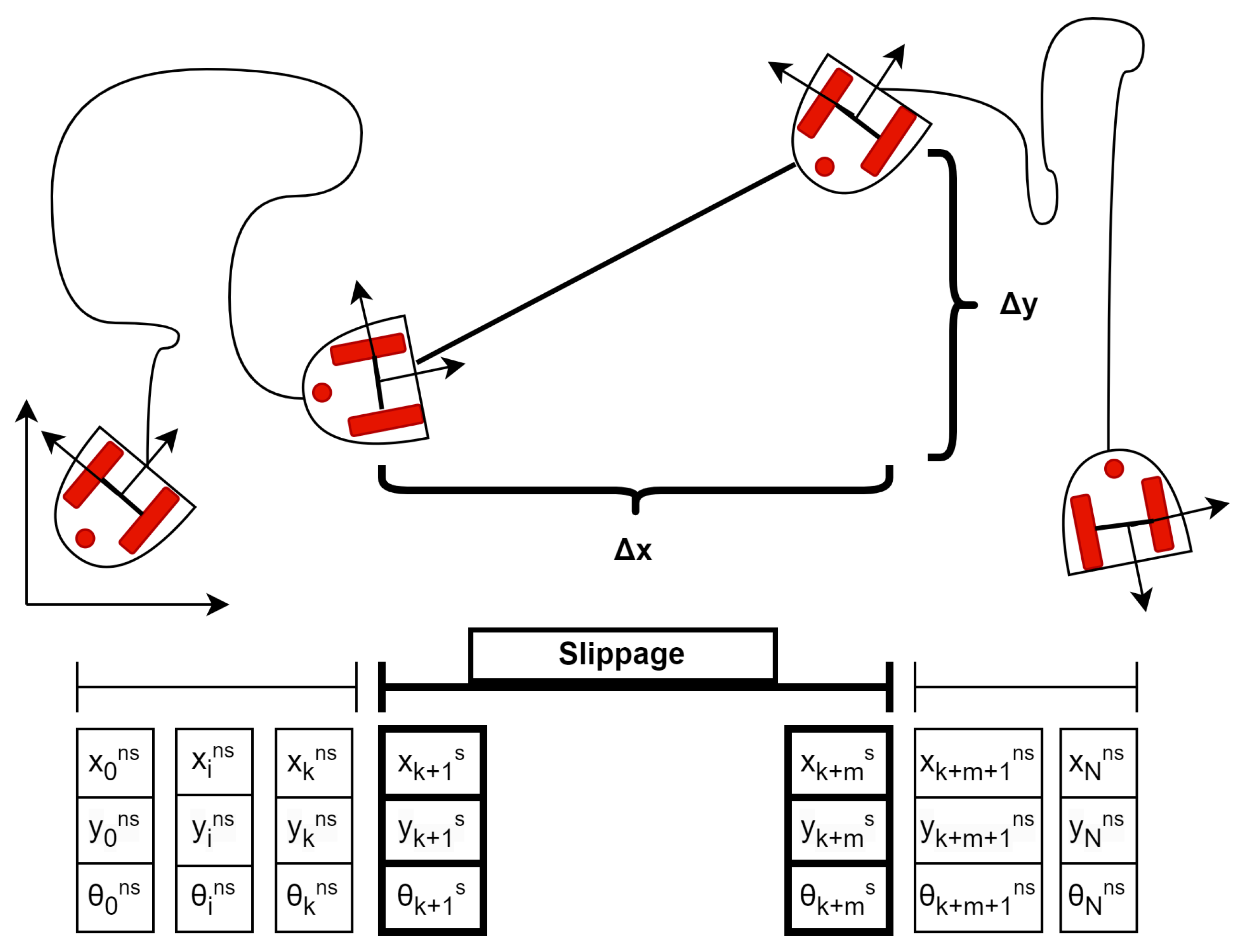
As for example, consider an arbitrary path where slippage phenomena occur during some steps (see
Figure 2). Without loss of generality, we assume that the slippage area, which is part of the main path, has a length of
m steps, with
where
N is the number of steps of the total path length (see A1). In the following, we use the superscript ‘
’ to indicate instances without slippage, and the superscript ‘
s’ to indicate segments consisting of multiple steps of time
where there happens some slippage in that area.
In order to exploit the methodology expressed in [
12] in the presence of slippage, Equation (
5) can be rewritten as follows:
where increments are defined as
and they can be computed either through ordinary odometry inference, whenever slippage is absent, or, in the presence of slippage, exploiting different other sensors (as described in the following of this Section).
3.1. Slippage Detection
Slippage can cause inconsistent measurements between the instantaneous displacement obtained from odometry and the actual displacement value. Slippage is primarily caused by lateral and longitudinal forces resulting from the vehicle’s motion, and low coefficient of friction. Though we can attempt to reduce these forces, slipping is inevitable when there is an unexpected change in the static coefficient of friction. There are several methodologies to detect slipping, such as comparing the kinematic model with pure rolling to another one that includes slipping.
Assuming to have access to an inertial measurement unit (IMU) mounted on board the vehicle, and assuming that the reference system of the IMU is aligned with the robot, an acceleration measurement
can be acquired from the system. In case of lateral slipping, the analysis of the acceleration
obtained from the IMU can reveal a non-zero value inconsistent with the differential model:
being
the rotation matrix for the coordinates’ transformation from the reference frame
to the body-fixed reference frame
obtained from angular velocity measurements, and
the gravity vector in
[
18].
On the other hand, the presence of frontal slipping, which may occur due to braking or acceleration, can be verified by checking the consistency between the differential model and the data from inertial accelerations: It could be verified whether there is consistency between the data of inertial acceleration in the presence of frontal slipping, which may occur due to braking or acceleration:
The violation of one of these conditions denotes the presence of slippage in the considered sub-track.
Remark 1. It should be noted that zero equality in the Equations (7) and (8) is only theoretical. From a practical point of view, a certain tolerance should be considered regarding the measurement error, namely:andwhere are suitable thresholds that can be set based on the IMU data sheet, combining the in-run bias stability and noise, as explained in detail in [21]. Such parameters are indeed a criterion for the selection of an IMU mostly adequate for the proposed algorithm (which is expected to last an amount of time of the order of a minute). Finally, to avoid false alarms caused by noise, violation of conditions (9) and (10) is checked for few steps instead of only one. 3.2. Slippage Estimation
Whenever a slippage condition is detected, the algorithm triggers an IMU-based motion reconstruction procedure to exploit the only correct data available and estimate the induced spatial displacements to further data correction. To this end, in this Section, we derive a procedure for the motion reconstruction based on IMU data only which has been recently developed in [
18,
19], and we briefly describe in the following. The inertial Unit provides the vehicle acceleration measurement
expressed in the body-fixed reference frame
, while, conversely, modern gyroscopes are able to provide absolute orientation with accuracy of the order of
degrees, allowing direct measurement of the angle
in
, and consequently to quickly identify the value of
. For sake of clarity, we assume that slipping occurs in a single area consisting of
m segments, namely:
We denote
and
resp. the orientation and forward velocity of the robot at the beginning of each slip segment. Since during slipping, there is no friction between the robot wheels and the ground, to reconstruct the motion in these
m segments, we adopt a uniformly accelerated model based on IMU data and we recur to the approach of [
18]:
being
the rotation matrix for the coordinates’ transformation from the body-fixed reference frame
to the reference frame
obtained from angular velocity measurements [
18],
the vehicle’s velocity in the body-fixed reference frame
obtained from encoders measurements,
the vehicle’s acceleration measurement in body reference frame
obtained from IMU, and
the gravity vector in
[
18].
Equations (11)–(13) together with Equation (17), allow for a proper exploitation of the heterogeneous data gathered from the sensors, together with the kinematics of the robot, to have an accurate estimation of robot localization through Equations (22) and (23) notwithstanding the possible presence of slippage.
Remark 2. Also, in this case, Equations (12) and (13) are computed using data , obtained through IMU acquisition. Combining Equations (12) and (13) with a sensor output model as Equation (1) of [21] allow also for easy computation of the maximum estimation error of , and starting from the IMU measurement of , . 3.3. Slippage-Compensated Odometric Parameters Estimation
Consider now the overall displacement, from time 0 to
along the path. Under the pure rolling condition, it is expressed by Equation (
A1) in
Appendix A. Taking into account the possible presence of slippage, Equation (
A1) can be reorganized introducing one term that encloses the possible presence of slippage:
It is worth noticing that the displacements
,
,
in Equations (14)–(16), do not depend on the unknown odometric parameters, but they can be considered known quantities under the assumptions of measurements from different sensors onboard. This allows us to adapt the original Least-Squares approach by keeping the information of all the non-corrupted sections, and by correcting the final position through the increments measured in the slippage sections only.
In order to exploit the above logic line, we introduce the following notation:
the following equations hold, which resemble the proposed no-slippage approach:
where the regressors
and
can be easily deduced from Equations (14)–(16).
The procedure is then repeated for multiple experiments collecting data from
P suitable trajectories, measurement data are stacked, and the new regressor is obtained (similarly to the original approach that led to Equations (
A6) and (A7)):
Finally, through a suitable number of random trajectories, it is possible to estimate the parameters
:
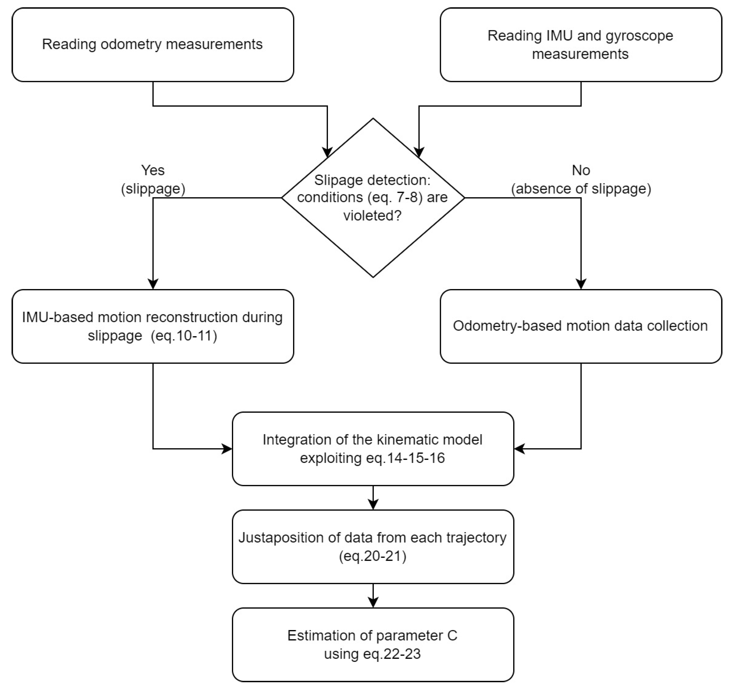
An overview of the whole calibration procedure described in this section is shown in the flowchart in
Figure 3.
Remark 3. If IMU data sheets are available, Equations (17), (22) and (23) can be equipped with the maximum error induced by the IMU measurements. Indeed, following the direction of Remark 2, setting where is computed using the measured values and is the estimation error (whose bound can be computed as suggested in Remark 2), using (23) it is possible to find the maximum estimation error of and caused by the IMU measurements. Similar considerations hold for and as well, making it possible, using (22), to find the maximum estimation error of and caused by the IMU measurements.
4. Numerical Simulations
The proposed methodology is validated through MATLAB simulations, providing important insights for the next experimental phase. Indeed, the final objective of this numerical simulation campaign is to assess the performance of the proposed approach in a controlled environment where the ground truth is exactly known.
We are interested in testing the online calibration method on ‘arbitrary’ paths that could be executed during standard operating activities of a mobile robot. To this aim, a two-dimensional grid including obstacles is considered, and a set of P free paths from an initial to a target position are simulated. We assume, without loss of generality, that the robot is equipped with a path planner to autonomously build these paths; the most common planners typically used in robotic applications are the rapidly exploring random tree (RRT) planner and the Probabilistic Road map (PRM) planner.
In order to test the proposed method, an arbitrary slippage is introduced by modifying the nominal absolute velocities of the robot proportionally to an arbitrary value
.
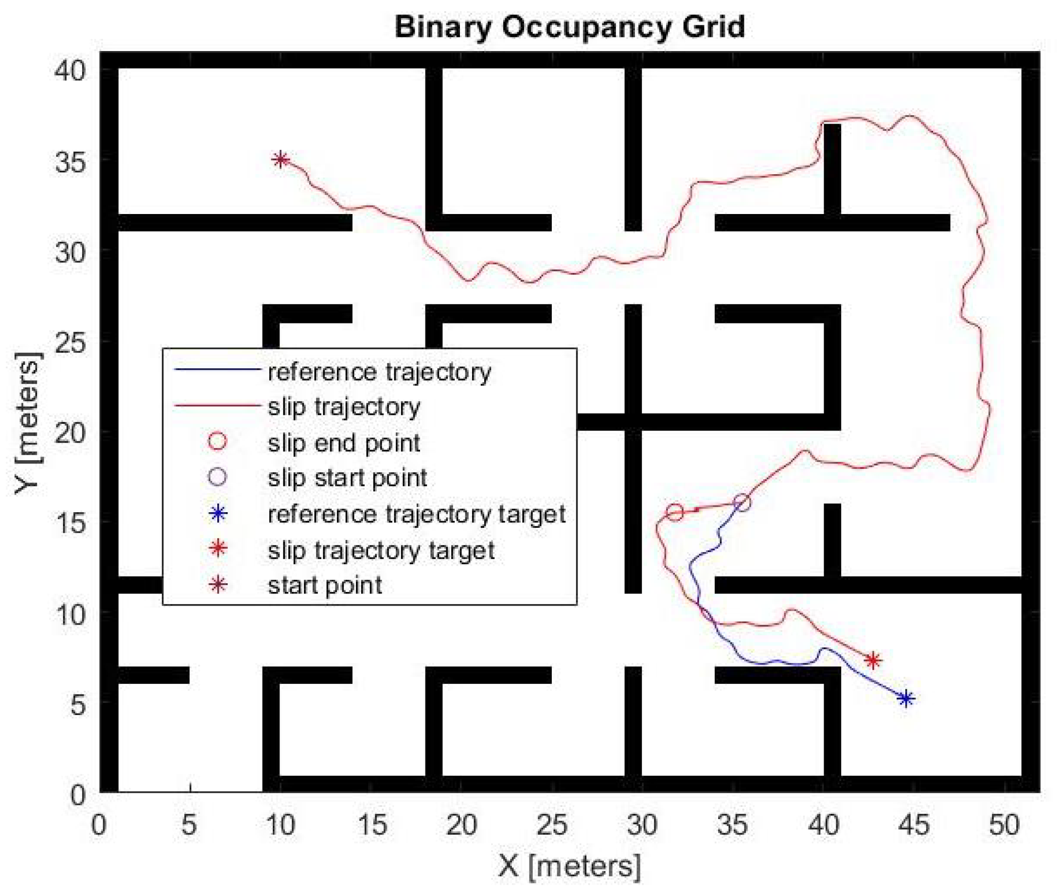
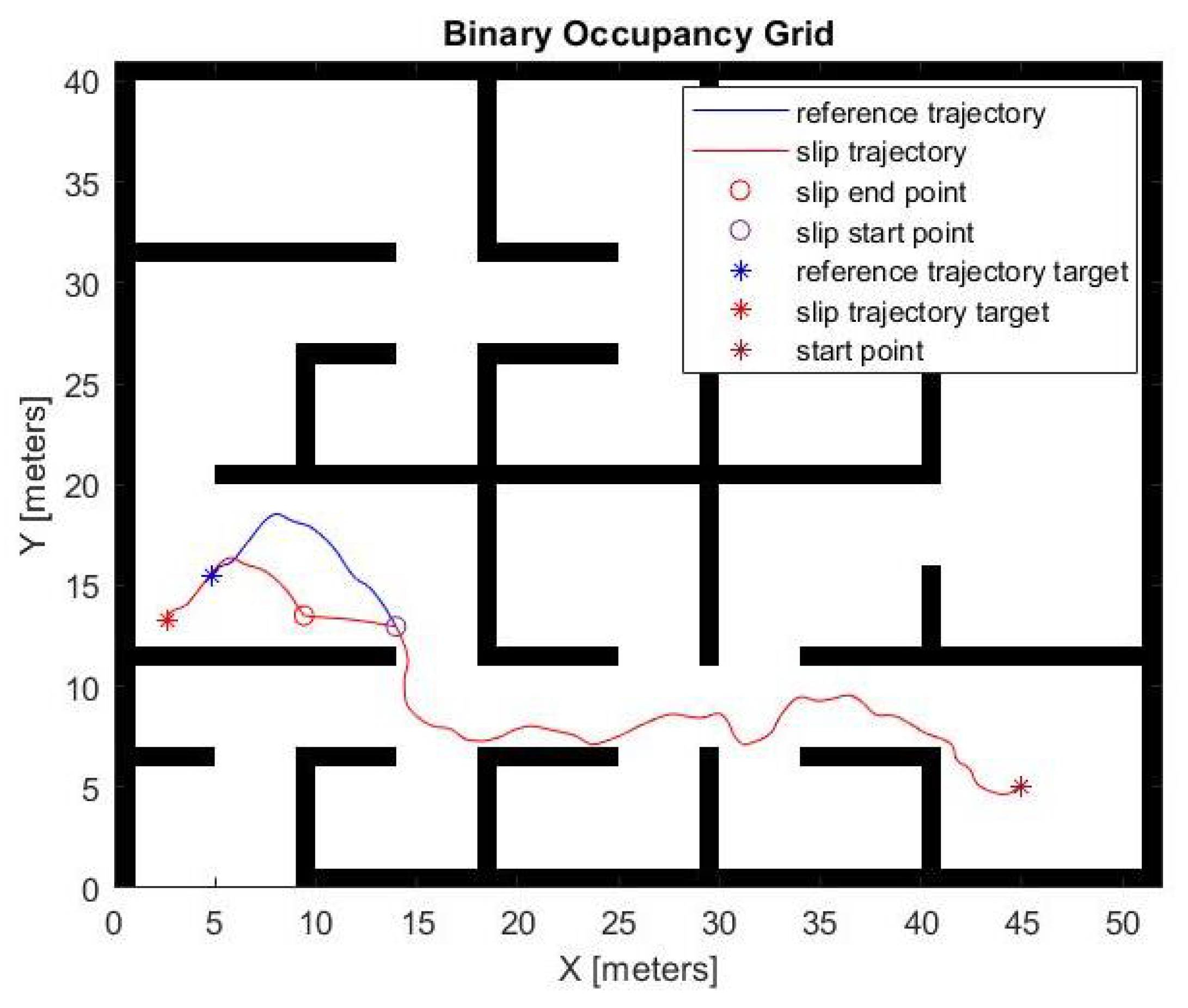
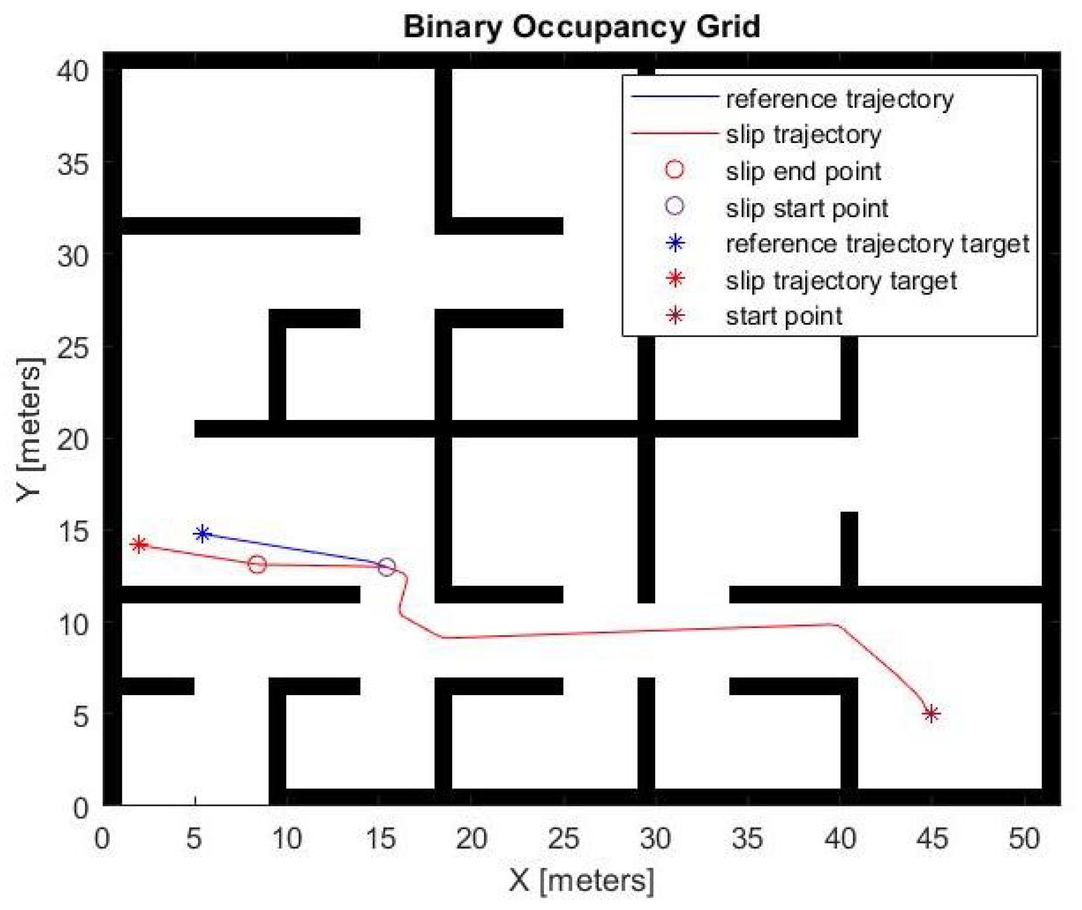
Figure 4 shows one example of the
P trajectories. The slip-free trajectory is depicted in blue, while the trajectory affected by the presence of slippage is depicted in red. In particular, the red path is obtained by arbitrarily modifying the nominal absolute velocities
(increased by a factor
) and
(reduced by a factor
). The resulting velocities generate frontal and lateral accelerations inconsistent with the odometric model as described in
Section 3.1. This allows a direct comparison between the ideal case in the absence of slippage (denoted by
‘ns’ in the following) and the two case studies where: (i) slippage is present but unidentified (denoted by
‘suc’), and (ii) slippage is present, properly estimated and managed with the proposed methodology (denoted by
‘sc’).
The presence of slippage is simulated for an interval , after that the robot proceeds in both simulated scenarios with the same nominal speed control signal, reaching two final target positions translated by a quantity , .
In order to ensure comparability of the trajectories, it is assumed that both trajectories reach their final target position and that the starting point and the two endpoints are not subject to any measurement error.
To perform a realistic test of the algorithm, nominal inputs and sensor measurements are perturbed by introducing a zero mean white Gaussian noise to the signals, as described in the following. The acquisition of the
signal is simulated with a signal-to-noise ratio of 30 dB. The estimation of the slippage
,
from IMU and gyro measurements is simulated with a signal-to-noise ratio of 30 dB. The acquisition of the wheels’ angular velocity
and
signals from encoders is simulated with a signal-to-noise ratio of 50 dB. The simulation is undertaken assuming a sampling period
[s] and the matrix
C containing the odometric parameters is equal to:
In the three scenarios (ideal ‘ns’, presence of slippage but unidentified ‘suc’, and presence of slippage properly estimated and managed ‘sc’), we compare the results obtained in the presence of noise measurements, or in its absence, considering the two different planners commonly used in robotic applications, i.e., the PRM planner and the RRT-Dubins planner (namely, the RRT planner where each path is made of Dubins curves with maximum turning radius equal to m).
Table 1 shows the estimations of the odometric parameters
and the corresponding estimation error
obtained in the absence of measurement noise considering
trajectories generated by the RRT-Dubins planner.
As expected, in the presence of slippage, proper detection of slippage occurrences and proper management of the measurements acquired during such steps using the proposed method allows for estimating the odometric parameters with higher precision than the conventional approach that does not take into account (by construction) any possible occurrence of slippage.
The effectiveness of the proposed methodology is also clear in the presence of noisy measurements.
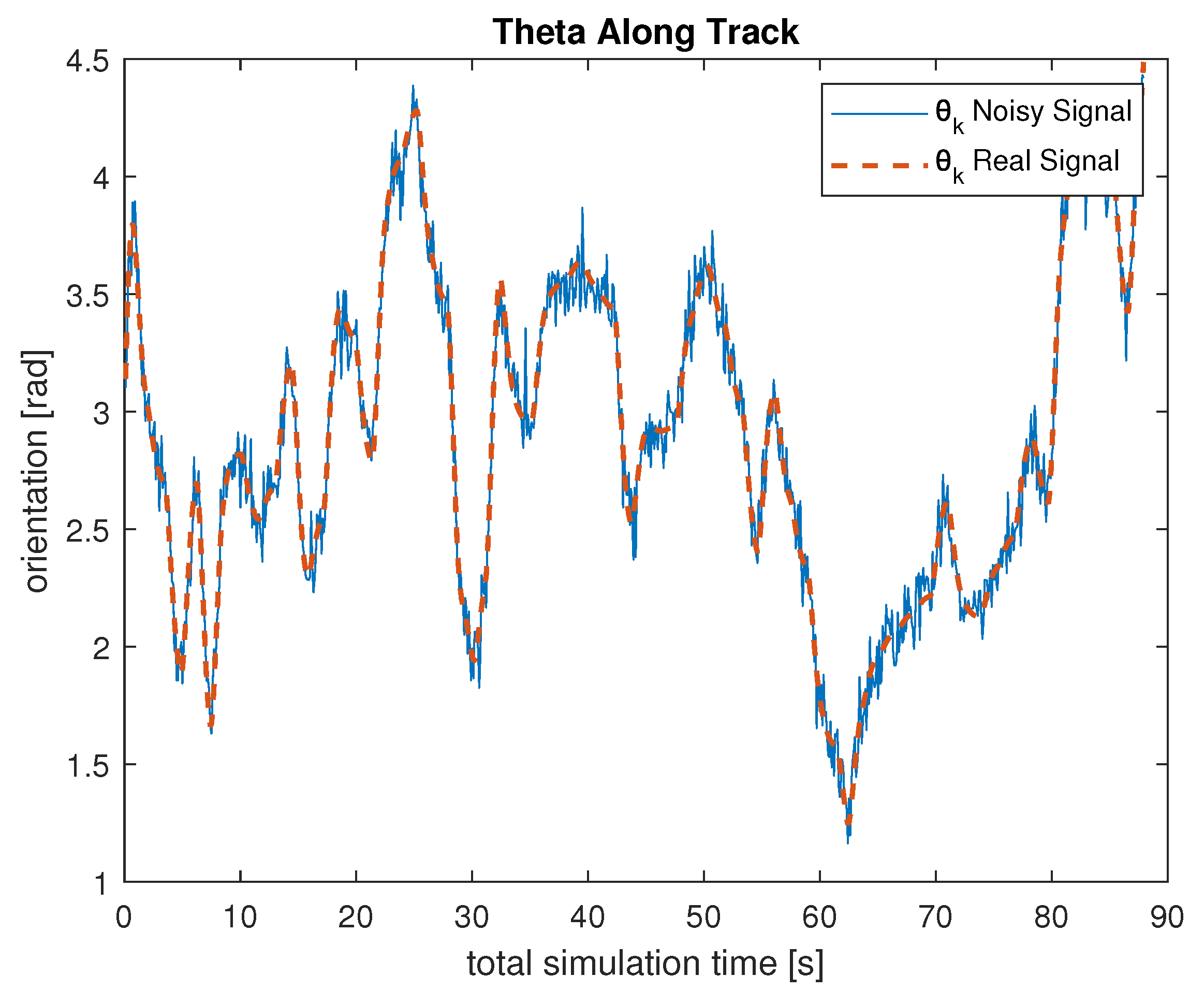
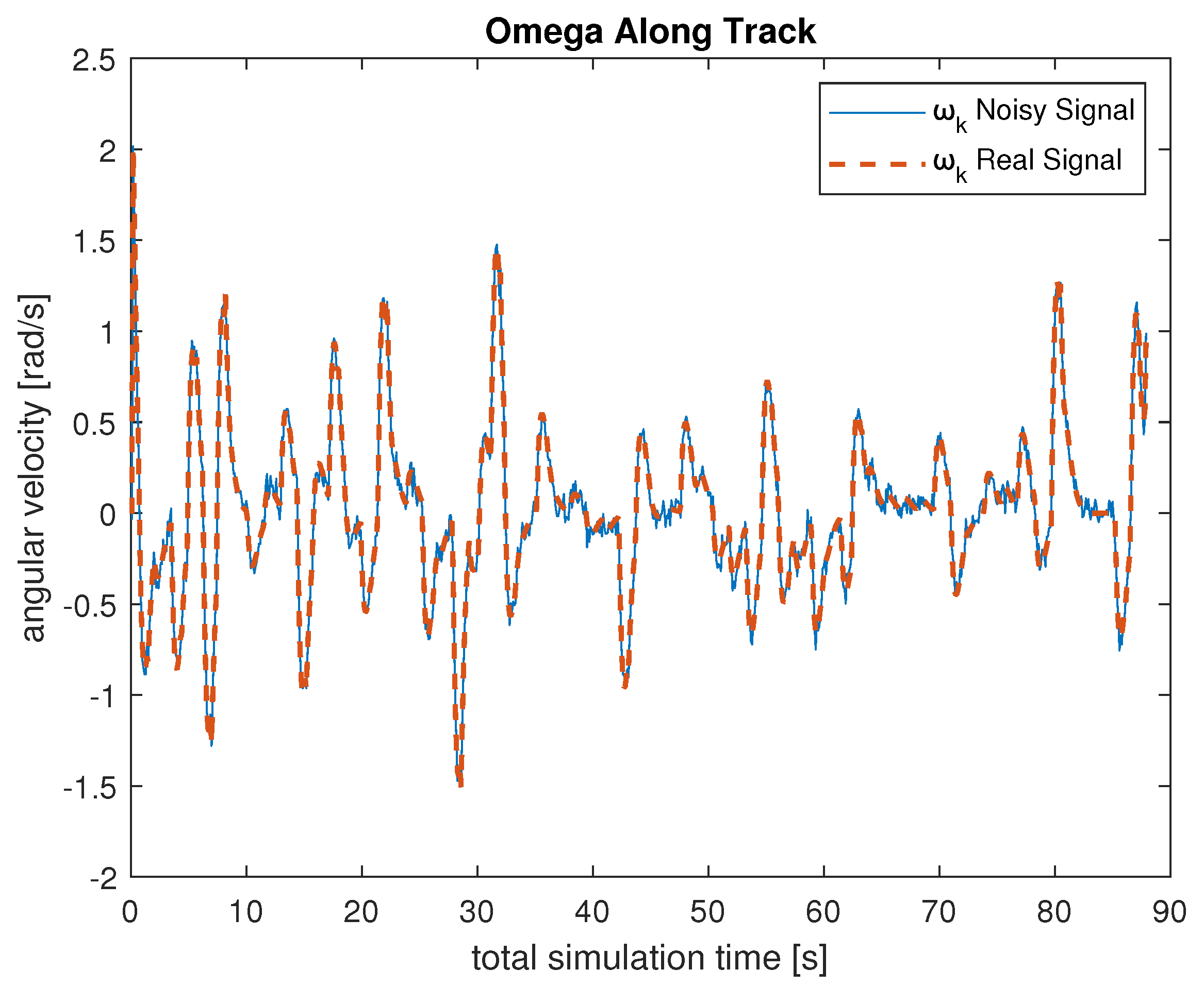
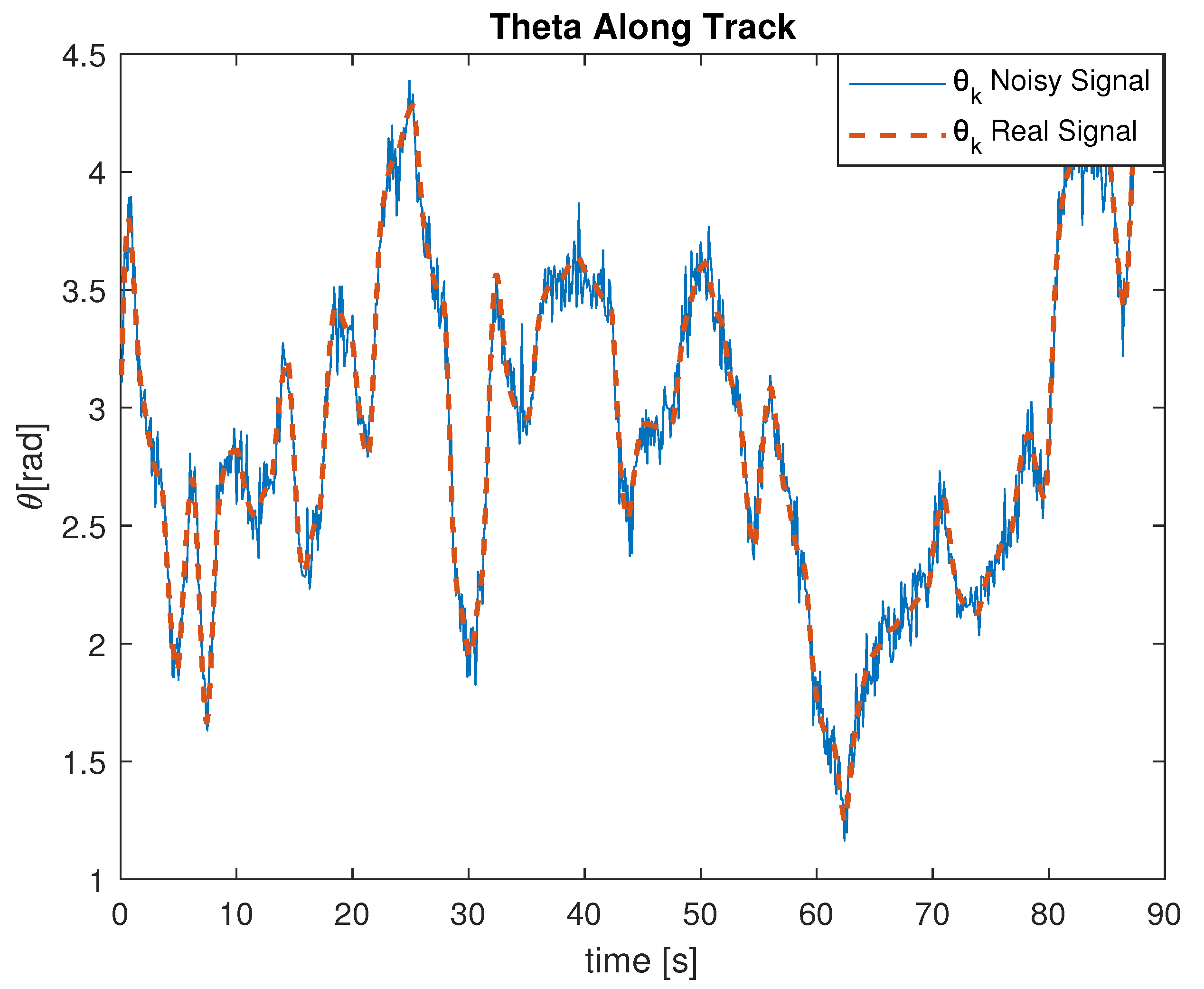
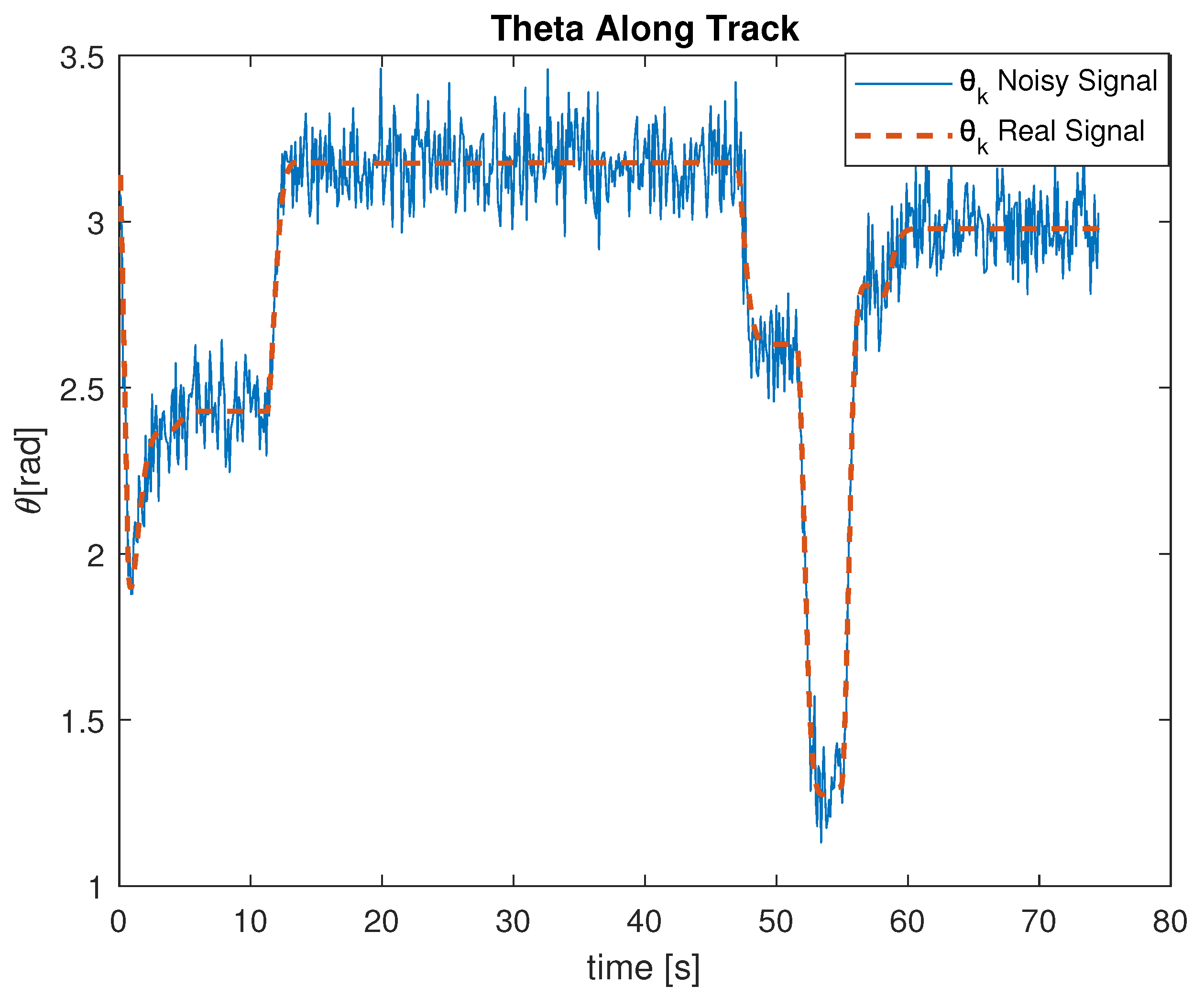
Figure 5 and
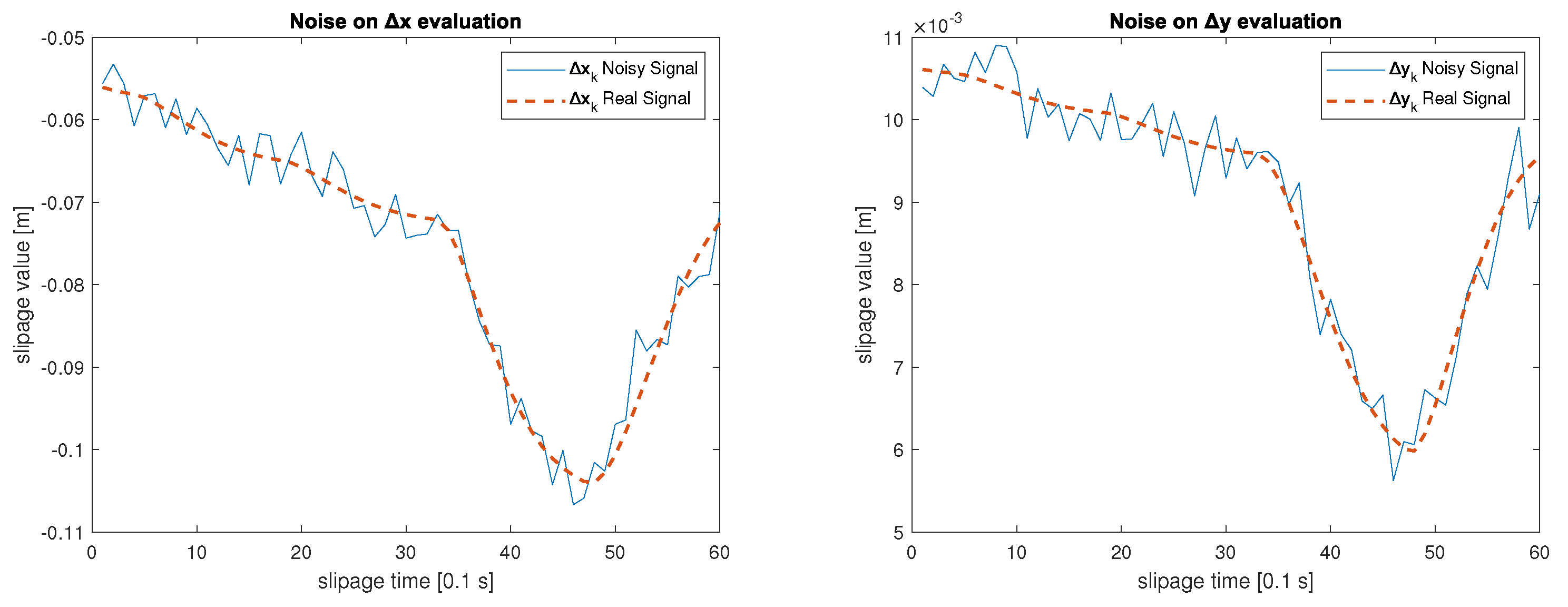
Figure 6 report an example of the noisy angular measurements acquired during a simulated trajectory, and
Figure 7 displays the relative displacements.
Table 2 shows the estimated values of the odometric parameters
and the corresponding estimation error
, obtained in the presence of measurement noise considering
trajectories generated by the RRT-Dubins planner in the three different scenarios: ideal with noisy measurements (denoted as
‘ns-noisy’), presence of slippage but unidentified with noisy measurements (denoted as
‘suc-noisy’), and the presence of slippage properly estimated and managed with noisy measurements (
‘sc-noisy’).
Table 3 and
Table 4 show the results of analogous simulations (both in the absence and presence of measurement noise for the different scenarios), when a PRM planner is adopted.
Figure 8 and
Figure 9 report an example of possible trajectories, both in the presence and absence of slippage, generated by the RRT-Dubins motion planner and the corresponding vehicle’s orientation during the motion. Next,
Figure 10 and
Figure 11 report an example of possible trajectories, in the presence and absence of slippage, generated by the PRM motion planner and the corresponding vehicle’s orientation during the motion.
Analyzing the results obtained in the different scenarios with the two motion planners, we can infer that if the number of analyzed paths increases, the use of different motion planners has a reduced impact on the estimation. However, when paths are characterized by significant variations in the orientation , a little improvement in estimation can be observed. The results of these trials show how the use of curved trajectories, such as those generated by the RRT-Dubins motion planner, allows for slightly better calibration results. For this reason, in the following, we proceeded with the simulation campaign considering only the RRT-Dubins motion planner.
To conclude the analysis, we investigated the impact of the methodology in the presence of slippage for an interval
of varying entities. In particular, in order to assess the resilience of the two methodologies in the absence and presence of slippage and noise measurement, we estimated the matrix
C assuming different values for
and 4 s. The results are reported in
Table 5. Analyzing the proposed methodology as
varies, it is observed that an increase in the slip time has the effect of a deterioration of the estimation. Nevertheless, even in the presence of considerable slippage and noisy signals, the proposed methodology allows obtaining an estimation of matrix
close to the real one, and thus performances similar to the estimation in the scenario without slipping
.
As a final remark, it is worth highlighting that exhaustive numerical experiments revealed a significant detrimental effect on the calibration accuracy when the measurement noise on the orientation , which is related to the gyroscope signals, increases, and the same holds considering the slippage , , which is related to the measurements obtained through both gyroscope and IMU. On the other hand, the impact is minimal when the measurement noise increases on a single wheel velocity.
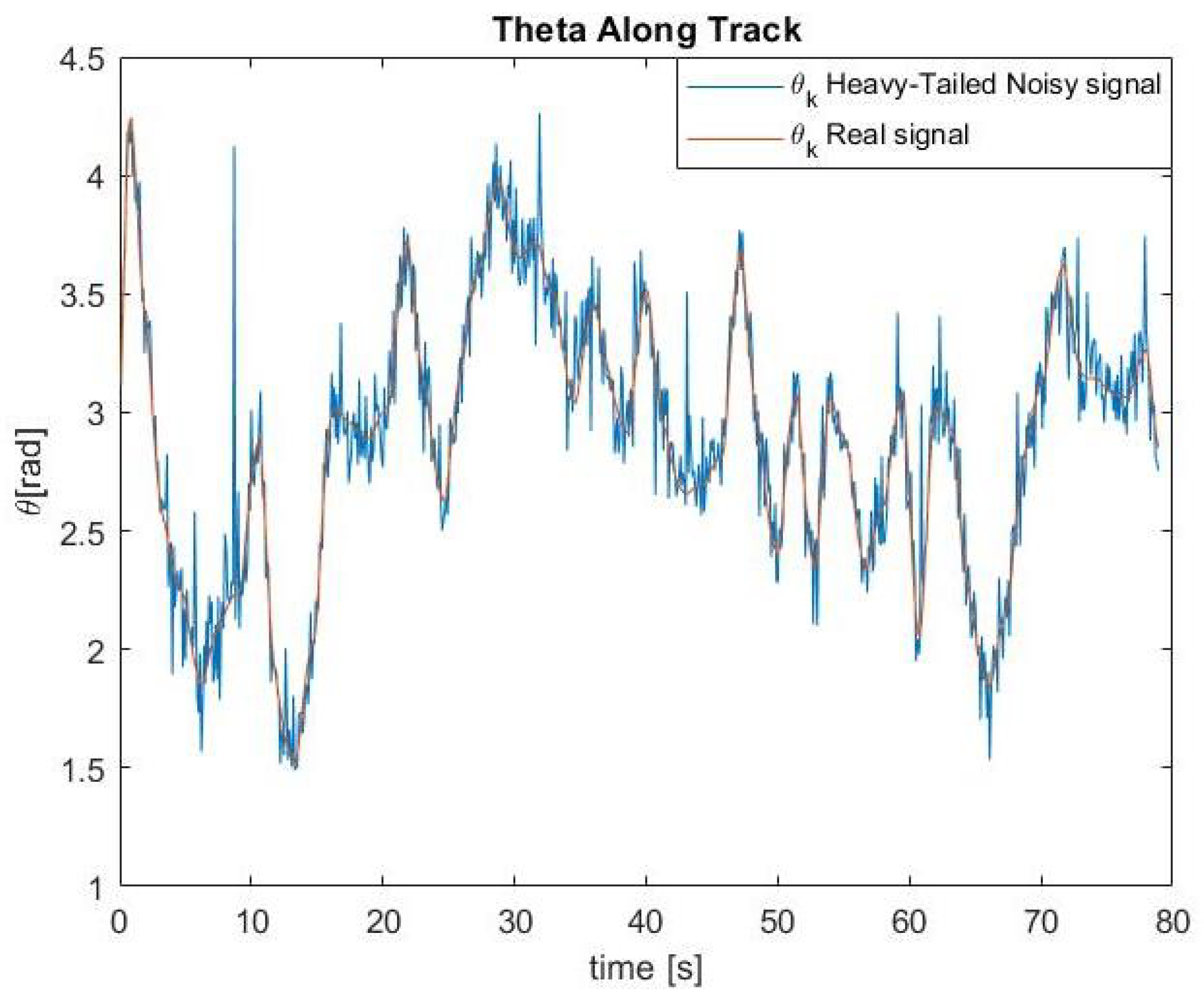
To evaluate the algorithm’s robustness in challenging conditions, including uneven terrain, electrical noise, and the presence of bumps or irregularities, we conducted tests involving the introduction of non-Gaussian noise to the Inertial Measurement Unit (IMU) signal. The ‘Heavy-tailed’ type noise was applied to the IMU using the Matlab command ‘makedist’ with parameters (‘LocationScale’, mu = 0, sigma = 1, nu = 3) and a noise amplitude of 0.1. as showed in
Figure 12 Additionally, we performed tests by introducing ‘Unknown But Bounded’ noise to the IMU signal. In this assessment, the Matlab function ‘rand’ with a maximum percentage amplitude of 0.1 was utilized to introduce the specified noise type. These evaluations, conducted over a sliding time of
= 6 on the 12 paths previously examined, demonstrated the algorithm’s sustained effectiveness, even in the presence of random peaks, as outlined in the following
Table 6.
Validation
Once we estimate the odometric parameters
, it becomes possible to assess the impact of each estimation on the robot localization’s performance. Hence, a numerical validation is undertaken to evaluate the calibration accuracy. The simulation is based on a set of 12 arbitrary paths generated by applying a sequence of control signals (
) to the vehicle, ensuring a condition free from slippage and noise. After averaging the previously estimated odometric parameters
, the velocity commands are converted into specific
and
values for each case. Finally, exploiting the kinematic model in Equation (
A1), the motion of the vehicle is characterized by the real matrix
C in Equation (24).
In order to quantify the impact of the estimation on an arbitrary path, the specific path computed through the actual C in Equation (24) is employed as reference nominal path. The behavior of the robots, starting from a prescribed initial position and moving according to the wheel velocity control signals induced by the different estimation , is evaluated using the following metrics:
- -
the average distance error over paths
,
- -
the average final distance error
,
- -
the average orientation error over the paths
,
- -
and the average final orientation error
,
being
n the total number of samples over the paths. The results obtained are presented in
Table 7.
The simulation results reveal that as the estimation of matrix C deteriorates, positioning errors progressively increase with higher
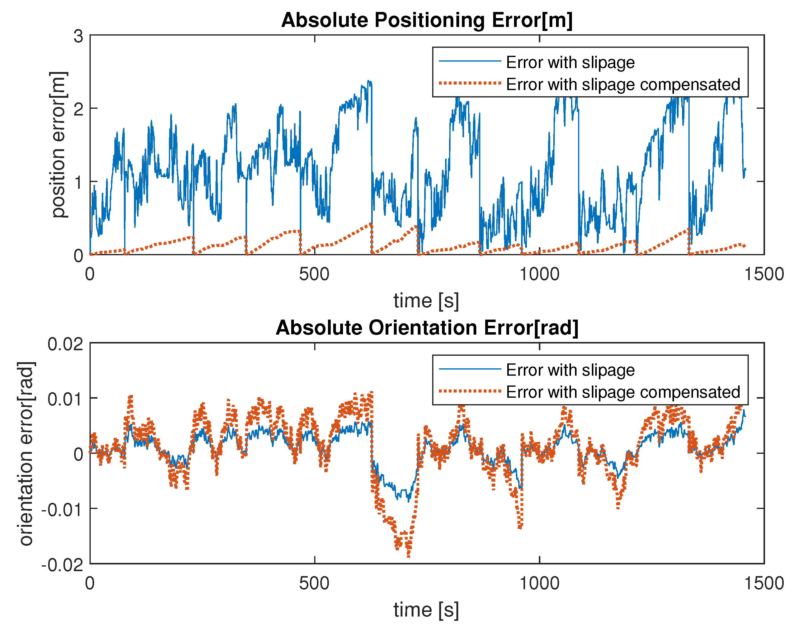
values, ultimately causing positioning errors exceeding one meter when uncompensated slipping occurs. However, numerical experiments also demonstrate that the proposed methodology greatly reduces both positioning and orientation errors, even in the case of noisy sensors. The effect of the proposed methodology is also highlighted in
Figure 13, where it is possible to compare the positioning and orientation errors, over 12 trajectories, between the
scenario and the
scenario. While there is a slight increase in orientation error, a substantial reduction in positioning error is observed, reaching a decrease of an order of magnitude as presented in
Table 8. This confirms the effectiveness of the proposed approach when slippage phenomena occur during the online calibration procedure.

