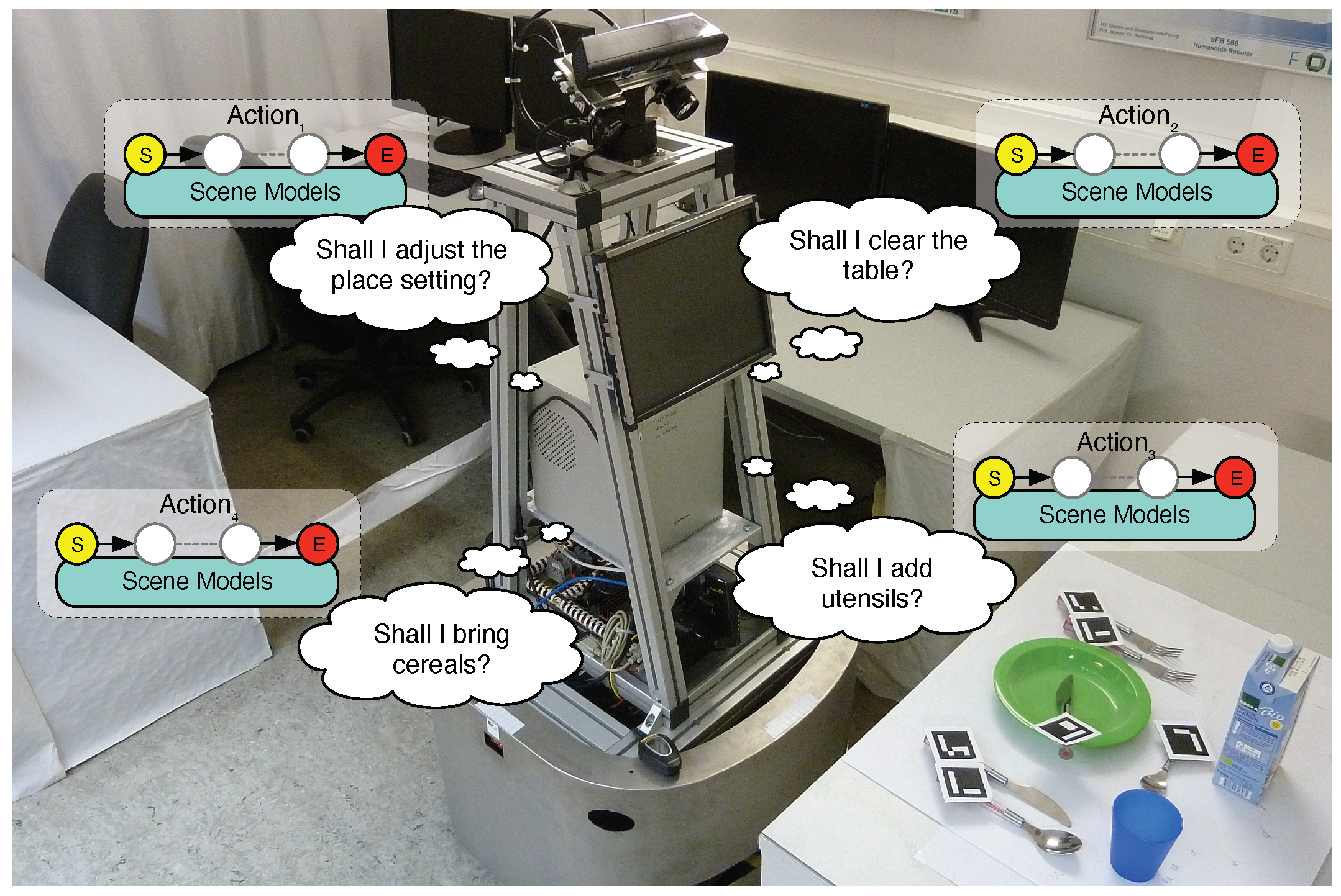
Figure 1.
Motivating example for scene recognition: Our mobile robot MILD looking at an object configuration (a.k.a. an arrangement). It reasons which of its actions to apply.
Figure 1.
Motivating example for scene recognition: Our mobile robot MILD looking at an object configuration (a.k.a. an arrangement). It reasons which of its actions to apply.
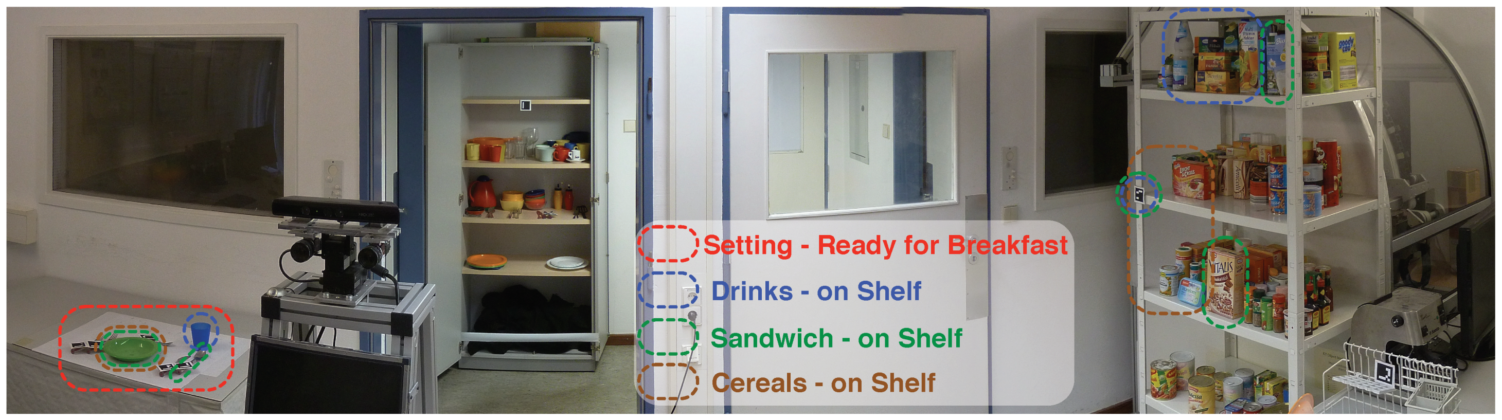
Figure 2.
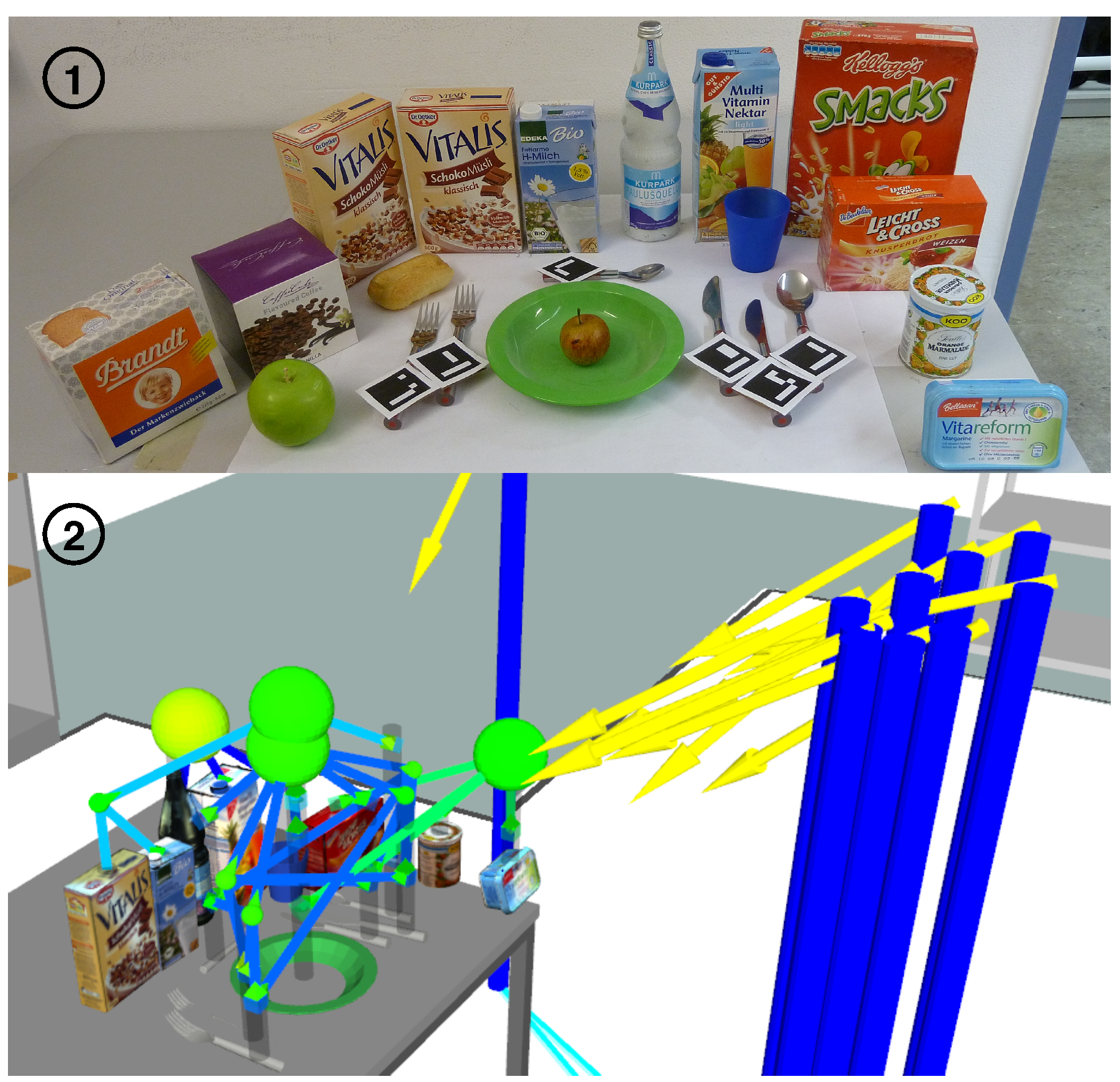
Experimental setup mimicking a kitchen. The objects are distributed over a table, a cupboard, and some shelves. Colored dashed boxes are used to discern the searched objects from the clutter and to assign objects to exemplary scene categories.
Figure 2.
Experimental setup mimicking a kitchen. The objects are distributed over a table, a cupboard, and some shelves. Colored dashed boxes are used to discern the searched objects from the clutter and to assign objects to exemplary scene categories.
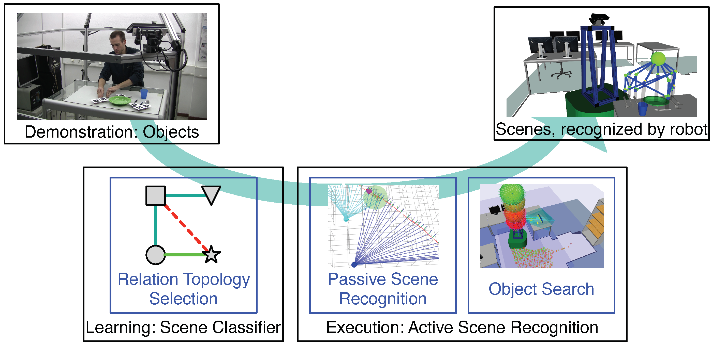
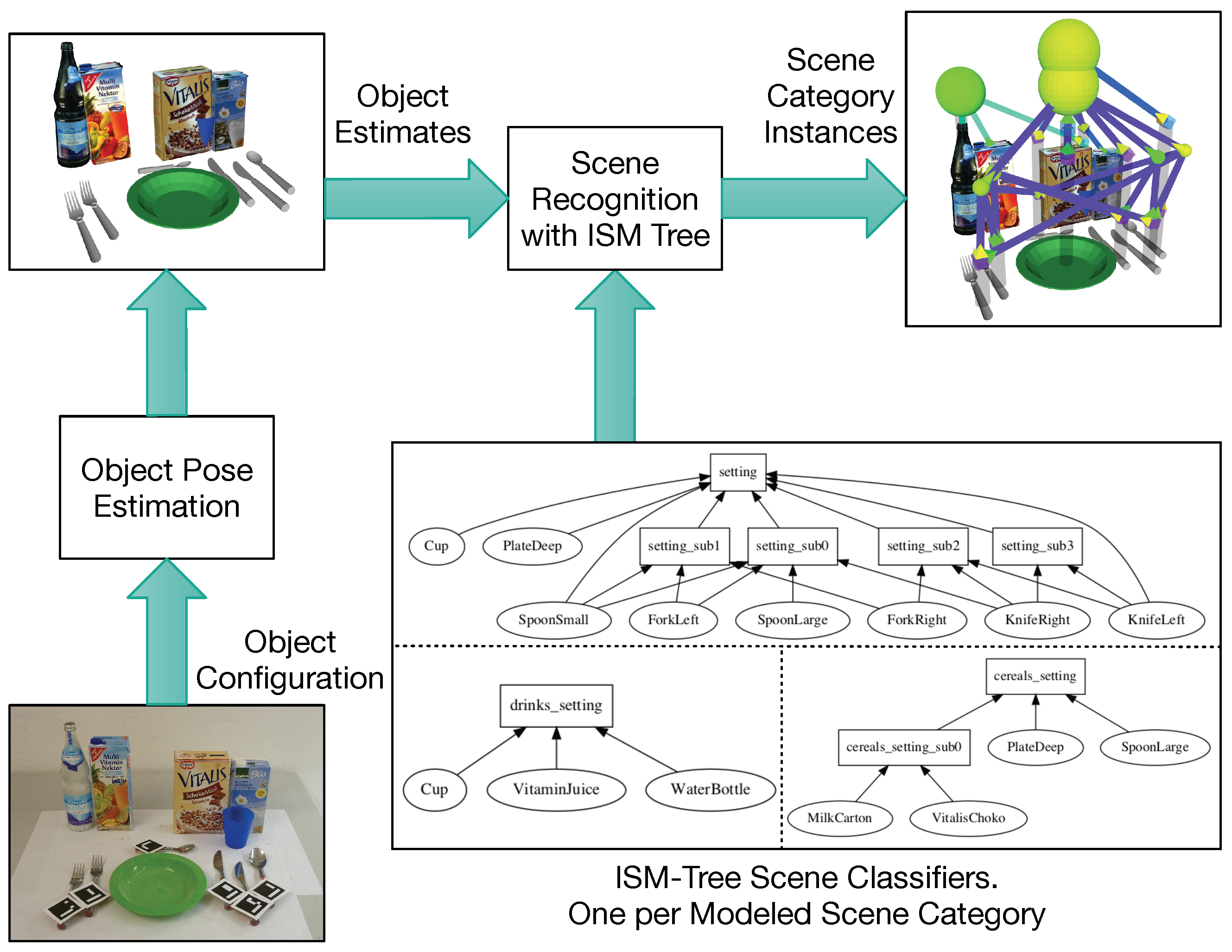
Figure 3.
Overview of the research problems (in blue) addressed by our overall approach. At the top are the inputs and outputs of our approach. Below are the two phases of our approach: scene classifier learning and ASR execution.
Figure 3.
Overview of the research problems (in blue) addressed by our overall approach. At the top are the inputs and outputs of our approach. Below are the two phases of our approach: scene classifier learning and ASR execution.
Figure 4.
Overview of the inputs and outputs of passive scene recognition. Spheres represent increasing confidences of outputs by colors from red to green.
Figure 4.
Overview of the inputs and outputs of passive scene recognition. Spheres represent increasing confidences of outputs by colors from red to green.
Figure 5.
Image 1: Snapshot of a demonstration. Image 2: Demonstrated object trajectories as sequences of object estimates. The cup is always to the right of the plate, and both in front of the box. Image 3: Relative poses, visualized as arrows pointing to a reference, form the relations in our scene classifier. Here, the classifier models the relations “cup-box” and “plate-box”. Image 4: Objects voting on poses of the reference using the relations from image 3. Image 5: Accumulator filled with votes. Image 6: Here, the cup is to the left of the plate, which contradicts the demonstration. The learned ISM does not recognize this, as it does not model the “cup-plate” relation. It outputs a false positive.
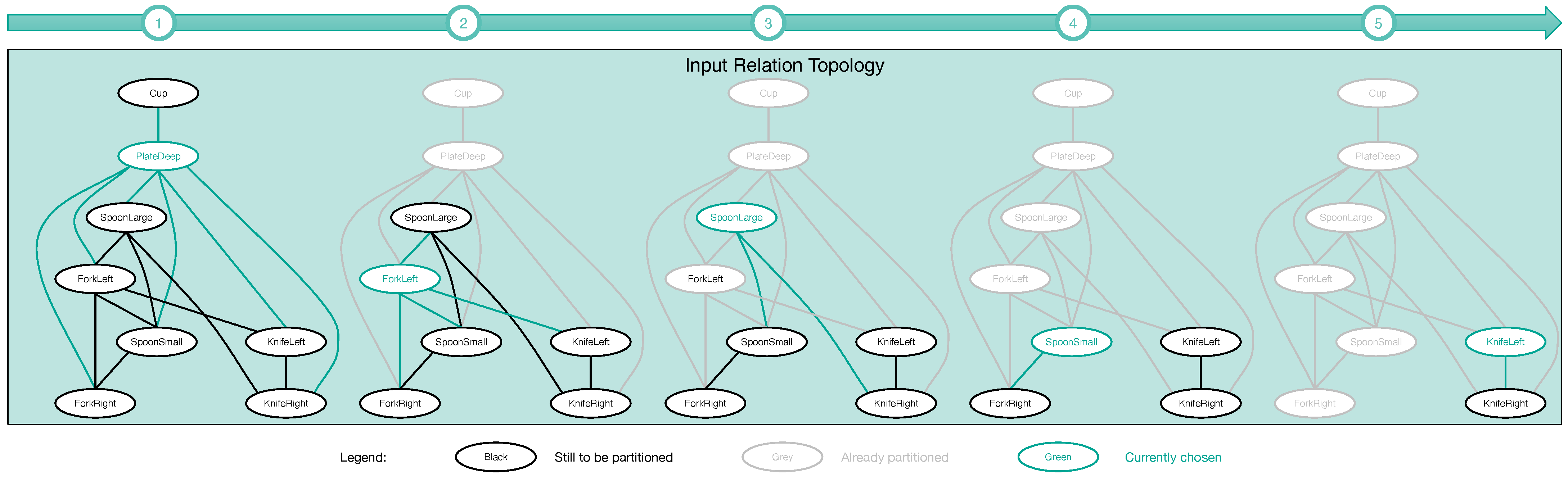
Figure 6.
Algorithm—how the connected relation topology from which we generated the ISM tree in
Figure 8—is first partitioned. The partitioning includes five iterations. It starts at the leftmost graph and ends at the rightmost. In each iteration, a portion of the connected topology, colored green, is converted into a separate star-shaped topology. All stars are on the left of
Figure 7.
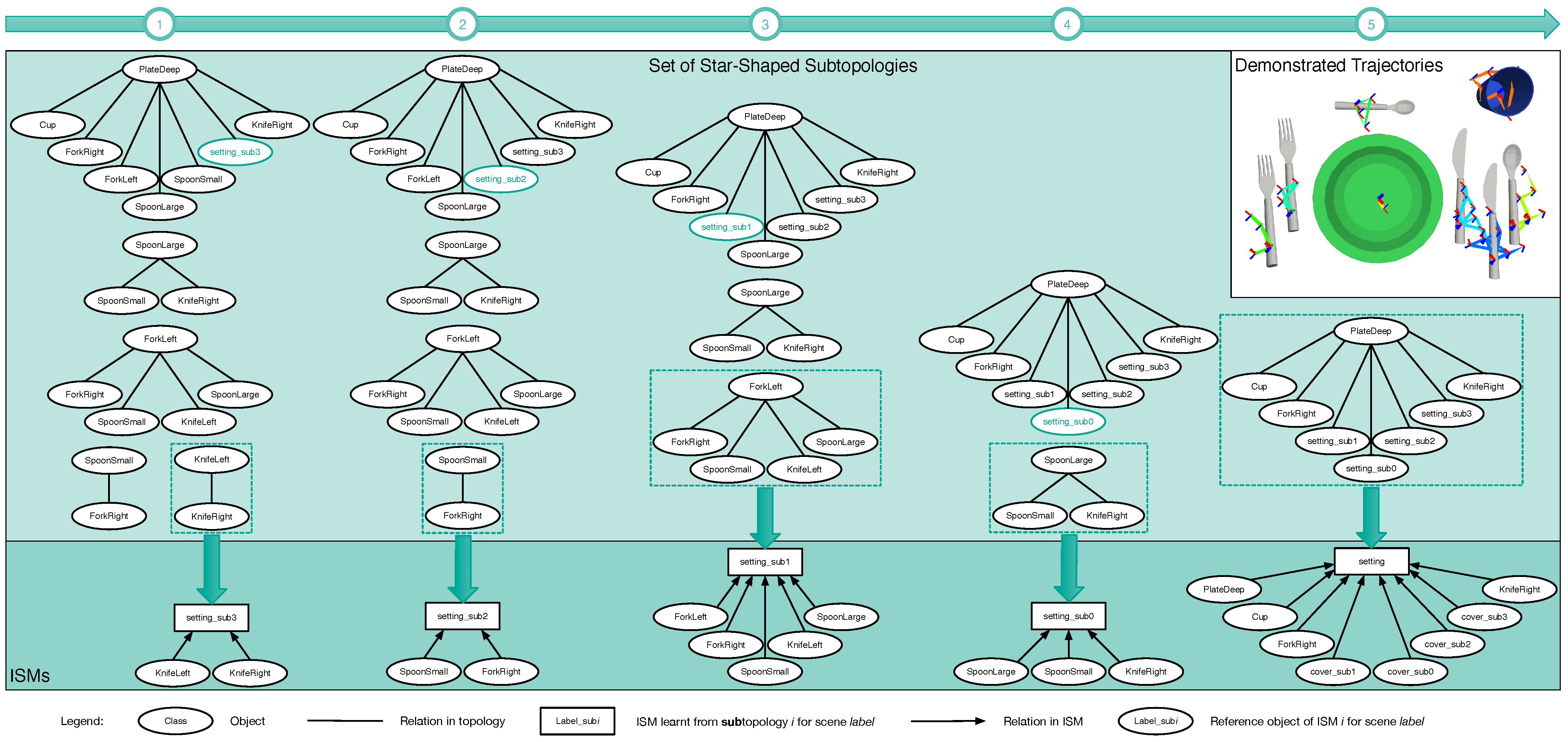
Figure 7.
Algorithm—how an ISM tree is generated from the star topologies—shown in the leftmost column (see 1). In each of the five depicted iterations, a star topology is selected to learn a single ISM using the object trajectories for scene category “Setting-Ready for Breakfast”. Dashed boxes show the selected stars, whereas arrows link these stars to the learned ISMs.
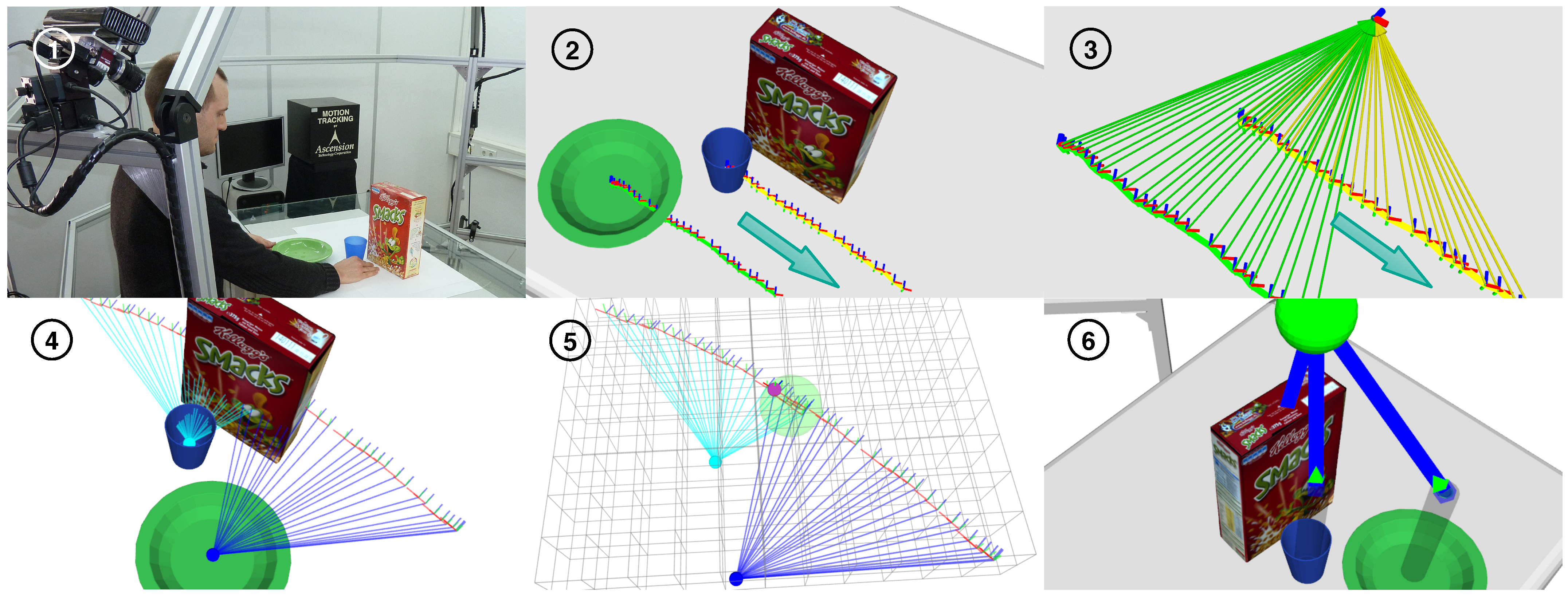
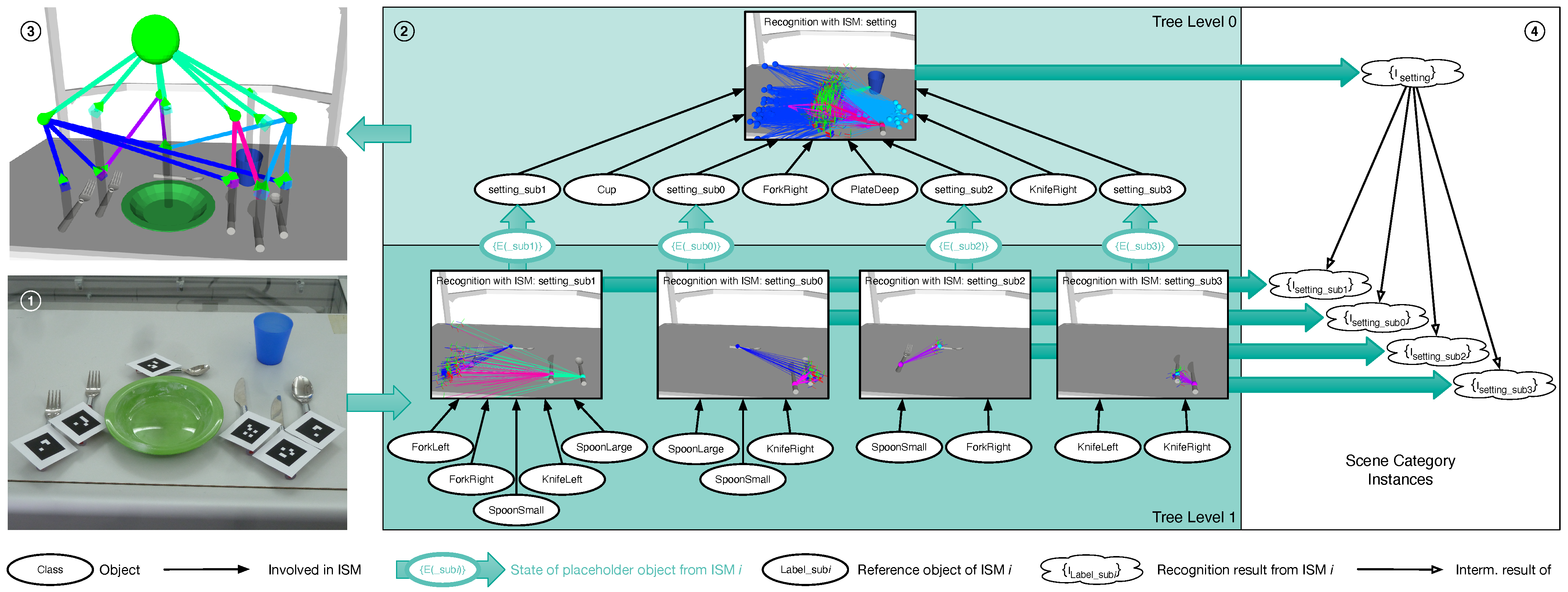
Figure 8.
Algorithm—how passive scene recognition works with an ISM tree. As soon as object poses estimated from the configuration in 1 are passed to the tree, data flows in 2 from the tree’s bottom to its top, eventually yielding the scene category instance shown in 3. This instance is made up of the recognition results in 4, which are returned by the single ISMs.
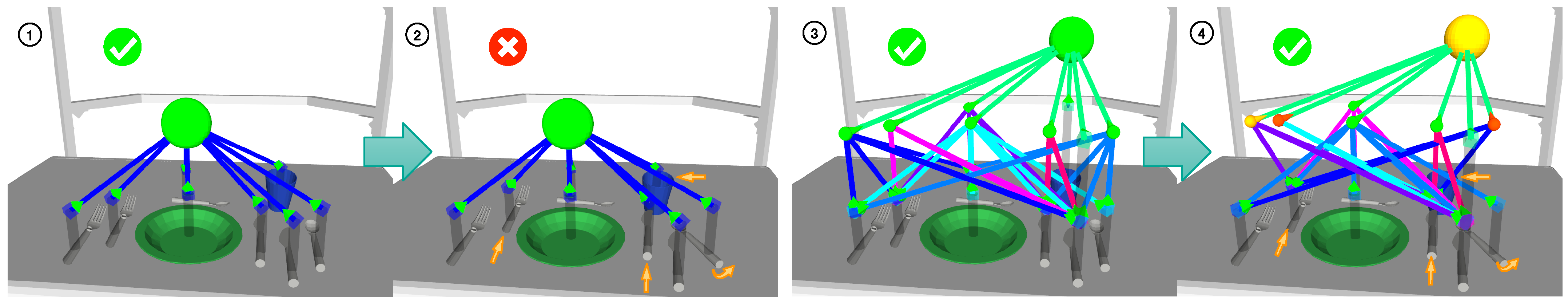
Figure 9.
Results from ISM trees for the same demonstration, but learned with different topologies. Valid results are annotated with a tick in green, invalid results by a cross in red. In images 1 and 2, a star is used. In images 3 and 4, a complete topology is used. In images 1 and 3, valid object configurations are processed. Instead, images 2 and 4 show invalid configurations.
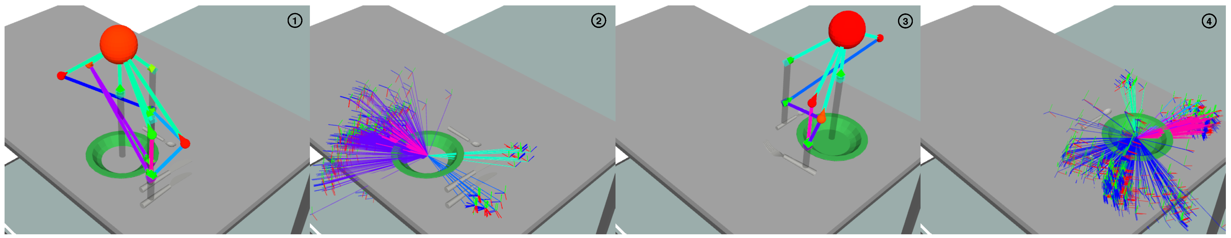
Figure 10.
Example of how scene recognition (see images 1 and 3) and object pose prediction (see images 2 and 4) can compensate for changing object poses. The results they return are equivalent, even though the localized objects are rotated by between images 1 and 2 and between images 3 and 4.
Figure 10.
Example of how scene recognition (see images 1 and 3) and object pose prediction (see images 2 and 4) can compensate for changing object poses. The results they return are equivalent, even though the localized objects are rotated by between images 1 and 2 and between images 3 and 4.
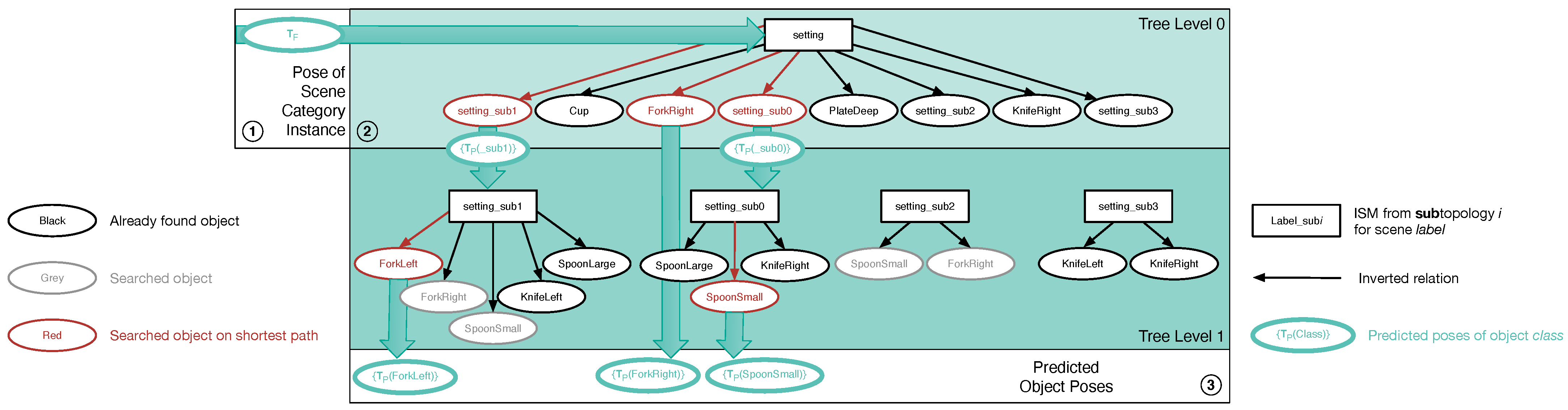
Figure 11.
Algorithm—how the poses of searched objects are predicted with an ISM tree. The incomplete scene category instance in 1 is input and causes data to flow through the tree in 2. Unlike scene recognition, data flows from the tree’s top to its bottom, while relative poses from different inverted spatial relations are combined. The resulting predictions are visible in 3.
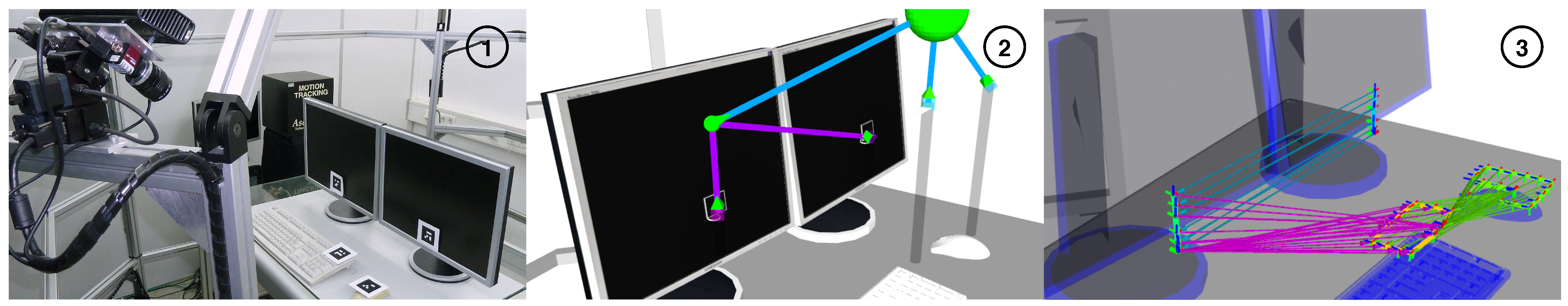
Figure 12.
Image 1: Snapshot of the demonstration for scene category “Office”. Image 3: The ISM tree for this category, including the relative poses in its relations and the demonstrated poses. Image 2: Result of applying this tree onto the configuration “Correct-configuration”.
Figure 12.
Image 1: Snapshot of the demonstration for scene category “Office”. Image 3: The ISM tree for this category, including the relative poses in its relations and the demonstrated poses. Image 2: Result of applying this tree onto the configuration “Correct-configuration”.
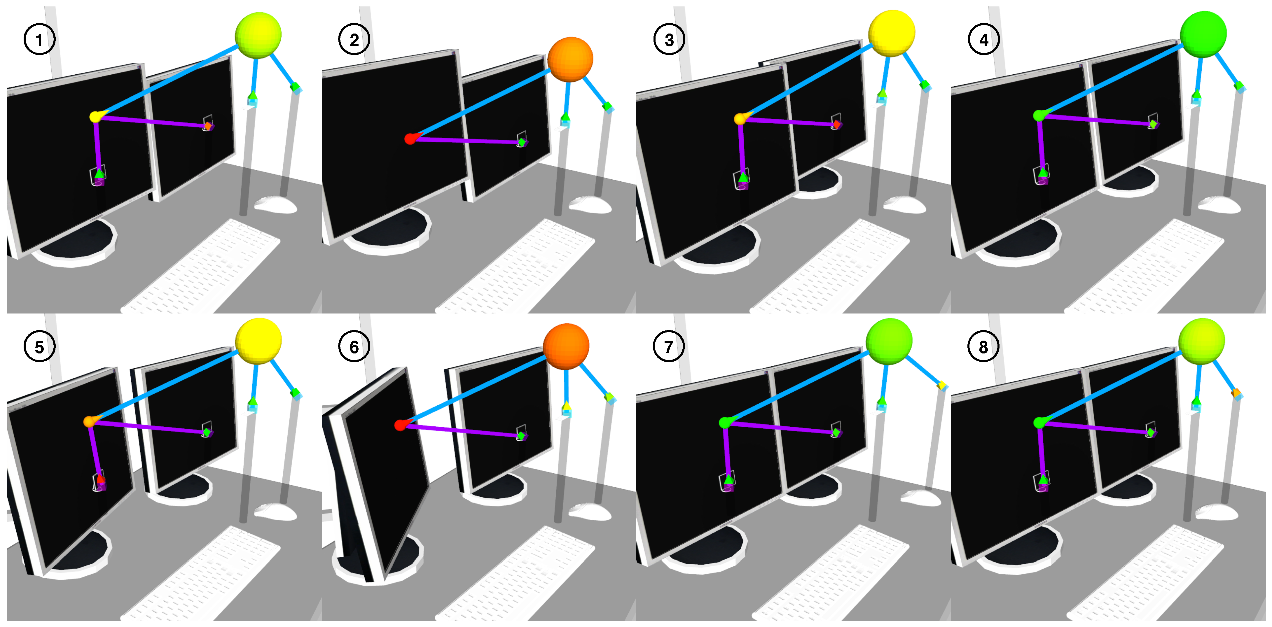
Figure 13.
Visualization of the scene category instances that an ISM tree for the category “Office” recognized in the physical object configurations “RightScreen-half-lowered” (image 1), “RightScreen-fully-lowered” (image 2), “LeftScreen-half-front” (image 3), “RightScreen-half-right” (image 4), “LeftScreen-half-rotated” (image 5), “LeftScreen-fully-rotated” (image 6), “Mouse-half-right” (image 7), and “Mouse-half-rotated” (image 8).
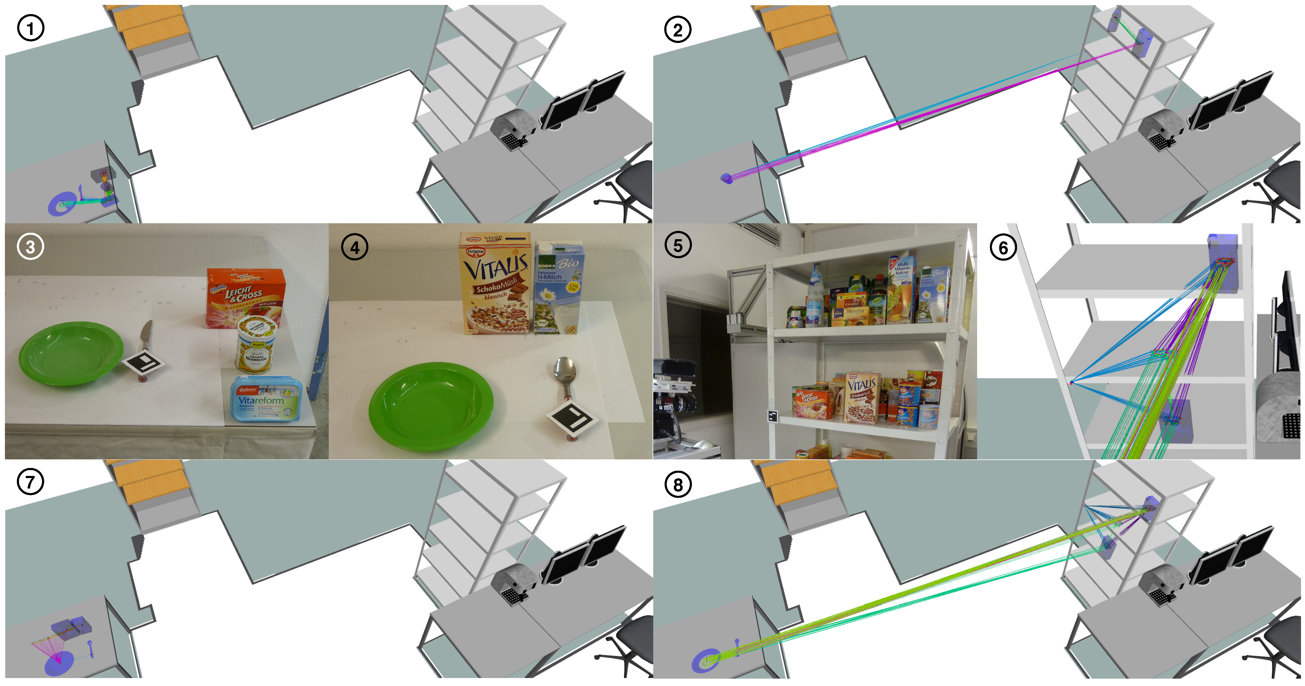
Figure 14.
Object trajectories demonstrated for the scene categories “Sandwich-Setting” (images 1, 3), “Drinks-on Shelf” (images 2, 5), “Cereals-Setting” (images 4, 7), and “Cereals-on Shelf” (images 6, 8) in our kitchen setup, as well as the spatial relations inside the ISM trees learned for these categories.
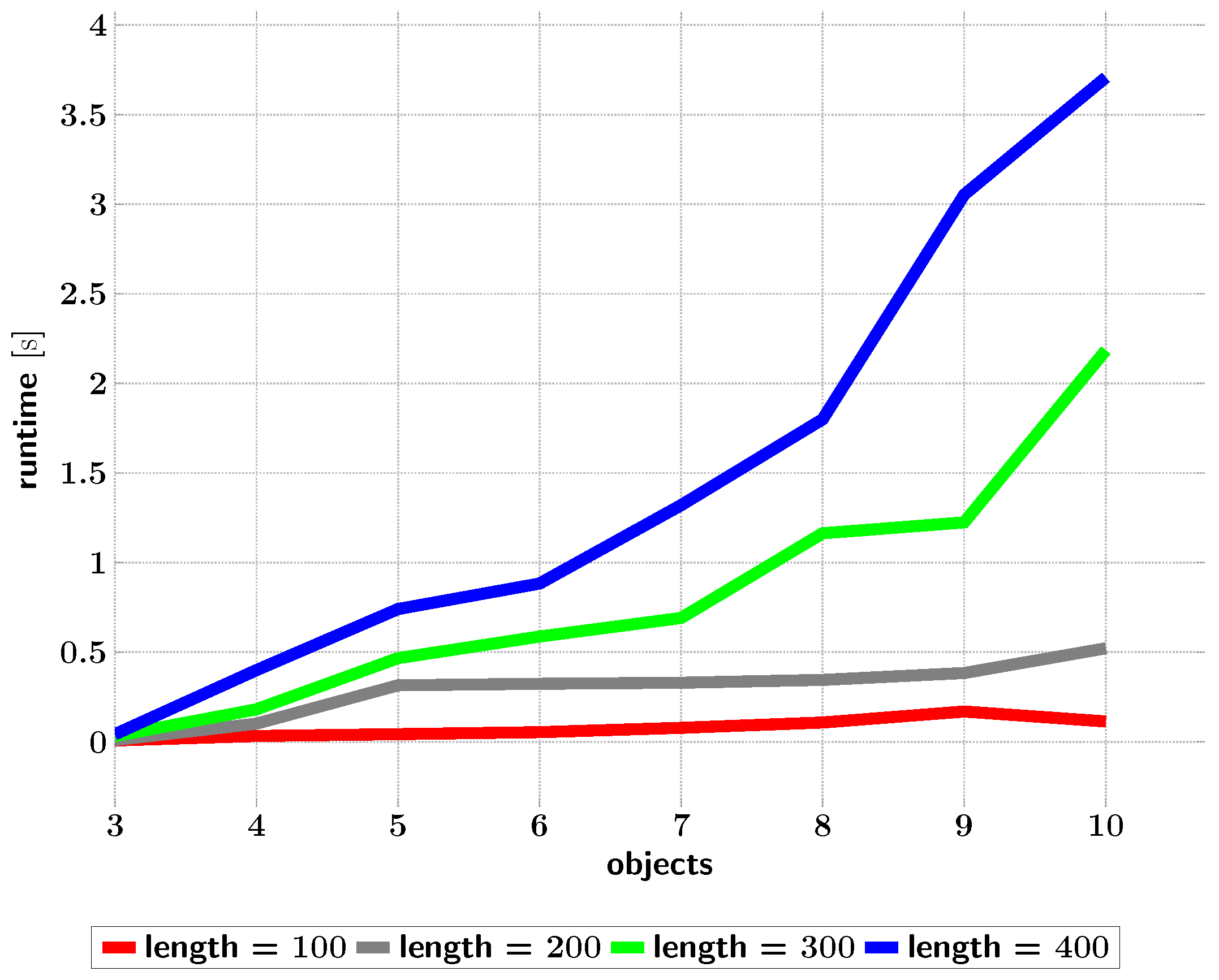
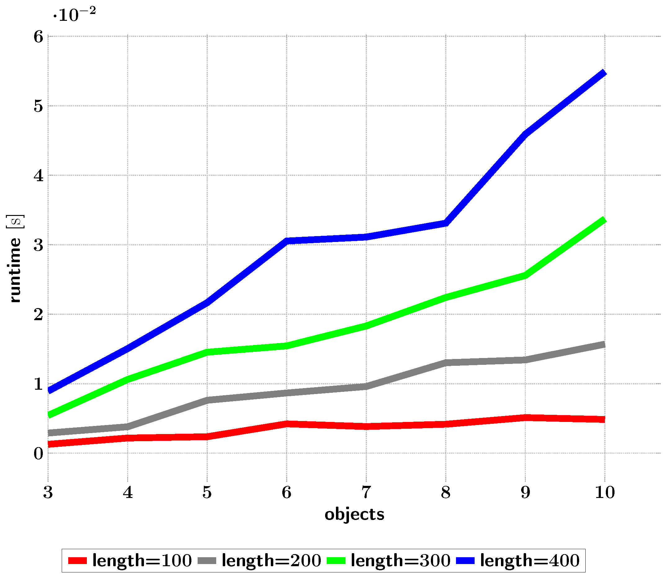
Figure 15.
Times taken for ISM trees (from optimized topologies) to recognize scenes depending on the trajectory lengths in their datasets.
Figure 15.
Times taken for ISM trees (from optimized topologies) to recognize scenes depending on the trajectory lengths in their datasets.
Figure 16.
Influence of object orientations on pose prediction: Images 1 and 2 show s1_e1 and s1_e2, respectively. Between s1_e1 and s1_e2, all objects on the shelves (right) were rotated. Images 1 and 2: Recognized scenes and camera views MILD adopted. Image 3: Snapshot during the execution of s1_e2. The miniature objects correspond to predicted poses.
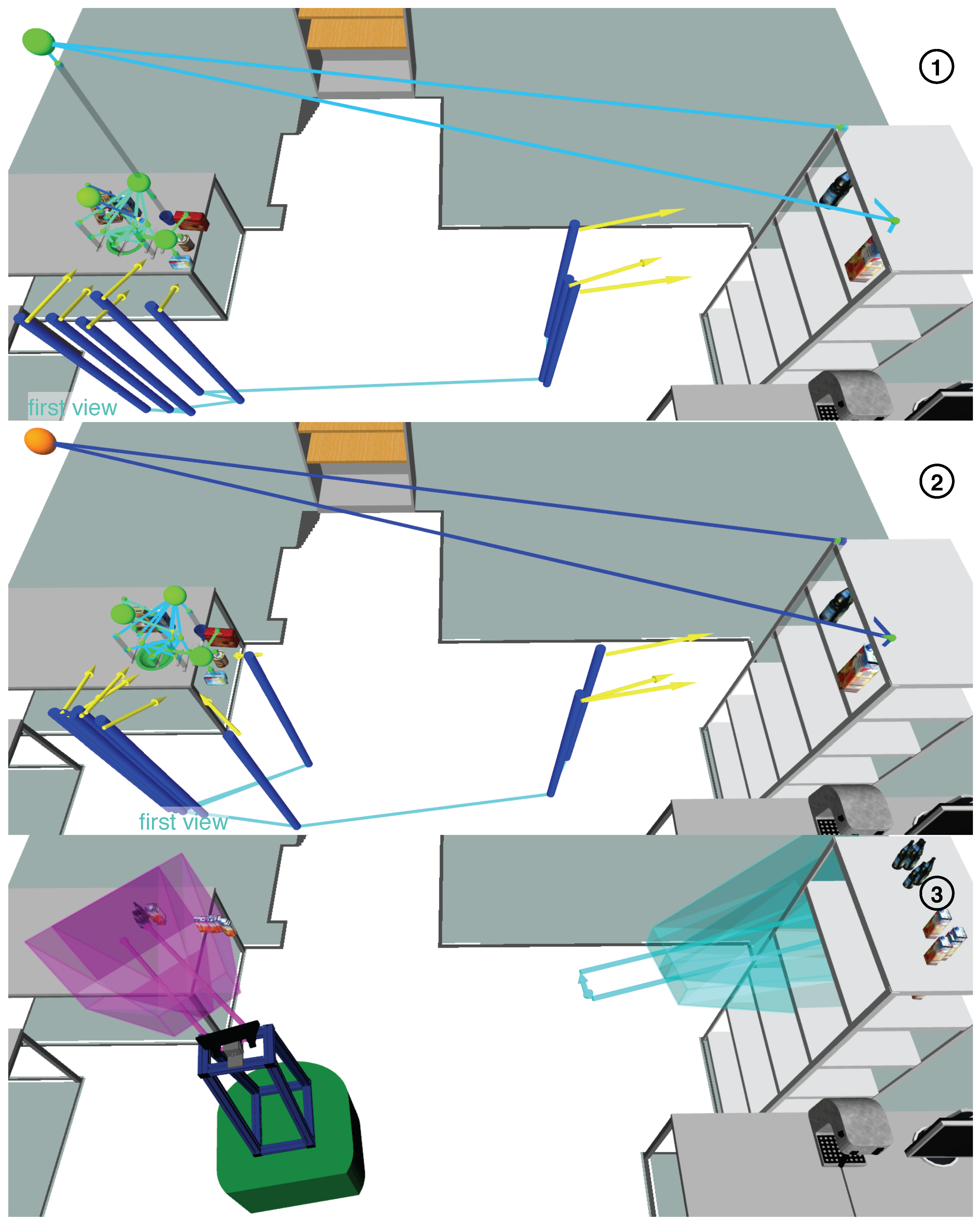
Figure 17.
Influence of object positions on pose prediction: Images 1 and 2 show s2_e1 and s2_e2, respectively. Between s2_e1 and s2_e2, all objects on the table were shifted to the right. Images 1 and 2: Recognized scenes and camera views MILD adopted. Image 3: Snapshot during the execution of s2_e2. The miniature objects correspond to predicted poses.
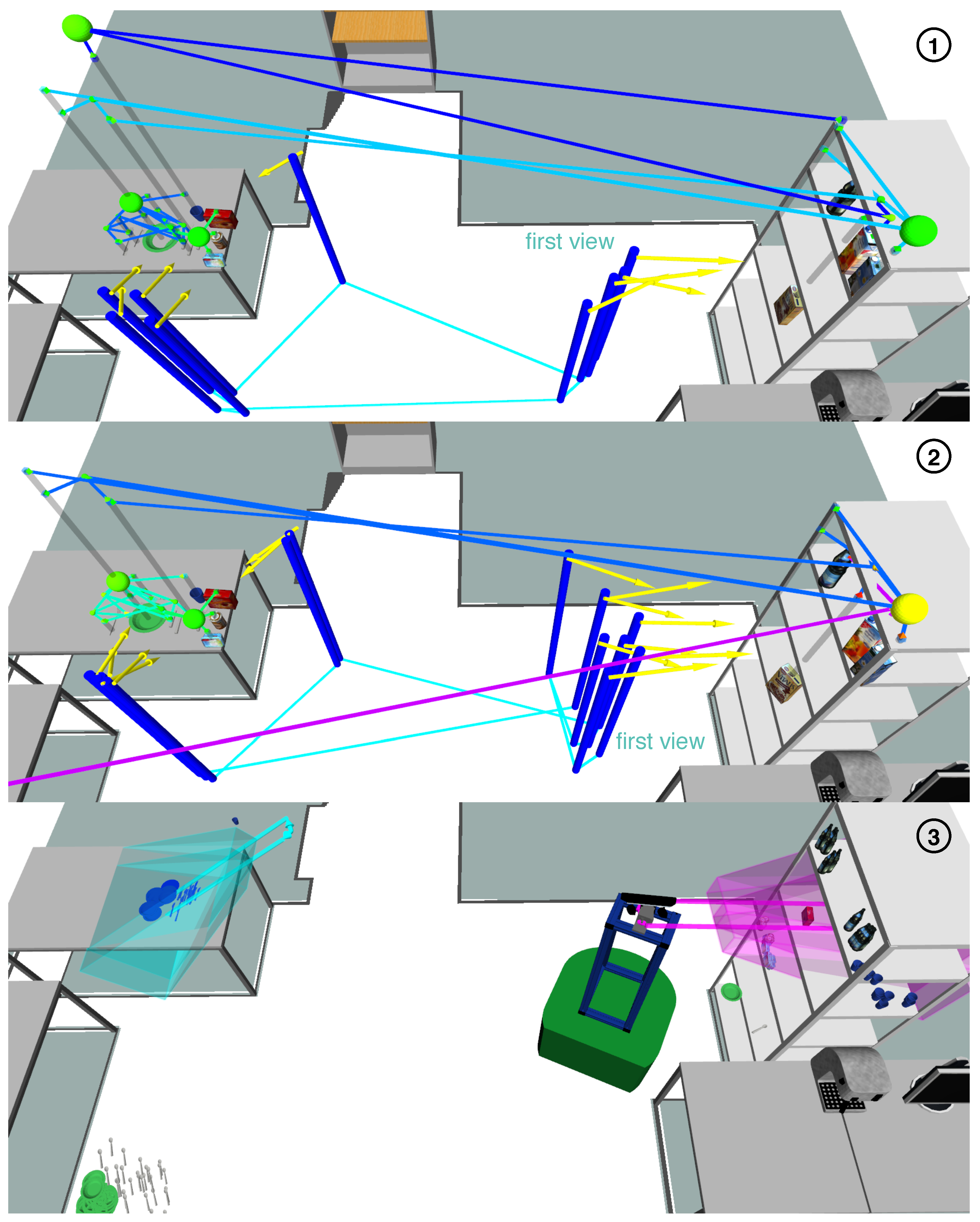
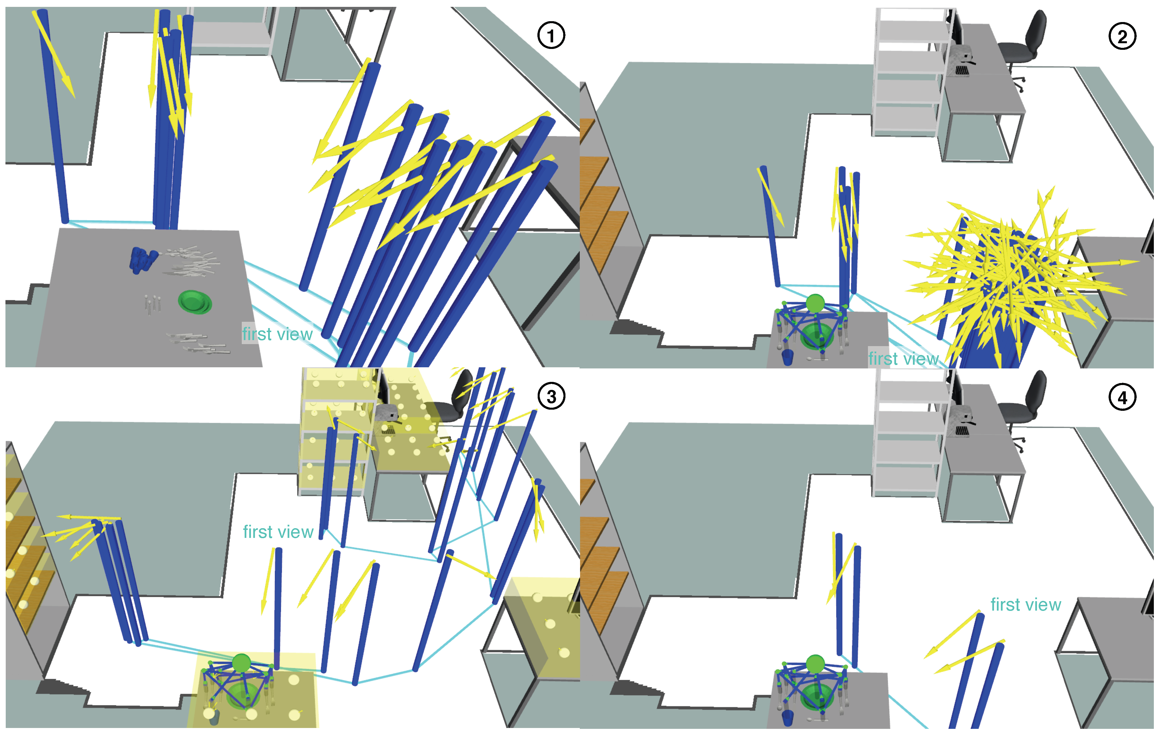
Figure 18.
Active scene recognition on a cluttered table. Image 1: Snapshot of physical objects. Image 2: Camera views adopted and recognized scene instances.
Figure 18.
Active scene recognition on a cluttered table. Image 1: Snapshot of physical objects. Image 2: Camera views adopted and recognized scene instances.
Figure 19.
Comparison of three approaches to ASR: For “direct search only” (images 1 and 2), “bounding box search” (image 3), and our ASR approach (image 4), we show which camera views were adopted. Additionally, image 1 shows demonstrated object poses, and images 2–4 show recognized scene instances.
Figure 20.
Times that our pose prediction algorithm took depending on the number of objects and trajectory length in the datasets.
Figure 20.
Times that our pose prediction algorithm took depending on the number of objects and trajectory length in the datasets.
Table 1.
We specify position and orientation compliances, as well as a similarity rating for all measured object poses, which ISM “Office_sub0” processed. The value of the recognition result’s objective function (returned by the ISM) is also provided. See
Section 5.2.2 for definitions of the objective function, rating, and compliances.
| Object Configuration | LeftScreen | RightScreen | Obj. Function |
|---|
| Simil. | Pos. | Orient. | Simil. | Pos. | Orient. |
|---|
| Correct configuration | 1.00 | 1.00 | 1.00 | 1.00 | 1.00 | 1.00 | 2.00 |
| RightScreen half-lowered | 1.00 | 1.00 | 1.00 | 0.72 | 0.72 | 1.00 | 1.72 |
| RightScreen fully lowered | 0.00 | 0.00 | 0.00 | 1.00 | 1.00 | 1.00 | 1.00 |
| LeftScreen half front | 1.00 | 1.00 | 1.00 | 0.60 | 0.61 | 0.98 | 1.60 |
| RightScreen half right | 1.00 | 1.00 | 1.00 | 0.96 | 0.97 | 0.99 | 1.96 |
| LeftScreen half-rotated | 0.54 | 0.93 | 0.58 | 1.00 | 1.00 | 1.00 | 1.54 |
| LeftScreen fully rotated | 0.00 | 0.00 | 0.00 | 1.00 | 1.00 | 1.00 | 1.00 |
| Mouse half right | 1.00 | 1.00 | 1.00 | 0.99 | 1.00 | 0.99 | 1.99 |
| Mouse half-rotated | 1.00 | 1.00 | 1.00 | 0.99 | 0.99 | 1.00 | 1.99 |
Table 2.
This table shows the same quantities as
Table 1, but this time for all measured object poses, which ISM “Office” processed. The same applies to the recognition result’s objective function.
Table 2.
This table shows the same quantities as
Table 1, but this time for all measured object poses, which ISM “Office” processed. The same applies to the recognition result’s objective function.
| Object Configuration | Keyboard | Mouse | Office_sub0 | Obj. Function |
|---|
| Simil. | Pos. | Orient. | Simil. | Pos. | Orient. | Simil. | Pos. | Orient. |
|---|
| Correct configuration | 0.98 | 0.98 | 1.00 | 1.00 | 1.00 | 1.00 | 2.00 | 1.00 | 1.00 | 3.98 |
| RightScreen half-lowered | 0.98 | 0.98 | 1.00 | 1.00 | 1.00 | 1.00 | 1.72 | 1.00 | 1.00 | 3.70 |
| RightScreen fully lowered | 1.00 | 1.00 | 1.00 | 1.00 | 1.00 | 1.00 | 1.00 | 1.00 | 1.00 | 3.00 |
| LeftScreen half front | 0.97 | 0.98 | 0.99 | 1.00 | 1.00 | 1.00 | 1.47 | 0.89 | 0.98 | 3.43 |
| RightScreen half right | 0.99 | 0.99 | 1.00 | 0.99 | 0.99 | 1.00 | 1.96 | 1.00 | 1.00 | 3.94 |
| LeftScreen half-rotated | 0.98 | 0.98 | 1.00 | 1.00 | 1.00 | 1.00 | 1.46 | 0.93 | 1.00 | 3.45 |
| LeftScreen fully rotated | 0.93 | 0.95 | 0.97 | 0.95 | 0.98 | 0.96 | 1.00 | 1.00 | 1.00 | 2.87 |
| Mouse half right | 0.99 | 0.99 | 1.00 | 0.86 | 0.86 | 1.00 | 1.99 | 1.00 | 1.00 | 3.83 |
| Mouse half-rotated | 1.00 | 1.00 | 1.00 | 0.77 | 1.00 | 0.78 | 1.96 | 0.98 | 0.99 | 3.73 |
Table 3.
Performance of ISM trees learned for scene categories in our kitchen and optimized by relation topology selection. Color coding as in
Table 1.
Table 3.
Performance of ISM trees learned for scene categories in our kitchen and optimized by relation topology selection. Color coding as in
Table 1.
| Scene Category | Trajectory Length | # Objects | Relations | numFPs() [%] | avgDur() [s] |
|---|
| Star | Optim. | Complete | Star | Optim. | Complete | Star | Optim. | Complete |
|---|
| Setting—Ready for Breakfast | 112 | 8 | 7 | 15 | 28 | 38.56 | 3.86 | 0 | 0.044 | 1.228 | 7.558 |
| Setting—Clear the Table | 220 | 8 | 7 | 15 | 28 | 19.59 | 2.92 | 0 | 0.196 | 2.430 | 8.772 |
| Cupboard—Filled | 103 | 9 | 8 | 15 | 36 | 23.70 | 8.09 | 0 | 0.020 | 0.140 | 1.070 |
| Dishwasher Basket—Filled | 117 | 10 | 9 | 9 | 45 | 15.38 | 0 | 0 | 0.053 | 0.060 | 1.099 |
| Sandwich—Setting | 92 | 5 | 4 | 4 | 10 | 0 | 0 | 0 | 0.019 | 0.019 | 0.131 |
| Sandwich—On Shelf | 98 | 6 | 5 | 7 | 15 | 29.05 | 6.70 | 0 | 0.017 | 0.042 | 0.264 |
| Drinks—Setting | 23 | 3 | 2 | 2 | 3 | 67.02 | 67.02 | 0 | 0.001 | 0.001 | 0.004 |
| Drinks—On Shelf | 44 | 4 | 3 | 3 | 6 | 44.51 | 11.54 | 0 | 0.003 | 0.008 | 0.013 |
| Cereals—Setting | 52 | 4 | 3 | 3 | 6 | 33.67 | 0 | 0 | 0.002 | 0.004 | 0.012 |
| Cereals—On Shelf | 98 | 5 | 4 | 7 | 10 | 9.50 | 1.68 | 0 | 0.014 | 0.053 | 0.181 |
Table 4.
Performance measures for experiments with the physical MILD robot, which were used to evaluate active scene recognition. Color coding as in
Table 1.
Table 4.
Performance measures for experiments with the physical MILD robot, which were used to evaluate active scene recognition. Color coding as in
Table 1.
| Task | Duration [s] | Camera
Views | Found Objects [%] | Confidences |
|---|
| Setting | Drinks | Cereals | Sandwich |
|---|
| Ready | Setting | on Shelf | Setting | on Shelf | Setting | on Shelf |
|---|
| s1_e1 | 783.96 | 16 | 100 | 0.97 | 0.33 | 0.99 | 0.49 | 0.85 | 0.99 | 0.34 |
| | 425.63 | 9 | 100 | 0.99 | 0.47 | 0.97 | 0.48 | 0.99 | 1.00 | 0.37 |
| s1_e2 | 560.18 | 12 | 100 | 0.97 | 0.33 | 0.42 | 0.46 | 0.82 | 0.99 | 0.49 |
| | 562.46 | 14 | 100 | 0.97 | 0.33 | 0.41 | 0.47 | 0.89 | 0.99 | 0.49 |
| s2_e1 | 367.32 | 8 | 100 | 0.93 | 0.33 | 0.98 | 0.96 | 0.75 | 1.00 | 0.45 |
| | 336.18 | 8 | 100 | 0.91 | 0.33 | 0.98 | 0.96 | 0.74 | 0.99 | 0.50 |
| s2_e2 | 584.07 | 13 | 100 | 0.95 | 0.33 | 0.73 | 0.97 | 0.68 | 0.99 | 0.34 |
| | 434.99 | 10 | 100 | 0.92 | 0.33 | 0.75 | 0.98 | 0.69 | 1.00 | 0.42 |
| s3_e1 | 533.29 | 11 | 93.75 | 0.99 | 0.93 | 0.25 | 0.99 | 0.50 | 1.00 | 0.34 |
| | 439.61 | 8 | 100 | 0.99 | 0.91 | 0.48 | 0.98 | 0.75 | 1.00 | 0.37 |


