
A Comprehensive Multibody Model of a Collaborative Robot to Support Model-Based Health Management

 ,
,  ,
,  ,
, 
 and
and 
Abstract
1. Introduction
2. Mathematical Model of the UR5
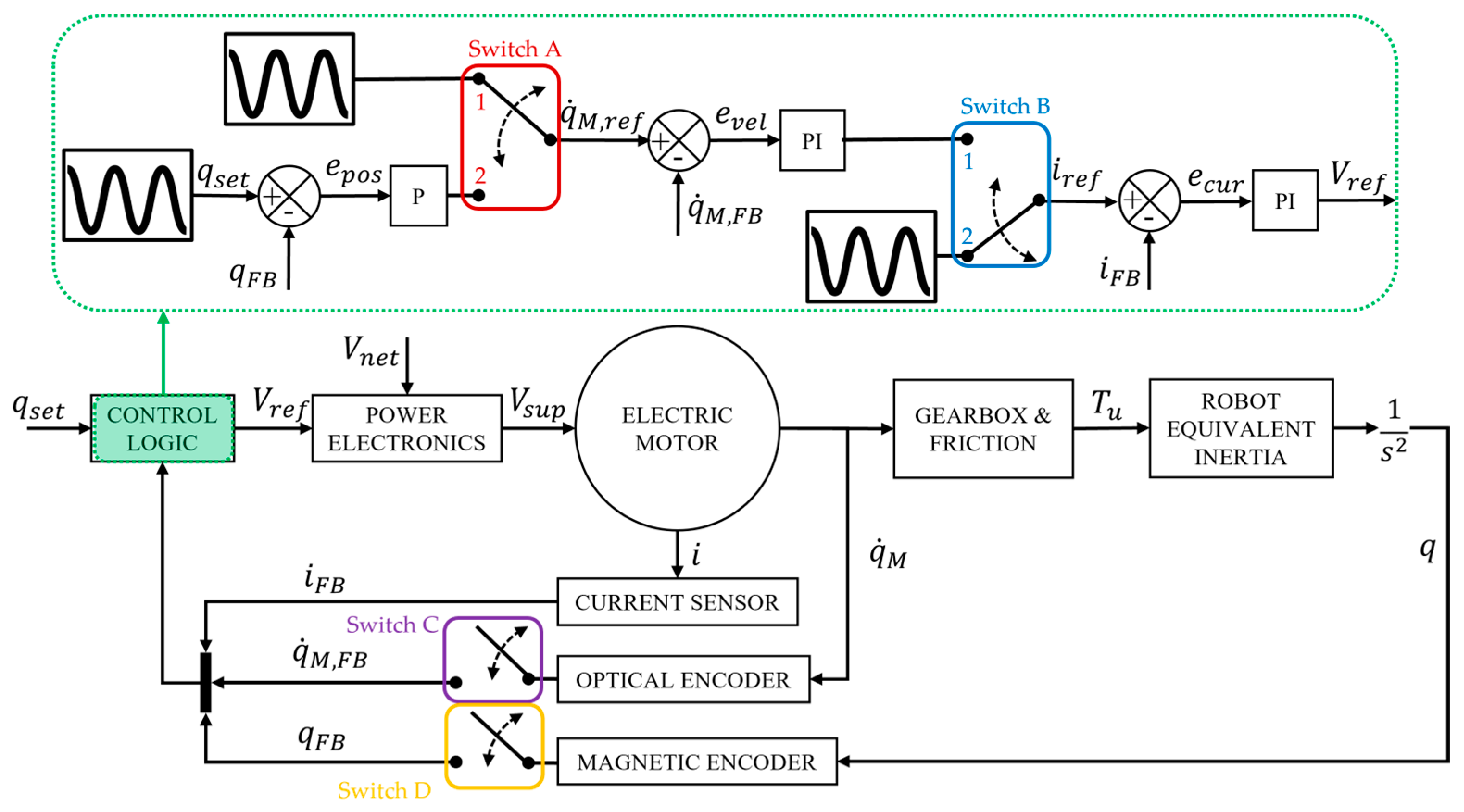
2.1. Control Logic and Power Electronics
2.2. Electric Motor
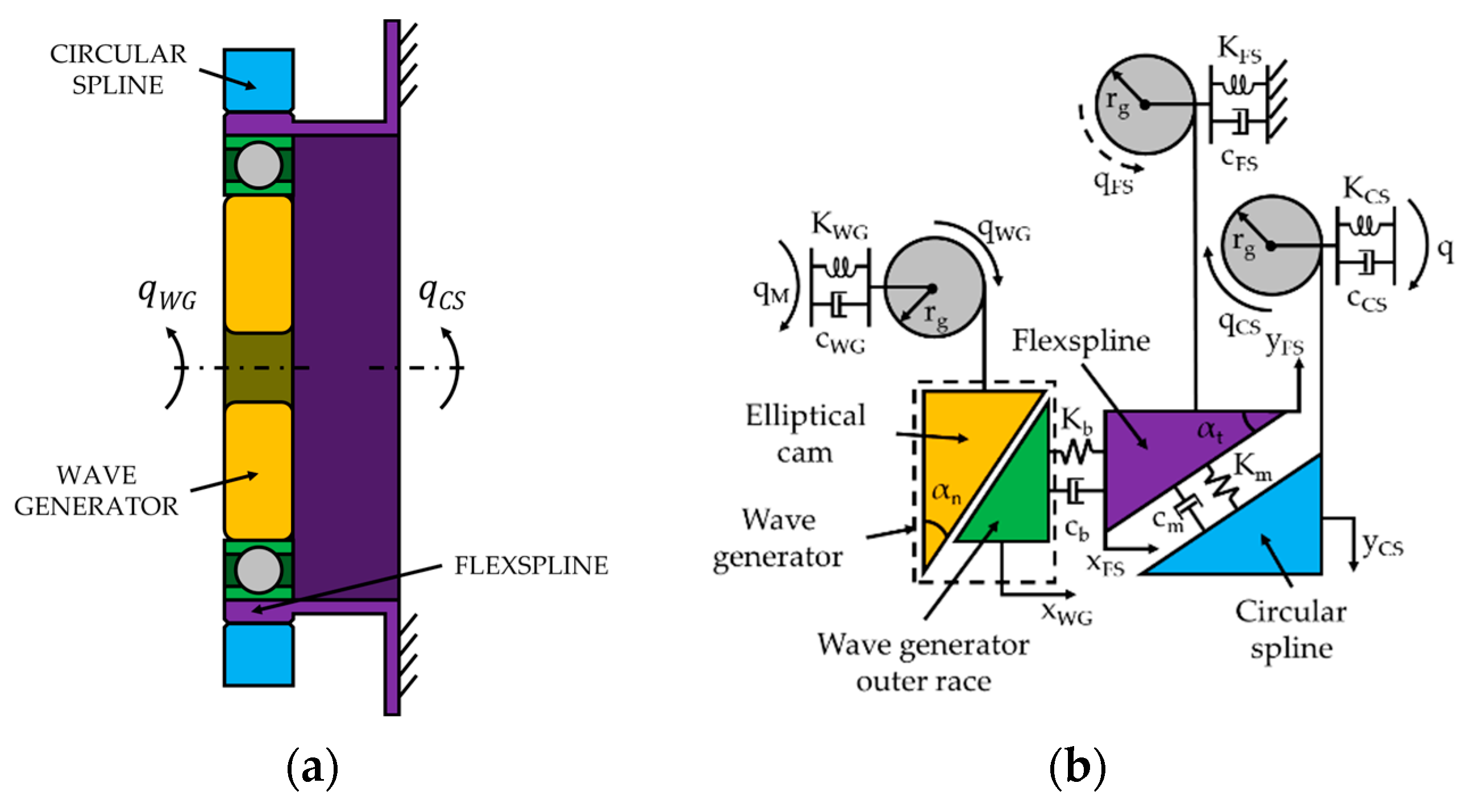
2.3. Gearbox
- Group 1: comprised of the first four equations describing, respectively, the dynamic equilibrium of the wave generator, the flexspline radial and tangential contributions, and the one of the circular spline;
- Group 2: comprised of the last five equations, representing the interactions between the input shaft and the elliptical cam, through the WG bearing, between the FS and the CS teeth, and between the FS and the joint case and the CS with the output shaft.
2.4. Friction
2.5. Sensors
- Optical encoder: an encoder integral to the motor/input shaft used to derive the motor angular velocity () used to provide the feedback signal () to the velocity control loop;
- Magnetic encoder: an encoder integral to the joint/output shaft used to measure the joint actual angular position () used to close the position control loop through the feedback signal ();
- Current sensor: used to measure the motor current () necessary to close the current control loop through the feedback signal ().
2.6. Six-DoF Forward Kinematics and Dynamics
3. Experimental Testing
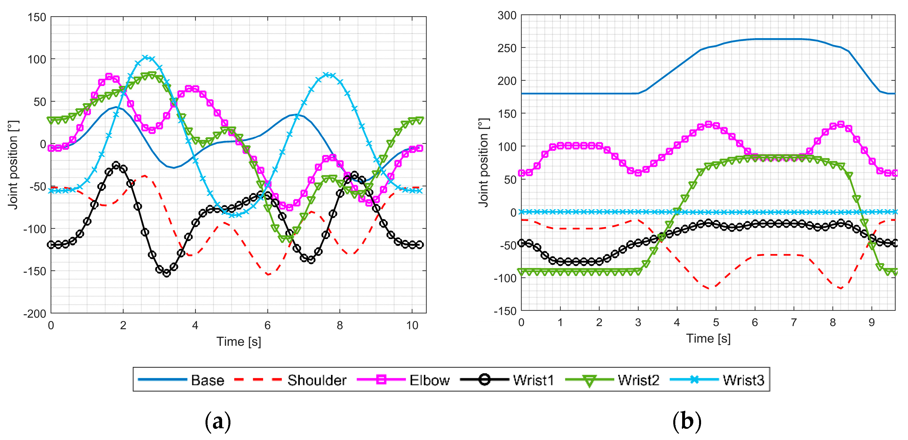
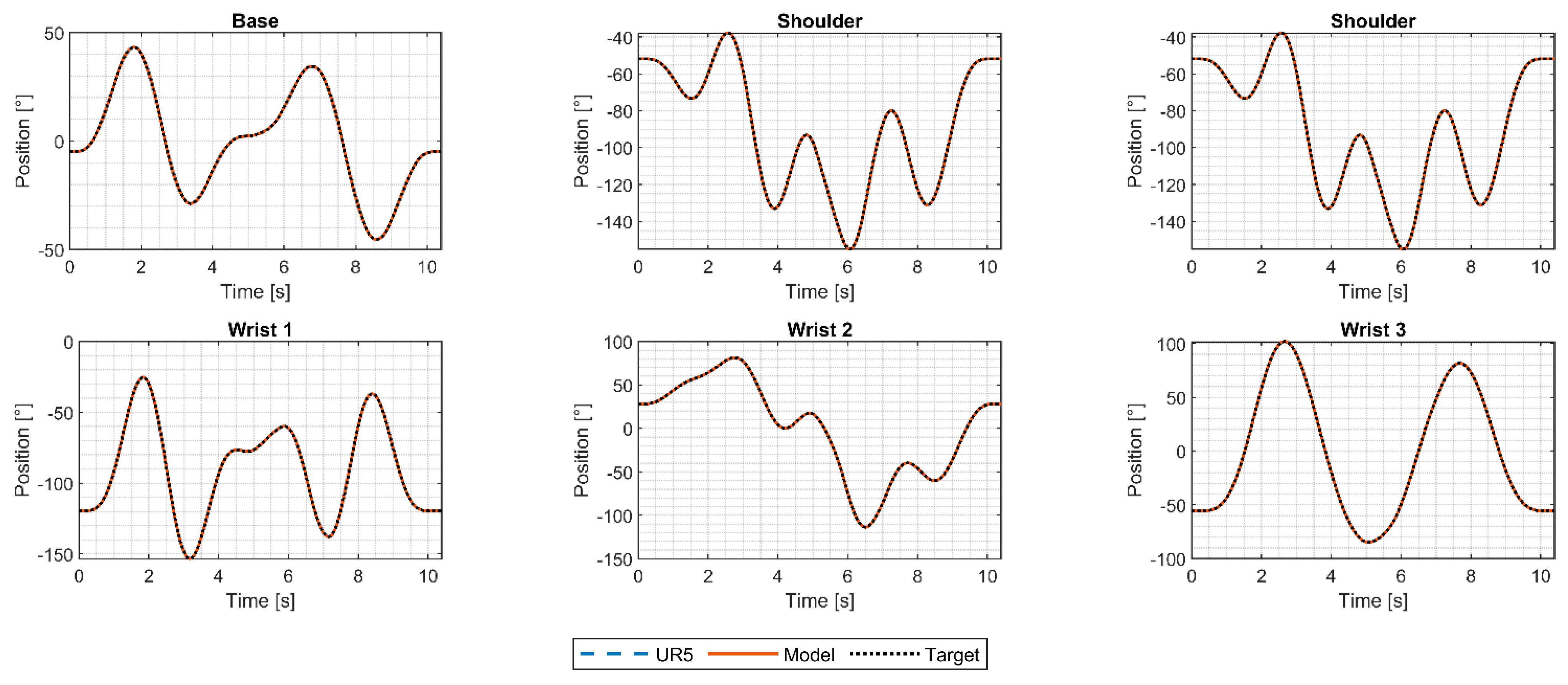
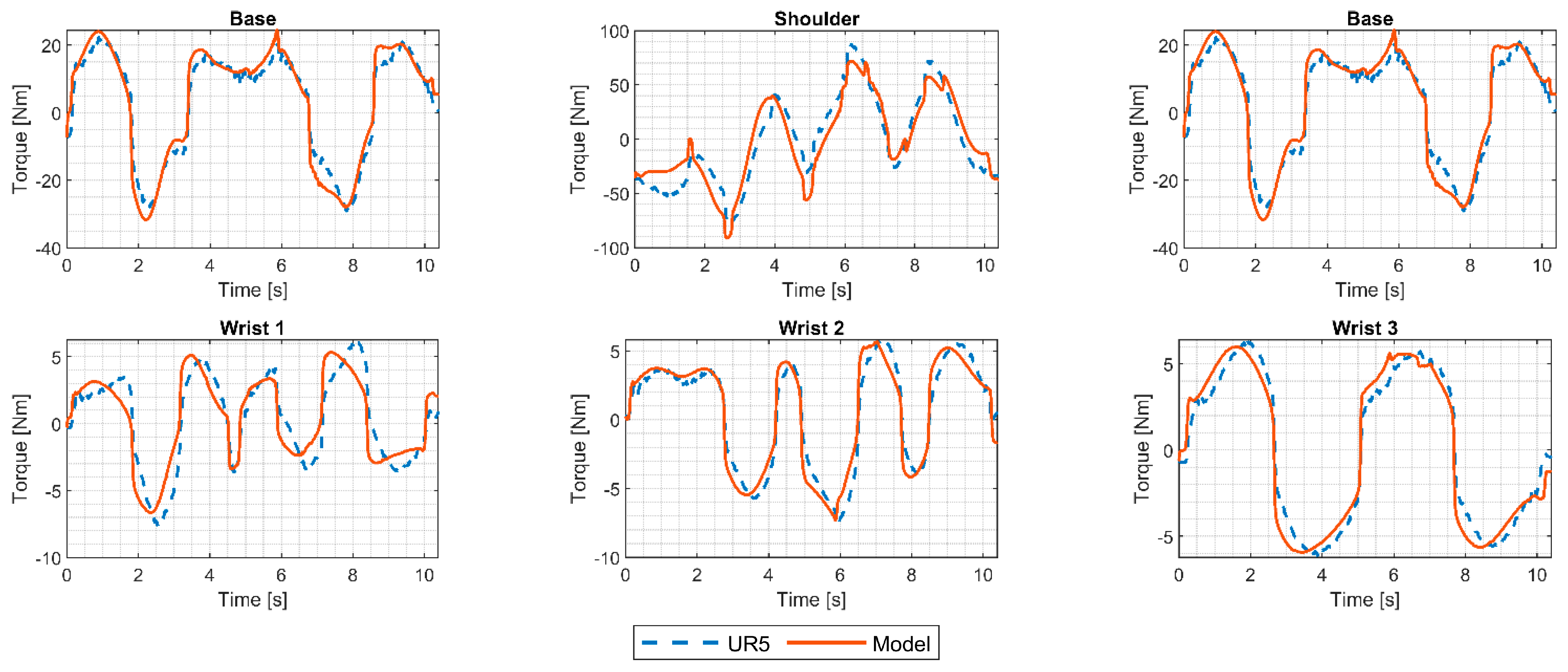
3.1. Dynamic Parameters Excitation Trajectory
- Implementation of simplified DC models of the joint motors instead of using three-phase ones, whose parameters, such as resistance and inductance, are not fully known. Moreover, the motor back-EMF constant () was assumed to be constant for the entire trajectory, while it slightly changes with the applied load.
- A possible incorrect description of the joint friction. As already mentioned, the identification algorithms provided by [40,52] only take into account viscous and Coulomb friction, while they are not able to describe more complex trends, such as the ones affecting the real robot. To do so, friction was modeled through Equation (7), whose coefficients were tuned according to several experimental campaigns aiming to reach a good overall fit between simulated and measured motor currents.
- Lack of both the kinematic error and the gear torsional hysteresis in the translation-equivalent models of the strain wave gears.
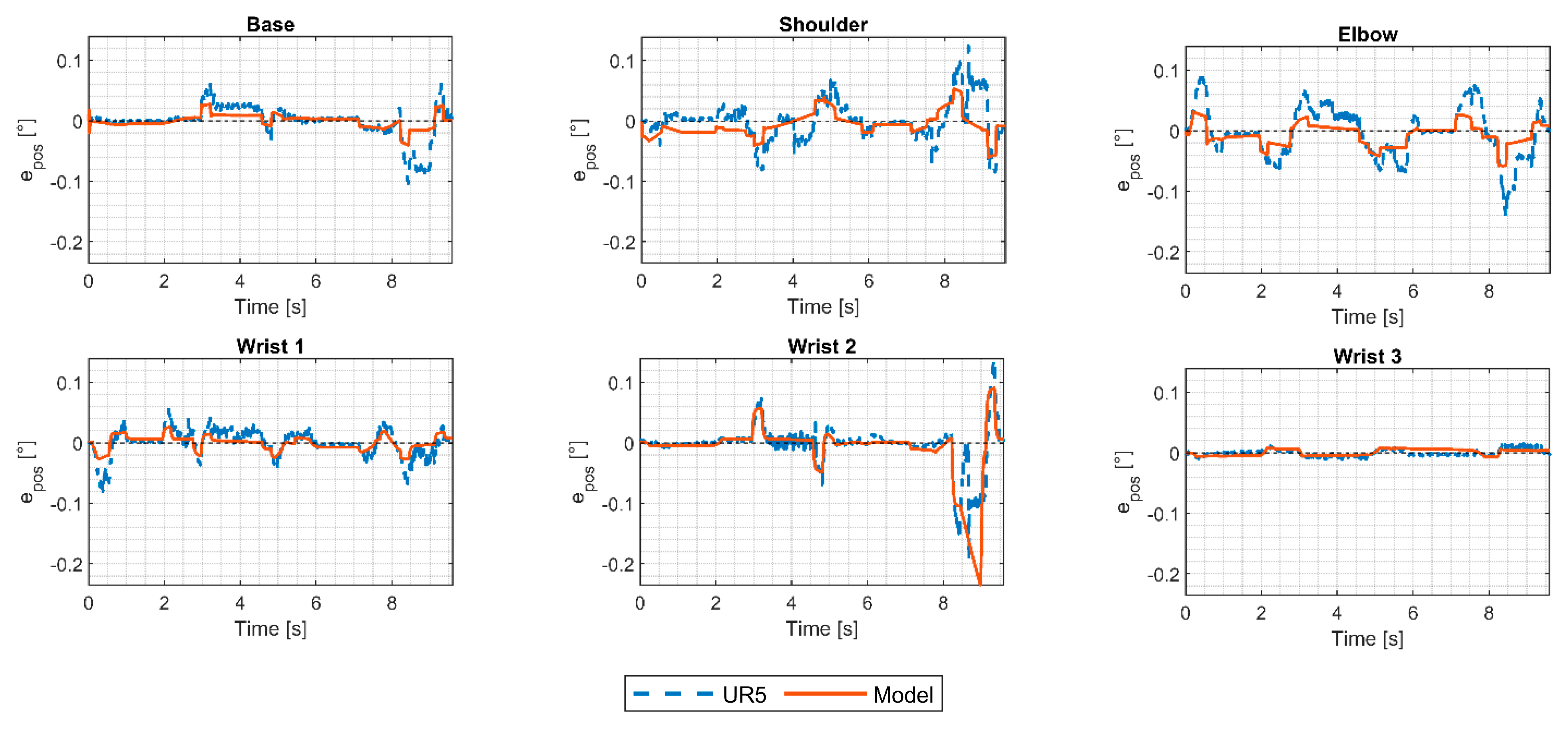
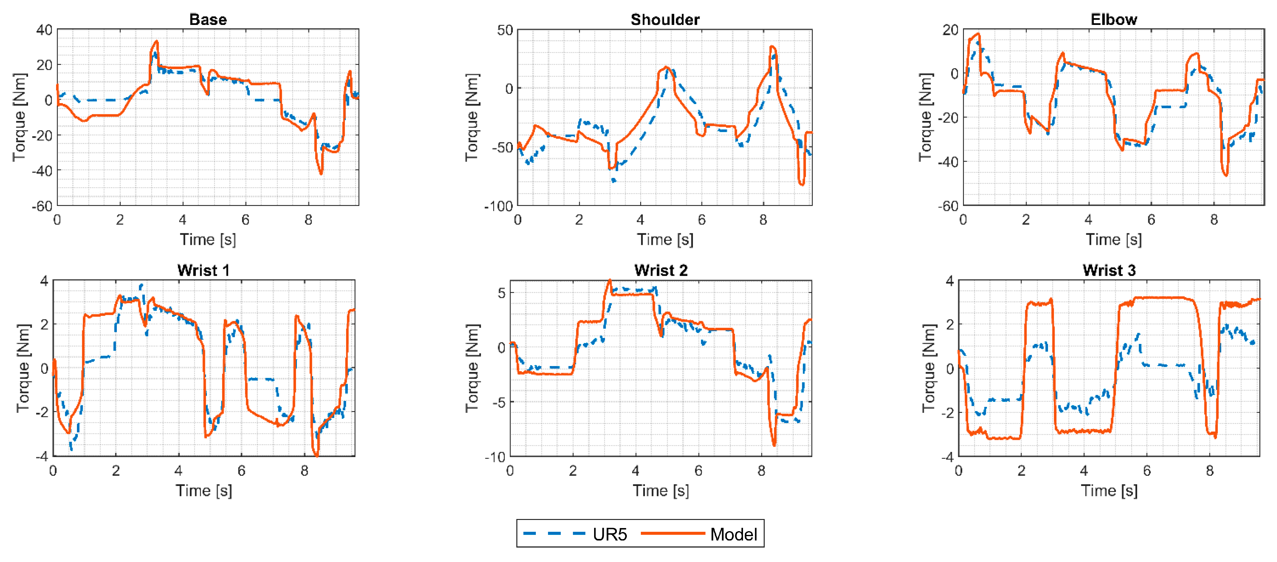
- The joint control logic schematized in Figure 2 is not the same as the one implemented in the real robot, which is unknown. As an example, studies such as [69,70] highlight how manipulators from Universal Robots are equipped with vibration suppression algorithms, which were not implemented in the current model. Having two different control logics deeply affects the torque trends. Since, according to the scheme reported in Figure 2, the current control loop is the most internal one, the reference value of the motor current is affected by both the position and the velocity control loops. As a direct consequence, since, as depicted in Figure 8, the joint position error is different between the two manipulators, the velocity reference signal will also be different. Hence, based on the adopted PI gains, the motor angular velocity error differs from the one of the real robot as well.
- While the control parameters reported in Table 1 are constant, it should not be excluded that Universal Robots A/S might adopt variable settings according to the specific operating conditions of the manipulator. such as very fast or very slow movements.
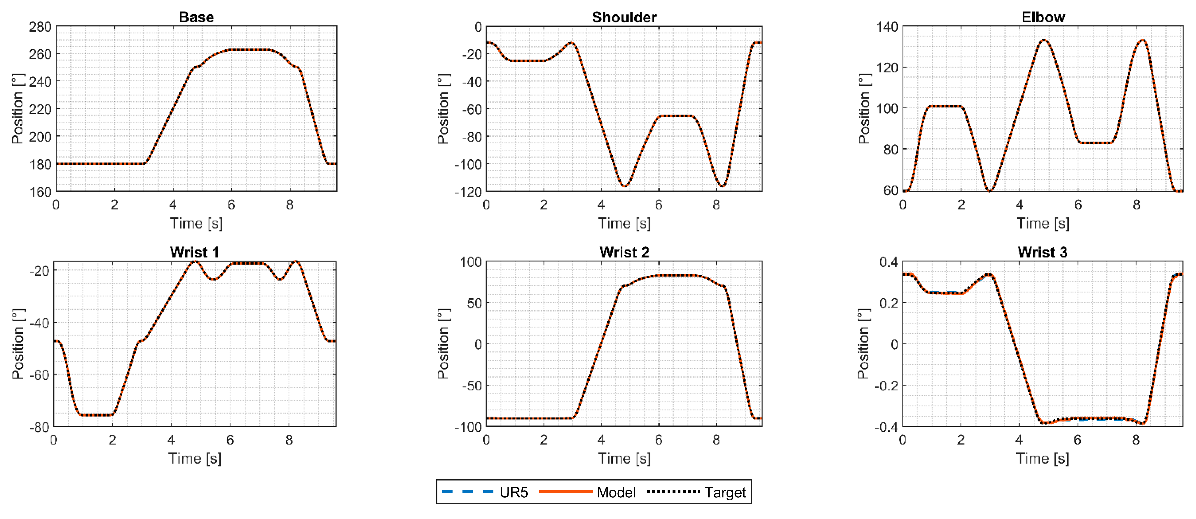
3.2. Pick-and-Place Trajectory
4. Conclusions
Author Contributions
Funding
Conflicts of Interest
Nomenclature
| Symbol | Name | Symbol | Name |
| Joint position | Teeth pressure angle | ||
| Joint set position | WG torsional stiffness | ||
| Joint feedback position | WG damping coefficient | ||
| Joint position error | Bearing radial stiffness | ||
| Motor velocity | Bearing radial damping coefficient | ||
| Motor reference velocity | FS torsional stiffness | ||
| Motor feedback velocity | FS damping coefficient | ||
| Motor velocity error | Meshing stiffness between FS and CS | ||
| Motor current | Meshing damping coefficient | ||
| Motor reference current | CS torsional stiffness | ||
| Motor feedback current | CS damping coefficient | ||
| Motor current error | Gear ratio | ||
| Reference voltage | WG inertia | ||
| Supply voltage | FS inertia | ||
| Network voltage | CS inertia | ||
| DC motor equivalent inductance | WG angular position | ||
| DC motor equivalent resistance | CS angular position | ||
| Motor torque constant | Radial displacement of the bearing outer rings | ||
| Motor voltage constant | Radial displacement of the FS | ||
| Motor electromechanical torque | Tangential displacement of the FS free edge | ||
| Motor rotor moment of inertia | Tangential displacement of the CS | ||
| Strain wave gear input torque | Joint friction torque | ||
| Strain wave gear output torque | Static friction torque | ||
| Strain wave gear primitive equivalent radius | Coulomb friction torque | ||
| FS teeth number | Viscous friction coefficient | ||
| CS teeth number | Joint useful torque |
Appendix A

- Current loop: switch A not influent, switch B in position 2, switches C and D open;
- Velocity loop: switches A and B both in position 1, switch C closed, switch D open;
- Position loop: switch A in position 2 and switch B in position 1, switches C and D closed.


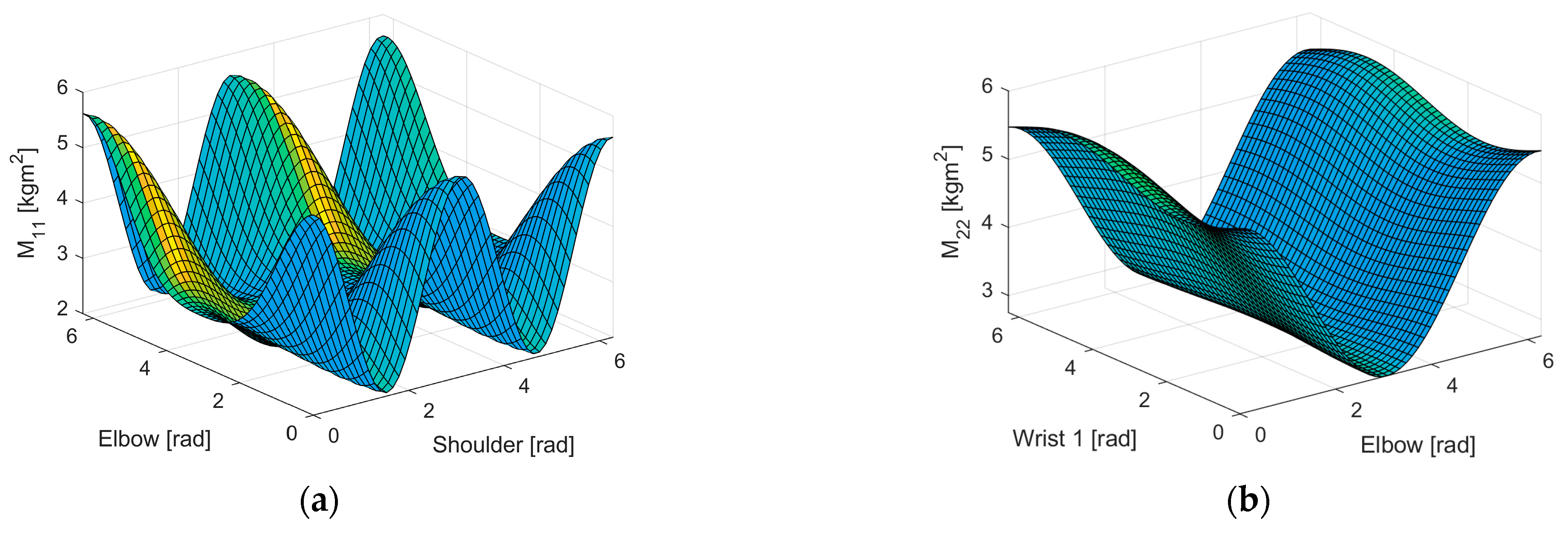
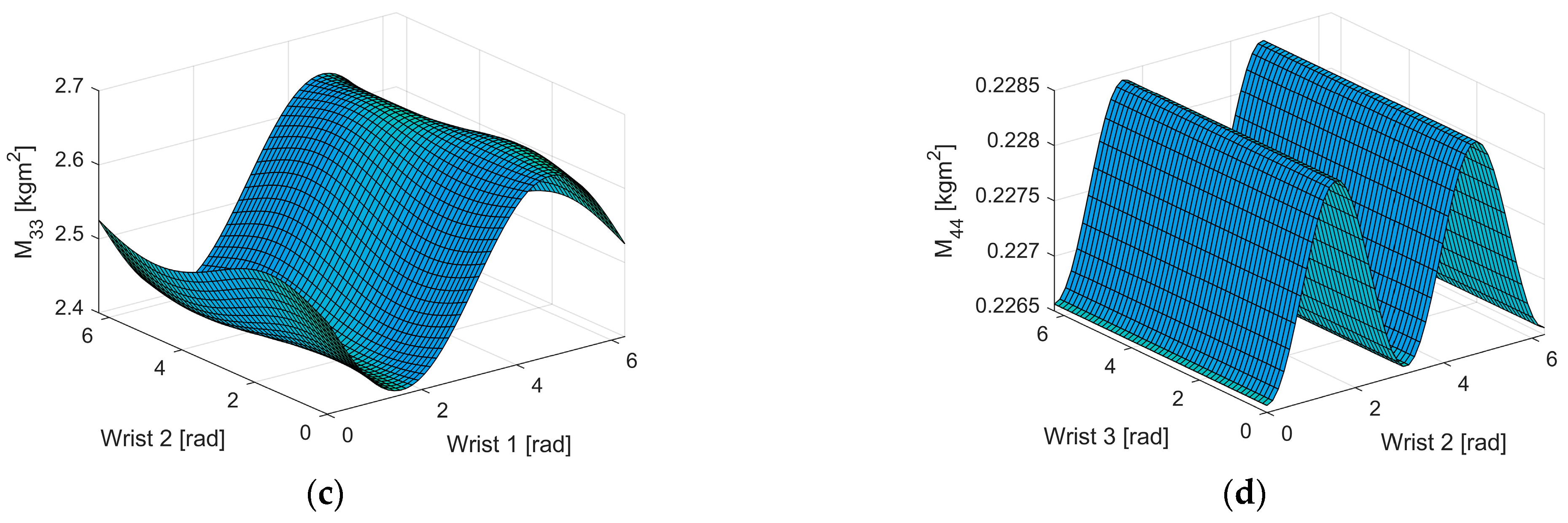
| [kgm2] | Base | Shoulder | Elbow | Wrist 1 | Wrist 2 | Wrist 3 |
|---|---|---|---|---|---|---|
| Maximum | 5.628 | 5.719 | 2.649 | 0.228 | 0.215 | 0.212 |
| Mean | 3.194 | 4.144 | 2.526 | 0.227 | 0.215 | 0.212 |
| Minimum | 2.061 | 2.752 | 2.405 | 0.226 | 0.215 | 0.212 |
References
- International Federation of Robotics. The Impact of Robots on Productivity, Employment and Jobs; International Federation of Robotics: Frankfurt, Germany, 2017. [Google Scholar]
- Matheson, E.; Minto, R.; Zampieri, E.G.G.; Faccio, M.; Rosati, G. Human-Robot Collaboration in Manufacturing Applications: A Review. Robotics 2019, 4, 100. [Google Scholar] [CrossRef]
- González, J.C.; Martínez, S.; Jardón, A.; Balaguer, C. Robot-aided tunnel inspection and maintenance system. In Proceedings of the 26th International Symposium on Automation and Robotics in Construction, ISARC 2009, Austin, TX, USA, 24–27 June 2009; pp. 420–426. [Google Scholar]
- Raviola, A.; Antonacci, M.; Marino, F.; Jacazio, G.; Sorli, M.; Wende, G. Collaborative robotics: Enhance maintenance procedures on primary flight control servo-actuators. Appl. Sci. 2021, 11, 4929. [Google Scholar] [CrossRef]
- Parker, L.E.; Draper, J.V. Robotics applications in maintenance and repair. In Handbook of Industrial Robotics; Wiley Online Books: Hoboken, NJ, USA, 1998; p. 1378. ISBN 0471177830. [Google Scholar]
- Abdi, H.; Nahavandi, S.; Frayman, Y.; Maciejewski, A.A. Optimal mapping of joint faults into healthy joint velocity space for fault-tolerant redundant manipulators. Robotica 2011, 30, 671. [Google Scholar] [CrossRef]
- Pinto, R.; Cerquitelli, T. Robot fault detection and remaining life estimation for predictive maintenance. Procedia Comput. Sci. 2019, 151, 709–716. [Google Scholar] [CrossRef]
- Liu, H.; Wei, T.; Wang, X. Signal Decomposition and Fault Diagnosis of a SCARA Robot Based Only on Tip Acceleration Measurement. In Proceedings of the 2009 International Conference on Mechatronics and Automation (ICMA 2009), Changchun, China, 9–12 August 2009; pp. 4811–4816. [Google Scholar] [CrossRef]
- De Martin, A.; Jacazio, G.; Nesci, A.; Sorli, M. In-depth Feature Selection for PHM System’s Feasibility Study for Helicopters’ Main and Tail Rotor Actuators. In Proceedings of the European Conference of the PHM Society 2020, Turin, Italy, 27–31 July 2020; pp. 1–9. [Google Scholar]
- De Martin, A.; Jacazio, G.; Vachtsevanos, G. Windings Fault Detection and Prognosis in Electro-Mechanical Flight Control Actuators Operating in Active-Active Configuration. Int. J. Progn. Health Manag. 2017, 8. [Google Scholar] [CrossRef]
- Raviola, A.; De Martin, A.; Guida, R.; Jacazio, G.; Mauro, S.; Sorli, M. Harmonic Drive Gear Failures in Industrial Robots Applications: An Overview. In Proceedings of the European Conference of the PHM Society 2021, Online, 6–8 July 2021. [Google Scholar]
- Jaber, A.A.; Bicker, R. Fault Diagnosis of Industrial Robot Bearings Based on Discrete Wavelet Transform and Artificial Neural Network. Insight-Non-Destr. Test. Cond. Monit. 2016, 58, 179–186. [Google Scholar] [CrossRef]
- Kdqj, H.; Pdqglqh, P.; Vxq, K.; Dee, F.Q.; Lqfoxglqj, P.; Sh, V.W.; Dqg, V.; Wudfwlrq, I.H.; Vroxwlrq, S.; Yhulilhg, L.V.; et al. Health Monitoring of Strain Wave Gear on Industrial Robots. In Proceedings of the IEEE 8th Data Driven Control and Learning Systems Conference, Dali, China, 24–27 May 2019; pp. 1166–1170. [Google Scholar]
- Yang, G.; Zhong, Y.; Yang, L.; Du, R. Fault Detection of Harmonic Drive Using Multiscale Convolutional Neural Network. IEEE Trans. Instrum. Meas. 2021, 70, 1–11. [Google Scholar] [CrossRef]
- Yang, G.; Zhong, Y.; Yang, L.; Tao, H.; Li, J.; Du, R. Fault Diagnosis of Harmonic Drive with Imbalanced Data Using Generative Adversarial Network. IEEE Trans. Instrum. Meas. 2021, 70, 1–11. [Google Scholar] [CrossRef]
- Raouf, I.; Lee, H.; Noh, Y.R.; Youn, B.D.; Kim, H.S. Prognostic health management of the robotic strain wave gear reducer based on variable speed of operation: A data-driven via deep learning approach. J. Comput. Des. Eng. 2022, 1775–1788. [Google Scholar] [CrossRef]
- Zhou, Q.; Wang, Y.; Jianming, X. A Summary of Health Prognostics Methods for Industrial Robots. In Proceedings of the 2019 Prognostics & System Health Management Conference, Qingdao, China, 25–27 October 2019; pp. 5–10. [Google Scholar]
- Qiao, G.; Weiss, B.A. Accuracy degradation analysis for industrial robot systems. In Proceedings of the ASME 2017 12th International Manufacturing Science and Engineering Conference, MSEC 2017 collocated with the JSME/ASME 2017 6th International Conference on Materials and Processing, Los Angeles, CA, USA, 4–8 June 2017; Volume 3, p. 9. [Google Scholar]
- Majid, M.A.A.; Fudzin, F. Study on robots failures in automotive painting line. ARPN J. Eng. Appl. Sci. 2017, 12, 62–67. [Google Scholar]
- Grosso, L.A.; De Martin, A.; Jacazio, G.; Sorli, M. Development of data-driven PHM solutions for robot hemming in automotive production lines. Int. J. Progn. Health Manag. 2020, 11. [Google Scholar]
- Aivaliotis, P.; Georgoulias, K.; Chryssolouris, G. The use of Digital Twin for predictive maintenance in manufacturing. Int. J. Comput. Integr. Manuf. 2019, 32, 1067–1080. [Google Scholar] [CrossRef]
- Guida, R.; De Simone, M.C.; Dašić, P.; Guida, D. Modeling techniques for kinematic analysis of a six-axis robotic arm. IOP Conf. Ser. Mater. Sci. Eng. 2019, 568, 012115. [Google Scholar]
- Kardoš, J. The Simplified Dynamic Model of a Robot Manipulator. In Proceedings of the 18th International Conference on Technical Computing, Bratislava, Slovakia, 8–10 January 2010; Volume 1, pp. 1–6. [Google Scholar]
- Liang, B.; Cheng, Y.; Zhu, X.; Liu, H.; Wang, X. Calibration of UR5 manipulator based on kinematic models. In Proceedings of the 30th Chinese Control and Decision Conference, CCDC 2018, Shenyang, China, 9–11 June 2018; pp. 3552–3557. [Google Scholar]
- Kebria, P.M.; Al-Wais, S.; Abdi, H.; Nahavandi, S. Kinematic and dynamic modelling of UR5 manipulator. In Proceedings of the International Conference on Systems, Man, and Cybernetics, SMC 2016, Budapest, Hungary, 9–12 October 2016; pp. 4229–4234. [Google Scholar]
- Kovincic, N.; Müller, A.; Gattringer, H.; Weyrer, M.; Schlotzhauer, A.; Brandstötter, M. Dynamic parameter identification of the Universal Robots UR5. In Proceedings of the Austrian Robotics Workshop and OAGM Joint Workshop on Vision and Robotics, Steyr, Austria, 9–10 May 2019. [Google Scholar]
- Boscariol, P.; Caracciolo, R.; Richiedei, D.; Trevisani, A. Energy Optimization of Functionally Redundant Robots through Motion Design. Appl. Sci. 2020, 10, 3022. [Google Scholar] [CrossRef]
- Paryanto; Brossog, M.; Bornschlegl, M.; Franke, J. Reducing the energy consumption of industrial robots in manufacturing systems. Int. J. Adv. Manuf. Technol. 2015, 78, 1315–1328. [Google Scholar] [CrossRef]
- Bilberg, A.; Malik, A.A. Digital twin driven human–robot collaborative assembly. CIRP Ann. 2019, 68, 499–502. [Google Scholar] [CrossRef]
- Weistroffer, V.; Keith, F.; Bisiaux, A.; Andriot, C.; Lasnier, A. Using Physics-Based Digital Twins and Extended Reality for the Safety and Ergonomics Evaluation of Cobotic Workstations. Front. Virtual Real. 2022, 3, 18. [Google Scholar] [CrossRef]
- Leboutet, Q.; Roux, J.; Janot, A.; Guadarrama-Olvera, J.R.; Cheng, G. Inertial Parameter Identification in Robotics: A Survey. Appl. Sci. 2021, 11, 4303. [Google Scholar] [CrossRef]
- Bejczy, A.K. Robot Arm Dynamics and Control (No. NASA-CR-136935). 1974. Available online: https://ntrs.nasa.gov/citations/19740008732 (accessed on 25 April 2023).
- Wahyuningtri, S.; Adzkiya, D.; Nurhadi, H. Motion Control Design and Analysis of UR5 Collaborative Robots Using Proportional Integral Derivative (PID) Method. In Proceedings of the International Conference on Advanced Mechatronics, Intelligent Manufacture and Industrial Automation, Surabaya, Indonesya, 8–9 December 2021; pp. 157–161. [Google Scholar]
- Sheng, B.; Meng, W.; Deng, C.; Xie, S. Model based kinematic & dynamic simulation of 6-DOF upper-limb rehabilitation robot. In Proceedings of the 2016 Asia-Pacific Conference on Intelligent Robot Systems, Tokyo, Japan, 20–22 July 2016; pp. 21–25. [Google Scholar]
- Good, M.C.; Sweet, L.M.; Strobel, K.L. Dynamic models for control system design of integrated robot and drive systems. J. Dyn. Syst. Meas. Control. Trans. ASME 1985, 107, 53–59. [Google Scholar] [CrossRef]
- Abedinifar, M.; Ertugrul, S.; Arguz, S.H. Nonlinear model identification and statistical verification using experimental data with a case study of the UR5 manipulator joint parameters. Robotica 2022, 41, 1348–1370. [Google Scholar] [CrossRef]
- Tarn, T.-J.; Bejczy, A.K.; Yun, X.; Li, Z. Effect of Motor Dynamics on Nonlinear Feedback Rotor Arm Control. In Proceedings of the IEEE Transactions on Robotics and Automation, Sacramento, CA, USA, 7–12 April 1991; Volume 7, pp. 1–9. [Google Scholar]
- Wu, W.; Zhu, S.; Wang, X.; Liu, H. Closed-loop dynamic parameter identification of robot manipulators using modified fourier series. Int. J. Adv. Robot. Syst. 2012, 9, 45818. [Google Scholar] [CrossRef]
- Qin, Z.; Baron, L.; Birglen, L. A new approach to the dynamic parameter identification of robotic manipulators. Robotica 2010, 28, 539–547. [Google Scholar] [CrossRef]
- Raviola, A.; Guida, R.; De Martin, A.; Pastorelli, S.; Mauro, S.; Sorli, M. Effects of temperature and mounting configuration on the dynamic parameters identification of industrial robots. Robotics 2021, 10, 83. [Google Scholar] [CrossRef]
- Wang, S.; Deng, X.; Feng, H.; Ren, K.; Li, F.; Liu, Y. Dynamic simulation analysis and experimental study of an industrial robot with novel joint reducers. Multibody Syst. Dyn. 2023, 57, 107–131. [Google Scholar] [CrossRef]
- Zhang, D.; Li, X.; Yang, M.; Wang, F.; Han, X. Non-random vibration analysis of rotate vector reducer. J. Sound Vib. 2023, 542, 117380. [Google Scholar] [CrossRef]
- Xu, L.X.; Chen, B.K.; Li, C.Y. Dynamic modelling and contact analysis of bearing-cycloid-pinwheel transmission mechanisms used in joint rotate vector reducers. Mech. Mach. Theory 2019, 137, 432–458. [Google Scholar] [CrossRef]
- Kircanski, N.M.; Goldenberg, A.A. An Experimental Study of Nonlinear Stiffness, Hysteresis, and Friction Effects in Robot Joints with Harmonic Drives and Torque Sensors. Int. J. Rob. Res. 1993, 16, 214–239. [Google Scholar] [CrossRef]
- Zhao, J.; Yan, S.; Wu, J. Analysis of parameter sensitivity of space manipulator with harmonic drive based on the revised response surface method. Acta Astronaut. 2014, 98, 86–96. [Google Scholar] [CrossRef]
- Ueura, K.; Kiyosawa, Y.; Kurogi, J.N.I.; Kanai, S.; Miyaba, H.; Maniwa, K.; Suzuki, M.; Obara, S. Development of strain wave gearing for space applications. In Proceedings of the 12th European Space Mechanisms & Tribology Symposium (ESMATS), Liverpool, UK, 19–21 September 2007; Volume 2007. [Google Scholar]
- Tuttle, T.D.; Seering, W.P. A nonlinear model of a harmonic drive gear transmission. IEEE Trans. Robot. Autom. 1996, 12, 368–374. [Google Scholar] [CrossRef]
- Zou, C.; Tao, T.; Jiang, G.; Mei, X.; Wu, J. A harmonic drive model considering geometry and internal interaction. Proc. Inst. Mech. Eng. Part C J. Mech. Eng. Sci. 2017, 231, 728–743. [Google Scholar] [CrossRef]
- Akoto, C.L.; Spangenberg, H. Modeling of backlash in drivetrains. In Proceedings of the 4th CEAS Air & Space Conference, Linköping, Sweden, 16–19 September 2013. [Google Scholar]
- Universal Robots-Max. Joint Torques. Available online: https://www.universal-robots.com/articles/ur/robot-care-maintenance/max-joint-torques/ (accessed on 22 November 2022).
- Zhang, X.; Tao, T.; Jiang, G.; Mei, X.; Zou, C. A Refined Dynamic Model of Harmonic Drive and Its Dynamic Response Analysis. Shock Vib. 2020, 2020, 1841724. [Google Scholar] [CrossRef]
- Raviola, A.; De Martin, A.; Guida, R.; Pastorelli, S.; Mauro, S.; Sorli, M. Identification of a UR5 Collaborative Robot Ddynamic Parameters. In Proceedings of the International Conference on Robotics in Alpe-Adria Danube Region, Klagenfurt am Wörthersee, Austria, 17 March 2021; Volume 102, pp. 69–77. [Google Scholar]
- Guida, R.; Raviola, A.; Migliore, D.F.; De Martin, A.; Mauro, S.; Sorli, M. Simulation of the Effects of Backlash on the Performance of a Collaborative Robot: A Preliminary Case Study. In Proceedings of the International Conference on Robotics in Alpe-Adria Danube Region, Klagenfurt am Wörthersee, Austria, 8–10 June 2022; Volume 120, pp. 28–35. [Google Scholar]
- de Wit, C.C.; Lischinsky, P.; Åström, K.J.; Olsson, H. A New Model for Control of Systems with Friction. IEEE Trans. Automat. Contr. 1995, 40, 419–425. [Google Scholar] [CrossRef]
- Simoni, L.; Beschi, M.; Legnani, G.; Visioli, A. Friction modeling with temperature effects for industrial robot manipulators. In Proceedings of the IEEE International Conference on Intelligent Robots and Systems, Hamburg, Germany, 28 September–2 October 2015; Volume 2015, pp. 3524–3529. [Google Scholar]
- Truc, L.N.; Lam, N.T. Quasi-physical modeling of robot IRB 120 using Simscape Multibody for dynamic and control simulation. Turkish J. Electr. Eng. Comput. Sci. 2020, 28, 1949–1964. [Google Scholar] [CrossRef]
- Soe-Knudsen, R.; Østergaard, E.H.; Petersen, H.G. Calibration and Programming of Robots. U.S. Patent No 9,248,573, 2 February 2016. [Google Scholar]
- Universal Robots—DH Parameters for Calculations of Kinematics and Dynamics. Available online: https://www.universal-robots.com/articles/ur/application-installation/dh-parameters-for-calculations-of-kinematics-and-dynamics/ (accessed on 27 October 2022).
- Hayati, S.; Tso, K.; Roston, G. Robot geometry calibration. In Proceedings of the IEEE International Conference on Robotics and Automation, Philadelphia, PA, USA, 24–29 April 1988; pp. 947–951. [Google Scholar]
- Kufieta, K. Force Estimation in Robotic Manipulators: Modeling, Simulation and Experiments. Master’s Thesis, Norwegian University of Science and Technology, Trondheim, Norway, 2014. [Google Scholar]
- Neubauer, M.; Gattringer, H.; Bremer, H. A persistent method for parameter identification of a seven-axes manipulator. Robotica 2015, 33, 1099–1112. [Google Scholar] [CrossRef]
- Swevers, J.; Ganseman, C.; Bilgin Tükel, D.; De Schutter, J.; Van Brüssel, H. Optimal robot excitation and identification. IEEE Trans. Robot. Autom. 1997, 13, 730–740. [Google Scholar] [CrossRef]
- International Federation of Robotics. Presentation World Robotics 2021; International Federation of Robotics: Frankfurt, Germany, 2021. [Google Scholar]
- Remote Control via TCP/IP-16496. Available online: https://www.universal-robots.com/articles/ur/interface-communication/remote-control-via-tcpip/ (accessed on 22 November 2022).
- Universal Robots the URScript Programming Language; Universal Robots: Odense, Denmark, 2019.
- Raviola, A.; De Martin, A.; Sorli, M.; Raviola, A.; De Martin, A.; Sorli, M. A Preliminary Experimental Study on the Effects of Wear on on the Torsional Stiffness of Strain Wave Gears. Actuators 2022, 11, 305. [Google Scholar] [CrossRef]
- Zhang, H.; Ahmad, S.; Liu, G.; Member, S. Modeling of Torsional Compliance and Hysteresis Behaviors in Harmonic Drives. IEEE/ASME Trans. Mechatron. 2014, 20, 178–185. [Google Scholar] [CrossRef]
- Madsen, E.; Rosenlund, O.S.; Brandt, D.; Zhang, X. Model-Based On-line Estimation of Time-Varying Nonlinear Joint Stiffness on an e-Series Universal Robots Manipulator. In Proceedings of the IEEE International Conference on Robotics and Automation, Montreal, QC, Canada, 20–24 May 2019; Volume 2019, pp. 8408–8414. [Google Scholar]
- Thomsen, D.K.; Søe-Knudsen, R.; Balling, O.; Zhang, X. Vibration control of industrial robot arms by multi-mode time-varying input shaping. Mech. Mach. Theory 2021, 155, 104072. [Google Scholar] [CrossRef]
- Thomsen, D.K.; Søe-Knudsen, R.; Brandt, D.; Zhang, X. Experimental implementation of time-varying input shaping on UR robots. In Proceedings of the ICINCO 2019-16th International Conference of Informatics Control, Automation and Robotics, Prague, Czech Republic, 29–31 July 2019; Volume 1, pp. 488–498. [Google Scholar] [CrossRef]
- Corke, P. Robotics, Vision and Control; Springer Tracts in Advanced Robotics; Springer International Publishing: Cham, Switzerland, 2017; Volume 118, ISBN 978-3-319-54412-0. [Google Scholar]


| Joint | Position | Velocity | Current | ||
|---|---|---|---|---|---|
| P [s−1] | P [As/rad] | I [A/rad] | P [V/A] | I [V/As] | |
| Base | 7400 | 1 | 0.1 | 10 | 10,000 |
| Shoulder | 7500 | 1 | 0.2 | 10 | 10,000 |
| Elbow | 7500 | 0.5 | 0.1 | 30 | 10,000 |
| Wrist 1 | 2900 | 0.8 | 0.2 | 30 | 10,000 |
| Wrist 2 | 3000 | 1 | 0.2 | 30 | 10,000 |
| Wrist 3 | 3250 | 1 | 0.2 | 30 | 10,000 |
| Joint | ||||
|---|---|---|---|---|
| Base, shoulder, elbow | 1.877 × 10⁻⁴ | 0.30 | 0.83 × 10⁻³ | [0.1350, 0.1361, 0.1355] |
| Wrist 1, Wrist 2, Wrist 3 | 2.076 × 10⁻⁵ | 1.65 | 2.50 × 10⁻³ | [0.0957, 0.0865, 0.0893] |
| Parameter | Units | Size A | Size B |
|---|---|---|---|
| mm | 30.65 | 16.90 | |
| deg | 30 | 30 | |
| Nm/rad | 1.92 × 10⁵ | 1.77 × 10⁴ | |
| N/m | 1.9 × 10⁸ | 1.2 × 10⁸ | |
| Nm/rad | 3.99 × 10⁵ | 7.26 × 10⁴ | |
| N/m | 5.70 × 10⁸ | 3.20 × 10⁸ | |
| Nm/rad | 1.98 × 10⁷ | 6.23 × 10⁶ | |
| kgm2 | 2.60 × 10⁻⁵ | 2.21 × 10⁻⁶ | |
| kgm2 | 2.65 × 10⁻⁴ | 3.75 × 10⁻⁵ | |
| kgm2 | 2.43 × 10⁻⁴ | 1.85 × 10⁻⁵ |
| Link | [mm] | [°] | [°] | [mm] | [°] |
|---|---|---|---|---|---|
| Link 1 | 0.110 | 89.905 | 0 | 89.084 | 0.003 |
| Link 2 | −425.156 | 0.004 | 0.013 | 0 | −0.019 |
| Link 3 | −392.066 | −0.232 | 0.071 | 0 | −0.013 |
| Link 4 | 0.025 | 89.966 | 0 | 110.212 | −0.008 |
| Link 5 | −0.069 | −90.013 | 0 | 94.879 | 0.009 |
| Link 6 | 0 | 0 | 0 | 82.494 | −0.006 |
| Link | Mass [kg] | Center of Mass [x, y, z] [m] | Inertia Tensor [Ixx, Iyy, Izz, Ixy = Iyx, Ixz = Izx, Iyz = Izzy] [kgm2] |
|---|---|---|---|
| Link 1 | 3.7 | [0, −0.02561, 0.00193] | [67, 64, 67, 0, 0, 0] |
| Link 2 | 8.393 | [0.2125, 0, 0.11336] | [149, 3564, 3553, 0, 0, 0] × 10−4 |
| Link 3 | 2.33 | [0.15, 0, 0.0265] | [25, 551, 546, 0, 34, 0] × 10−4 |
| Link 4 | 1.219 | [0, −0.0018, 0.01634] | [12, 12, 9, 0, 0, 0] × 10−4 |
| Link 5 | 1.219 | [0, 0.0018, 0.01634] | [12, 12, 9, 0, 0, 0] × 10−4 |
| Link 6 | 0.1879 | [0, 0, −0.001159] | [1, 1, 1, 0, 0, 0] × 10−4 |
Disclaimer/Publisher’s Note: The statements, opinions and data contained in all publications are solely those of the individual author(s) and contributor(s) and not of MDPI and/or the editor(s). MDPI and/or the editor(s) disclaim responsibility for any injury to people or property resulting from any ideas, methods, instructions or products referred to in the content. |
© 2023 by the authors. Licensee MDPI, Basel, Switzerland. This article is an open access article distributed under the terms and conditions of the Creative Commons Attribution (CC BY) license (https://creativecommons.org/licenses/by/4.0/).
Share and Cite
Raviola, A.; Guida, R.; Bertolino, A.C.; De Martin, A.; Mauro, S.; Sorli, M. A Comprehensive Multibody Model of a Collaborative Robot to Support Model-Based Health Management. Robotics 2023, 12, 71. https://doi.org/10.3390/robotics12030071
Raviola A, Guida R, Bertolino AC, De Martin A, Mauro S, Sorli M. A Comprehensive Multibody Model of a Collaborative Robot to Support Model-Based Health Management. Robotics. 2023; 12(3):71. https://doi.org/10.3390/robotics12030071
Chicago/Turabian StyleRaviola, Andrea, Roberto Guida, Antonio Carlo Bertolino, Andrea De Martin, Stefano Mauro, and Massimo Sorli. 2023. "A Comprehensive Multibody Model of a Collaborative Robot to Support Model-Based Health Management" Robotics 12, no. 3: 71. https://doi.org/10.3390/robotics12030071
APA StyleRaviola, A., Guida, R., Bertolino, A. C., De Martin, A., Mauro, S., & Sorli, M. (2023). A Comprehensive Multibody Model of a Collaborative Robot to Support Model-Based Health Management. Robotics, 12(3), 71. https://doi.org/10.3390/robotics12030071