Article

Stastaball: Design and Control of a Statically Stable Ball Robot

School of Engineering, Newcastle University, Newcastle-upon-Tyne NE1 7RU, UK
*
Author to whom correspondence should be addressed.
Robotics 2023, 12(2), 34; https://doi.org/10.3390/robotics12020034
Submission received: 30 January 2023 / Revised: 23 February 2023 / Accepted: 24 February 2023 / Published: 28 February 2023
(This article belongs to the Special Issue Recent Trends and Advances in Mechanism Design and Robotics)

Abstract

:
Ballbots are omnidirectional robots in which a robot chassis is built and balanced on top of a ball, thereby allowing for a highly manoeuvrable platform on a planar surface. However, the stability of such robots is performed dynamically with the use of a suitable controller, and thus, power to such robots must be continually maintained. In this paper, a novel approach to the ballbot design is presented in which unpowered static stability is maintained mechanically by a suitable choice of position for the centre of mass of the robot. The simulations of the design and a built prototype evidence the feasibility of such an approach, demonstrating static stability and performance parameters of three degrees of freedom movement, linear speeds of 0.05 m/s, rotation angular speed of 1 rad/s and the ability to traverse inclines up to 3°. Limitations in performance were predominantly due to compressibility of the ball used and power of the motors. Areas for future development to address these issues are suggested.

1. Introduction

The manoeuvrability, traction and stability of a robot are three key factors to consider when designing and building autonomous robots. Ball-balancing robots, also known as ballbots, are a type of omnidirectional vehicle with one contact point with the ground, controlled by a robot frame mounted on the top of a sphere. The robot consists of a set of motorized wheels that maintain the robot’s structure upright and balanced on the ball whilst in operation. The single point of contact with the ground allows for a versatile and highly manoeuvrable robotic platform making it ideal for human interaction applications.
Ball-balancing robots have been the subject of research and development since 2005 with the goal of creating dynamically stable mobile platforms that can be used in a variety of applications. Professor Hollis of Carnegie Mellon University was the first to develop a successful model of a ballbot, named ‘CMU Ballbot’, which was able to autonomously traverse human environments [1]. Its physical manoeuvrability, height and subsequent developement of robot arms makes it ideal for interaction with humans [2]. Since this first concept design, similar versions have been developed, such as the ‘BallIP’ from Tohoku Gakuin University [3] and ‘Rezero’ from ETH Zurich [4] to the more recent ‘Kugle’ robot from Aalborg University [5]. The main differences of these iterations were changing the drive motors from the four-roller inverted mouse approach on the CMU Ballbot to three driven omniwheels, resulting in a simpler design whilst being able to perform the same range of motions. Recent work by Gao et al. [6] looks to implement a dual-ball design to improve the dynamic response of ball robots. Collaborative work between ETH Zurich and Festo looks to commercialise ballbots into ‘BionicMobileAssistants’ [7].
The main engineering challenge of ballbots compared with the standard differential drive and omnidirectional wheeled robots is that they are not statically stable, and therefore, require a robust control system for stability and control. A range of control schemes are proposed, examples range from a simplified planar model [8] to the more sophisticated shape space planner [9] for CMU Ballbot, sensor fusion with state feedback control for Rezero [10] and a quaternion-based model with a sliding mode stability controller [5] and a model predictive controller for path planning [11] for Kugle. Recent developments in this area are looking towards deep learning approaches for stability control [12].
Although a number of control algorithms have demonstrated successful implementations on such ballbots, the robot must always be powered to implement this control, thereby limiting operational time before requiring recharging. Attempts to mechanically stabilize a ballbot have been reported, such as the retractable legs incorporated into CMU Ballbot [8], which are deployed when the robot is off; however, its inability to remain upright if the balancing system is inactive or fails remains an issue for all ballbots. A variation on the ball-balancing robot is to place the robot inside the sphere, demonstrated by a range of hobbyist robots [13] to commercially available options such as the educational robot Sphero BOLT [14]. The low centre of mass compared to the centre of the ball means that the robot will never topple over. A range of driving mechanisms is possible, as outlined in the review article of Chase et al. [15]. However, only the outer surface of the ball is accessible for physical interaction, and therefore, the practical applications of such robots are limited. Recent developments in this area look to morph the outer surface to provide more functionality [16].
The principle of keeping the centre of mass close to the ground also applies to the monocycle design in which the relatively low centre of mass, compared to the rotation centre, gives the vehicle static stability in the direction of travel [17]. Lateral stability is maintained through appropriate actuation and controller design, demonstrated with a balancing lever in the work of Cieslak et al. [18] or the demonstrated self-rectifying reaction wheel approach, as demonstrated by Geist et al. [19]. The main advantage of using standard wheel designs compared to ball designs is the easy of access of the mechanical components within the wheel circumference, the drawback being the inability to instantaneously move sides. Omnidirectional unicycles offer the promise of full manoeuvrability, as demonstrated OmBURo [20], although their high centre of gravity in current designs requires an appropriate dynamic controller for stability.
This project re-designs the conventional ballbot by shifting the centre of mass of the robot below the ball’s centre of mass whilst keeping the robot frame external to the ball, so that the entire structure is statically stable. Such a robot is still capable of carrying loads in which the raised centre of mass would require a dynamic controller for stabilization; however, the major advantage of this approach is that when such a robot is not required to perform work, power is not required to maintain stability, thereby maximizing battery usage. In addition, such a robot is an ideal educational platform, as the ability to control the centre of mass from a statically stable position to a dynamically only stable one (by adding mass on top of the robot) allows students a flexible approach to developing stability control algorithms. In theory, this is a very simple solution to the stability problem, the challenge then becomes the design of such a system to that ensure suitable ground clearance is maintained.
This work describes the complete process and development of such a ballbot, from concept design and simulation to a fully manufactured prototype for testing. The project aims were to develop a ball-balancing robot that is able to move with three degrees of freedom (two translations and one rotation) through a physical controller or autonomously whilst maintaining static stability when stationary or in motion. Disturbances to the robot can be naturally corrected without the need of a balancing control algorithm; however, a PID control algorithm is also developed to improve the performance of the robot. This report starts by describing the key components and defining equations for such a robot. A concept design and controller are then developed on robotics simulation software followed by details of the build of the prototype. The results from the testing demonstrate the feasibility of the prototype, and future developments are suggested.

2. Concept Design and Control

2.1. Design Principle

A conventional ball-balancing robot is modelled like an inverted pendulum [21] to dynamically balance on the ball. The robots are built with a centre of mass (CoM) that is above the centre of the ball on which it is balancing. Therefore, to balance the entire structure, the wheels rotate to generate a moment about the centre of mass to react to the forces caused by gravity.
For a passive ball-balancing robot to remain upright, the centre of mass of the structure needs to be lower than the centre of mass of the sphere on which it is balancing, which for a symmetric ball, is its geometric centre. The robot is constructed to achieve this static stability by designing a frame that encompasses the ball but with the majority of its weight below the ball’s centre. Similar to a traditional ball-balancing robot, it is designed to move with three degrees of freedom by mounting three drive wheels tangential to the ball, which can roll the sphere to move the robot forwards along the x-axis, sideways along the y-axis and rotate about the z-axis. As these drive wheels, with their associated motors and batteries, form the heavier components in the system, the drive wheels are placed around the lower hemisphere. A frame around the ball then ensures these drive wheels stay in contact with the ball.
Figure 1 demonstrates the reaction of the robot when it becomes off-balance. In a balanced state, the centre of mass is below the centre of the ball and the system is in equilibrium. If a tilt is introduced, either by rolling the ball or tilting the frame, the centre of mass is shifted off centre, and, similar to that of a regular pendulum, a component of this force creates a moment to restore the system back to equilibrium. The actual reaction of the system depends on the moments of inertia of the frame and ball and the frictional forces involved. If the wheel–ball contact friction is low compared to the ball–ground rolling resistance and the moment of inertia of the frame is low compared to that of the ball then the robot will self-balance due to the frame rotating back into position over the ball’s surface. For this case, the centre of mass used in calculations is that of the frame. However, if the wheel–ball contact friction is high compared to the ball–ground rolling resistance and the moment of inertia of the frame is high compared to that of the ball then the robot will self-balance by rolling the frame and ball as a single unit back into position. For this case, the centre of mass used is that of the ball and frame.
To make the robot efficient, losses in the system are minimised, meaning the system is underdamped, and therefore, it is expected that this restoring force will cause overshoots and send the robot into a decaying oscillatory motion.

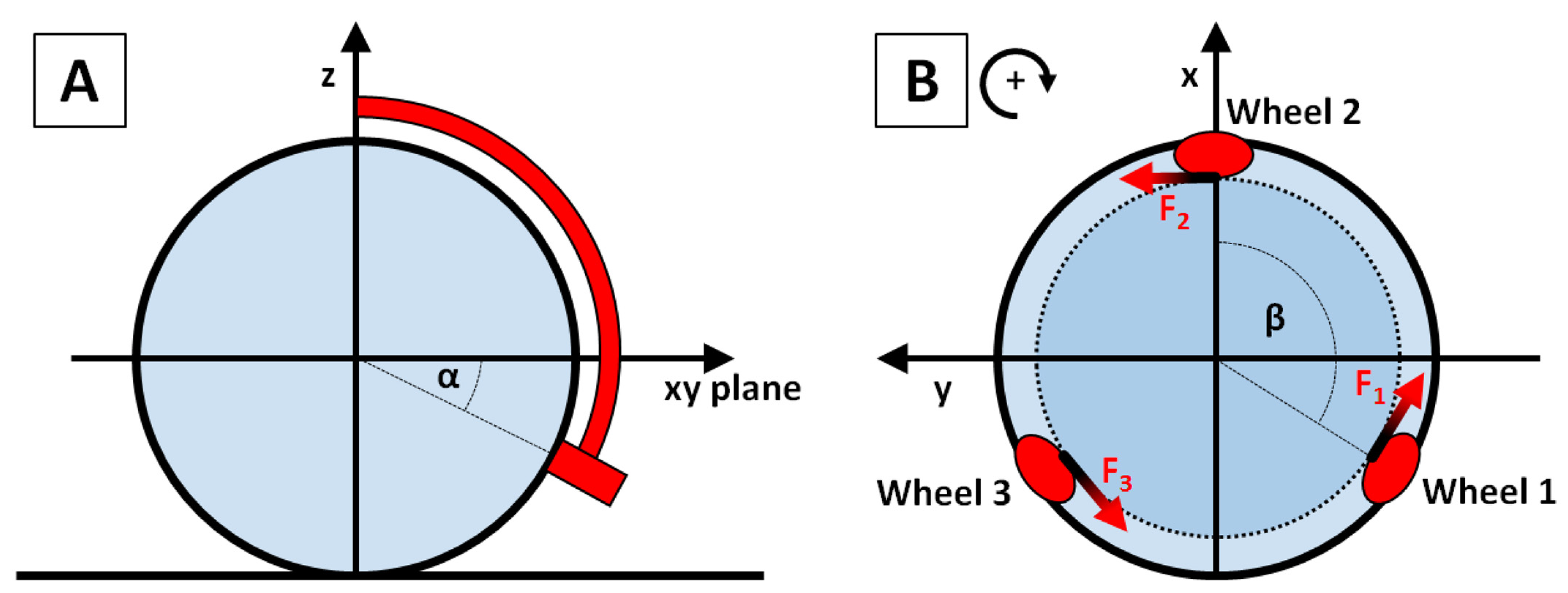
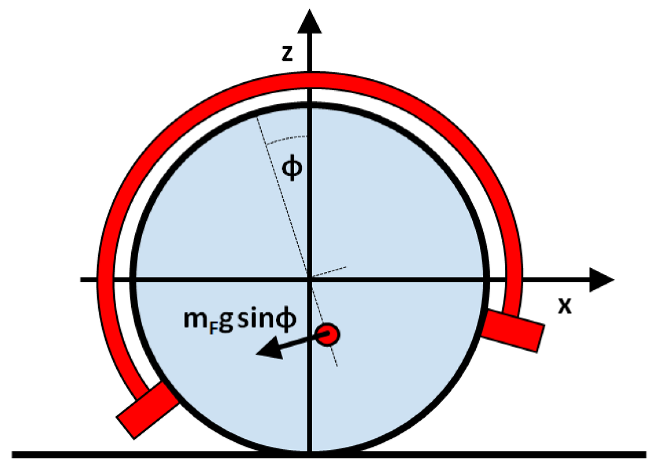
2.2. Robot Kinematics and Dynamics

To drive the robot in any of the desired motions, including translating forwards and sideways ( x ˙ ,   y ˙ ) or rotating in place ( ψ ˙ ), the tangential velocity of each of the omnidirectional drive wheels must equal the tangential velocity of the ball at the contact point. This leads to the kinematic equation for the robot (further details given in Appendix A) of
ω 1 ω 2 ω 3 = sin α 1 cos β 1 + cos β 1 r o sin β 1 sin α 1 sin β 1 + sin β 1 r o cos β 1 r cos α r o sin α 1 cos β 2 + cos β 2 r o sin β 2 sin α 1 sin β 2 + sin β 2 r o cos β 2 r cos α r o sin α 1 cos β 3 + cos β 3 r o sin β 3 sin α 1 sin β 3 + sin β 3 r o cos β 3 r cos α r o   x ˙ y ˙ ψ ˙
where ω is the wheel angular speed, r is the ball radius, ro is the driving wheel radius, α and β are subtending angles determining the height and circumferential positions of each wheel with Subscripts 1, 2, 3 corresponding to the parameters for each of the three wheels.
The reaction of the robot frame during the acceleration phase of this motion may be analysed by considering the contact forces between the wheels and the ball (details given in Appendix A). Acceleration in the x and y direction leads to a pitching and rolling, respectively, of the robot frame about the ball, which, for a small angle approximation, leads to the proportional relationship
x ¨ r d C M m F g I ϕ ,
y ¨ r d C M m F g I θ
where I is the moment of inertia of the ball, r is the ball radius, mF is the mass of the frame, dCM is the offset from the ball centre of the centre of mass of the frame with θ, ϕ being the pitch and roll angles for the robot, respectively. Acceleration in the x and y directions causes the tilting (rolling and pitching) of the robot and so the maximum acceleration possible is limited by the frame contacting the ground. To reduce this tilt, and therefore, increase the maximum possible acceleration, the centre of mass should be designed to be as low as possible (namely maximize parameter dCM).

2.3. Acceleration Control Algorithm

Due to the pendulum-like operational principle of the robot, it was anticipated that the oscillations of pitch and roll would be a significant factor during the motion of this robot. Therefore, a closed-loop control algorithm is needed to reduce the effect of these oscillations. Effectively, the pitch and roll angles need to be controlled to precise values, these being zero during constant velocity and, as seen by Equations (2) and (3), a non-zero value the during acceleration phases.
Initially, the robot controller was modelled as a positional PID algorithm but due to problems with windup, as shown by Han et al. [22] in their ballbot controller, this was changed to the velocity PID form
x ˙ = x ˙ t 1 + K P ϕ e t ϕ e t 1 + K I ϕ e t t + K D ϕ e t 2 ϕ e t 1 + ϕ e t 2 t ,
y ˙ = y ˙ t 1 + K P θ e t θ e t 1 + K I θ e t t + K D θ e t 2 θ e t 1 + θ e t 2 t .
The corresponding error terms in pitch and roll were fed into Equations (4) and (5), the outputs of which were the new translational velocities of the robot so that the resulting accelerations would result in the required tilt angles. The yaw, ψ, was simply controlled by inputting a constant value of Ψ 0, this being the maximum turning speed of the robot, to keep the frame facing in the required heading
Ψ ˙ = Ψ 0 ˙ f o r   Ψ a c t u a l < Ψ t a r g e t 0 f o r   Ψ a c t u a l = Ψ t a r g e t Ψ 0 ˙ f o r   Ψ a c t u a l > Ψ t a r g e t .
The values from (4)–(6) are substituted into Equation (1) to calculate the required angular velocities of the omni-drive wheels to correct the deviations from the desired roll, pitch and yaw. The gain parameters were tuned using the Ziegler–Nichols method.
In practice, energy losses due to friction and drag will constantly slow down the robot, and so it is expected that to maintain a constant velocity, the robot frame will need to tilt to provide a constant driving force to overcome these losses.

3. Webots Simulation

Prior to building the actual robot, a simulation of the robot using the Cybertronics open-source software Webots was developed to gain an idea of the controls needed to move the robot. A simplified model of the actual design was made on Webots, which included six omnidirectional wheels, three of which drive the robot and the other three provide passive supports at the top of the robot’s frame. The size of the robot, wheels, and ball were set to the dimensions of the real design. The main difference between the simulation and the actual robot is that the simulation uses a rigid sphere, whereas the manufactured robot utilises a compressible exercise ball made out of PVC, which results in increased friction between the ball and ground due to the larger contact area. To mitigate this effect to some extent in the simulation, the robot frame mass was set to 1 kg and the ball mass to 10 kg, thereby resulting in the preferential movement of the frame compared to the ball (as is the case in a high friction ground/ball contact). In practice, frame mass was heavier than the ball mass. The ball damping node was set to a linear and angular value of 0.2 and a basic time step of 16 ms was used for the simulations.

3.1. Building the Simulation

A simplified frame of the robot was designed on Autodesk Inventor software and imported into Webots. The omnidirectional wheels were created directly on the Webots platform. The drive wheels consist of one cylindrical hinge-joint with a rotational motor to power the wheel and 16 sub-hinge-joints with passive rollers that rotate about the axis perpendicular to the motor rotation. The wheel speeds were limited to a maximum speed of 1 rad/s to replicate actual motor performance. The passive support wheels consist of one passive cylindrical hinge-joint and eight passive rollers in the perpendicular axis. The centre of mass of the robot was translated, based on the anticipated final cad design, by 0.08 m downwards. Damping effects were added in the physics node to simulate air resistance on any oscillations. The ball was placed inside the frame, as a separate solid node independent of the robot frame. An image of the robot in this Webots simulation is shown in Figure 2. The inertial unit node in Webots was used to determine the pitch, roll and yaw angles of the robot. Due to the geometry of the frame, at a drive wheel position, the maximum tilt is 10° before frame comes in contact with the ground, whereas at midpoints between the drive wheels, the maximum tilt is 17°.

3.2. Testing in Webots

3.2.1. Open-Loop Control

To demonstrate the static stability of this concept design, the first test conducted was to observe the response of the robot with the frame tilted at −9° in the roll axis and +3° in the pitch axis whilst the motors were not powered. The IMU angles were recorded over a 26 s simulation time. The results are shown in Figure 3. Note that there are no horizontal translations of the ball, just pitch and roll rotations. Due to the simulated air effects, the oscillations were slowly dampened.
The second test conducted was driving the robot forwards with open-loop control to observe the oscillations in the roll, pitch and yaw. To steer the robot in any direction, the linear velocities in x and y and the yaw speeds are input into Equation (1) to determine the required motor velocities. For this test, the robot was translated at 0.05 m/s, and then at 0.1 m/s along the x axis, while the y velocity and yaw speed were set to 0. Figure 4 shows the results for the roll, pitch and yaw angles.
As the robot accelerates, a tilt opposite the direction of travel is expected due to the conservation of angular momentum between the robot frame and the ball, subsequently followed by oscillations similar to the static case. At a velocity of 0.05 m/s, the pitch of the robot reaches an initial angle of −8.3° before going into oscillation, with the roll and yaw angles being maintained at 0°. At 1 m/s, the initial angle doubles to −16.6°, with the subsequent oscillation at the 5.0 s time point causing the robot frame to collide with the ground. This resulted in oscillations of ±0.2° in the roll and a linear increase in the yaw from 0° to 4° causing the robot to go off path. A lower centre of mass would reduce oscillation amplitude; however, there will always be an acceleration limitation in the open-loop configuration due to this effect.

3.2.2. Closed-Loop Control

For the closed-loop control strategy, a target roll, pitch, and yaw were set. The measurements of the current angle from the IMU were then used to determine the error in position. These values are used in Equations (4) and (5) to determine the required velocities to correct for this error. For PID-tuning, the error terms were plotted in Webots against simulation time and the Ziegler–Nichols method used to determine values 10, 4 and 0.05 for proportional, integral and differential gain terms, respectively. These values showed consistent convergence to dampen the error to small oscillations of less than 0.1°. It was anticipated that retuning would be required on the actual robot.
The first test for the closed-loop control was to repeat the static (no robot translation) test. The robot was tilted to −9° and +3° degrees at 2 s about the roll and pitch axis, respectively, and then the PID controller was implemented at 2.7 s with a target angle of 0° set on all three axes. Results are shown in Figure 5. The controller completely dampens the oscillations and within 9 s of the disturbance, the target position is achieved and maintained to ±0.1° degrees about all three axes.
The second and third tests were to translate the robot using the PID controller by setting a non-zero pitch and roll angles to move the robot towards an arbitrarily chosen heading of −135°. For the second test, an initial disturbance in pitch and roll of −3.5° and 6.1°, respectively, at 2.5 s were applied to the robot. Then, at 3.1 s the PID was implemented to translate the robot without rotating, namely keeping the same heading for the front of the robot. Thus, target rotations of [+1, −1, 0] corresponding to the required pitch, roll and yaw angles were fed into the PID controller. The results are given in Figure 6, where the robot is shown to move straight at −135°. Small oscillations of 0.03° are visible whilst the yaw of the robot is maintained at 0.
Due to how the camera sensor is mounted on the robot, there is the scenario that the robot has a preferred front direction. Therefore, the third test involved translating the robot at a −135° heading whilst keeping the robot orientation fixed towards the direction of travel. To simulate this direction of motion, the robot can either turn in place to −135° and then go straight or move forwards and steer simultaneously where the radius of curvature of the path is a function of the ratio between translation and rotational velocities. The latter was chosen as the test scenario. Target angles of [−2, 0, −135] were fed in the PID controller, the results are shown in Figure 7. The plot shows the initial convergence of the roll and pitch angles to their target values of 0 and −2 while the robot steers to the target yaw. While the robot rotates, oscillations of ±0.15° are seen in the pitch and roll angles. When the robot reaches the target yaw of −135° at 31.2 s, the instantaneous rate of change of angular rotation causes a spike in the pitch and roll of magnitude 0.5°. However, within 5 s, this is corrected back to the target values.
The simulations demonstrate the feasibility of the robot design and suitable options for its control. The next stage was to create a physical realization of this design.

4. Prototype

4.1. Mechanical Build

The aim for the mechanical build of the robot was to produce a rigid frame, to encompass an inflatable ball, with its centre of mass located below the centre of the ball whilst achieving sufficient ground clearance. This prototype was constructed from 6mm plywood, an exploded CAD image of the frame design is shown in Figure 8. The main features of this design are:
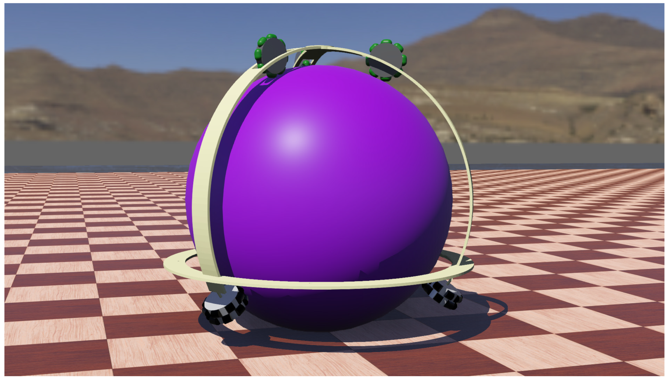
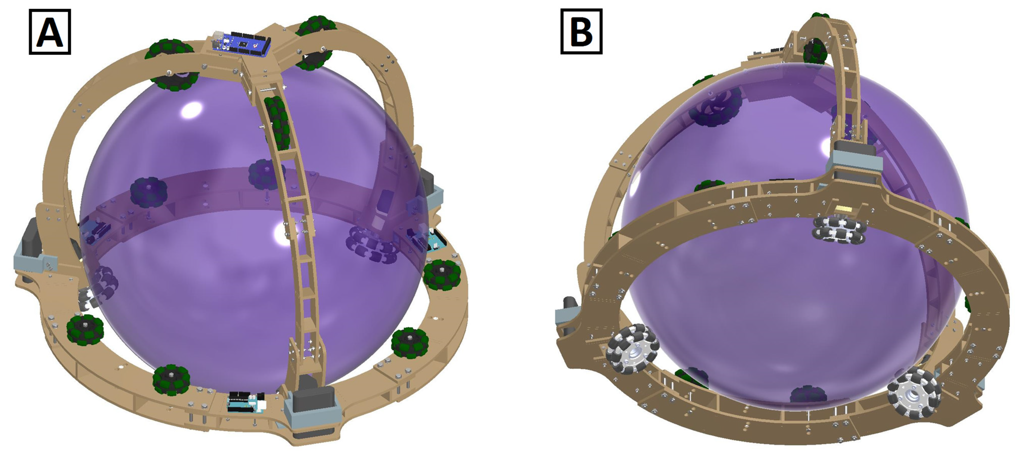
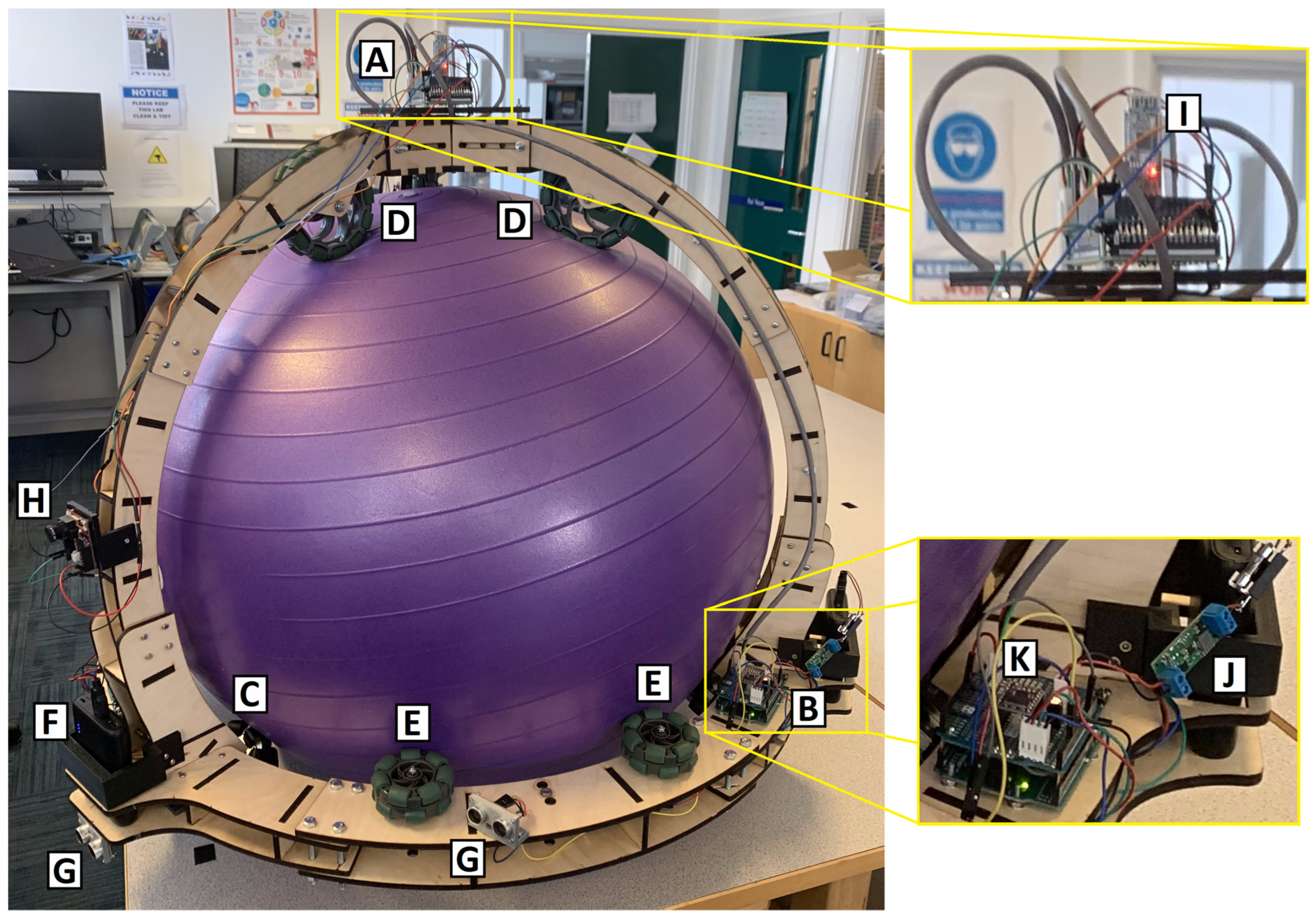
  • A halo located around the lower hemisphere of the ball. The purpose of the halo ring is to provide a mounting point for the drive wheels whilst lowering the centre of mass of the robot. The halo was made in two layers, this provided for a more rigid structure and increased the amount of weight below the centre of the ball. The use of additional bolts on the halo allowed for the adjustment of the weight and centre of mass of the robot. The double-layered design also made cable management much simpler as the wires were secured, routed within the layers. In addition, the halo served as a bumper for the robot;
  • Supporting arms, attached to a top mounting plate, supported the halo in the correct position. Similar to the halo, these were made in two layers. It was important to optimise the mass of this part of the structure as its location high on the robot significantly affects the position of the overall centre of mass.
  • Three symmetrically placed driven omnidirectional wheels. Due to the weight of the corresponding motors and batteries, these are placed on the halo to help maintain an overall low centre of mass;
  • Three passive omnidirectional wheels placed on the supporting arms ensured that the drive wheels maintained contact with the ball;
  • Three 27:1 planetary geared stepper motors (Stepperonline, 17HS13-0404S-PG27) were used to drive the robot. Each of these 12V motors had a maximum permissible torque of 3 Nm and maximum speed of 9 rpm. The motor speed was limited to their start/stop range, and motor velocity control was operated in an open-loop configuration.
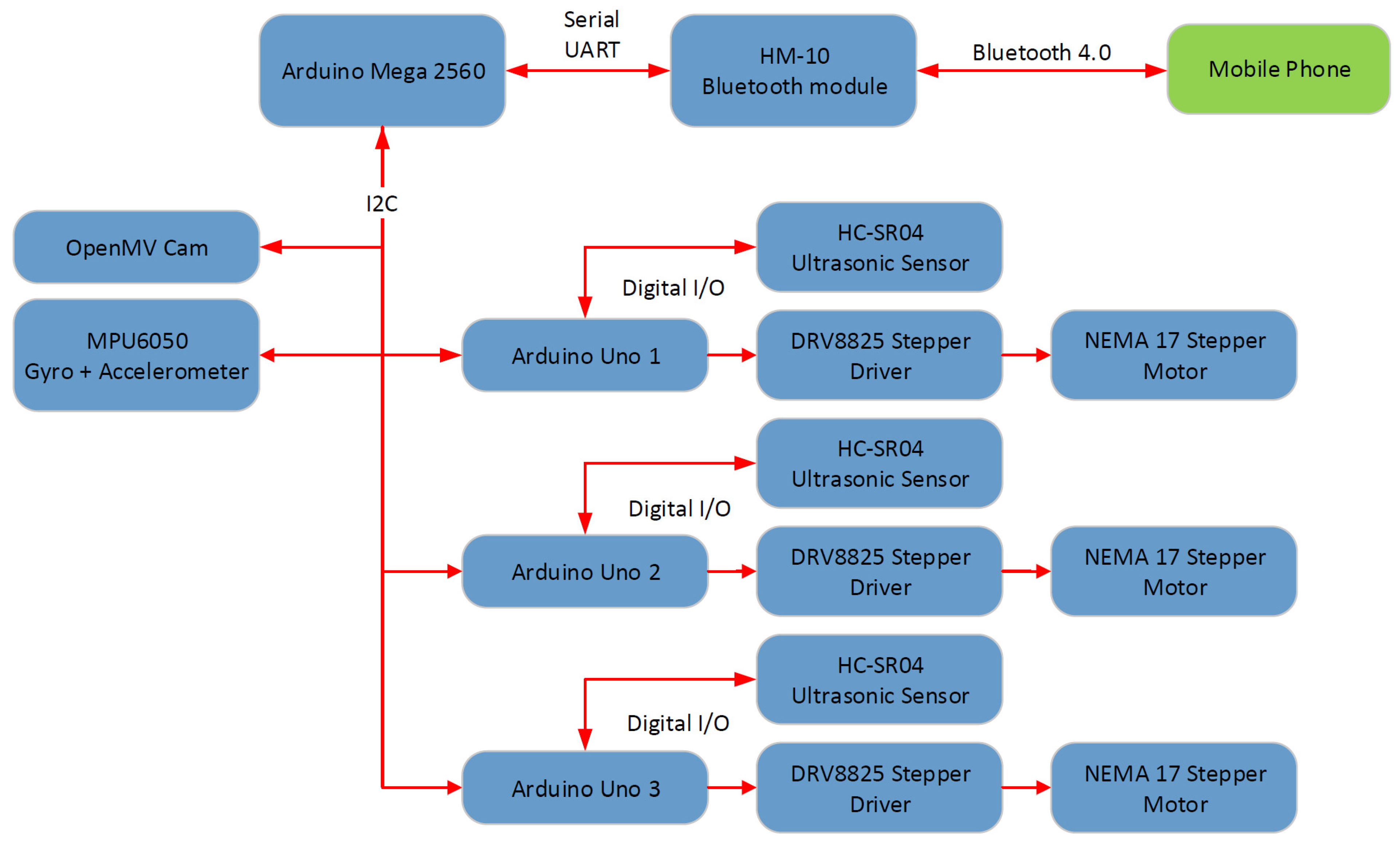
4.2. Electronics

A schematic of the electronics and communications configuration is shown in Figure 9. The main features of this arrangement are:
  • A primary Arduino located in the top housing of the robot provides the control commands and communications interface;
  • Three secondary Arduinos are used to control each motor through a Popolu DRV8825 driver chip. They are connected to the primary Arduino via I2C communications and positioned close to their respective motors;
  • Three Anker 5 V, 10,400 mAH power banks (one for each motor) supplies the required current to the motors and corresponding drive electronics. These were attached close to the motors using custom 3D printed housing. The Arduino and sensors are directly connected to the power banks; the motors are connected via a Popolu 12V step-up voltage regulator (U3V70F12). The primary Arduino is powered from one of these power banks;
  • A six-degree-of-freedom MPU6050 motion-tracking device, containing an accelerometer and gyroscope, is utilised to measure roll, pitch, and yaw values. This IMU is located in the top housing, vertically aligned with the centre of mass and connected to the primary Arduino;
  • A HM-10 Bluetooth module provides the option to remotely control the robot. The Dabble smartphone app was used as the user interface for this option;
  • Additional sensors included an array of HC-SR04 ultrasonic sensors and an OpenMV camera. Although not reported here, the intention is to utilise these sensors towards the future autonomous control of the robot.

4.3. Final Adjustments

For this prototype, the frame design was rigid with no suspension provided at the contact points with the ball; as it was anticipated, flexibility in the inflatable ball would provide this aspect. During testing, issues with offsets in the ball’s position within the frame resulted in additional passive omnidirectional wheels being placed around the halo to help centralize the ball within the frame structure, the positions of these additional wheels are shown in Figure 8.
For the final constructed prototype, the mass of the frame was 9.19 kg with the motors, wheels and power banks accounting for 4.35 kg of this mass. Ball mass was 1.4 kg. The position of the centre of mass of the frame was 79.2 mm below the centre of the ball. An image of the finally constructed robot is shown in Figure 10.

4.4. Testing

The robot was first tested for static stability. Figure 11 shows the response of the robot when stationary but with an induced disturbance. Initially, a pitch angle of approximately 7° is exerted on the robot followed by a 8.5° tilt in roll 20 s later. In this open-loop configuration, oscillations were damped to within 0.5° within 15 s and 30 s, respectively similar to that shown in the simulation. Some coupling of the motion into the other axes can be seen, as yaw is small; then, this is attributed to asymmetries in the centring of the frame about the ball rather than any Coriolis effects.
The robot is designed to move with three degrees of freedom, including translation along the pitch and roll axes and rotations in yaw. Figure 12 demonstrates the robot’s response to be driven at 0.05 m/s in the x direction, and then rotating the robot on the spot, both in open-loop configuration. As seen in the simulation, when translated in the x direction, oscillations are seen in the pitch angle around a 5° offset. A coupling of this oscillation is seen in the roll angle and some yaw is introduced. For the rotation on the spot, displacements and subsequent oscillations are seen in both pitch and roll angles as the yaw rate is changed from 0 rad/s through 0.5 rad/s, 1 rad/s and finally to −1 rad/s.

4.5. Discussion

4.5.1. Current Issues

The physical robot showed similar characteristics to the simulation during motion, demonstrating the basic feasibility of the concept. However, the main difference to the simulation was the characteristics of the ball used, which had a significant impact on the performance of the actual robot; it was not possible to simulate ball compressibility in the Webots model.
The robot frame was designed for a 65 cm diameter inflatable exercise ball, with some room for adjustment incorporated into the design of the frame. The simulation utilised a solid 65 cm diameter incompressible sphere. On assembly of the robot, it was found that for the current design, the amount of inflation of the ball was critical to obtaining an optimised performance. For the recommended inflation, there was too much compliance in the ball resulting in pressure from the omni wheels causing an indentation of the ball at the point of contact, the robot making a flat contact point with the ground and the ball shifting from a central position and contacting the frame during motion. The addition of the extra omni wheels on the halo partially, although not completely, rectified this latter problem. Increasing the pressure within the ball, thereby making the ball less compressible, reduced the indentation and ground contact issues; however, the enlarged ball size then made frame-contacting more of a problem. Thus, for this prototype design a compromise on ball inflation was used. Due to these issues, the PID algorithms to control the tilt angle developed in the simulation stage could not be successfully demonstrated with this prototype.
A second issue found with the current robot design was that the motors could not provide enough torque to fully test the robot capabilities. In principle, such a ball robot should be able to navigate step changes in ground level and also have the ability to traverse gradients. Inclines of up to 3° were successfully navigated but beyond this and for step changes, there was insufficient torque provided by the motors. Ultimately, step and gradient limits will be defined by the radius of the ball and the position of the halo.

4.5.2. Future Developments

The main development need is the ball itself. An inflatable ball provides an easy purchase and assembly, as the ball can be inflated inside the robot frame; however it, may have to be inflated above the recommended pressure to minimise compressibility. An inflatable ball also offers the ability to tune the ball pressure to optimise the robot performance in terms of terrain compliance. The development of a suitable analytical model or simulation to replicate the compressibility characteristics of such a ball would be required for such developmental work, possibly by using a viscoelastic model, as described by Goodwill et al. [23]. Ribbing may also be an issue with this option. Buying or manufacturing a rigid hollow sphere is an alternative option, although weight, strength and symmetry may be issues to contend with. In either case, the frame design needs tight tolerances on its manufacture or the ability to adjust to accommodate the precise positioning of the ball within the frame. More powerful motors for this size of robot were identified as a requirement whilst in addition providing suspension on the omni wheels would help to maintain a constant contact force between the drive wheels and the ball, thereby allowing for a more predictable control of the robot. The above improvements would see a vast improvement in the performance of the prototype robot.
The actual position of the centre of mass of the robot with respect to the ball position then becomes the main target of optimisation. The current design allows masses of up to 1.7 kg located on the top platform whilst still allowing for static stability with larger masses possible if placed lower on the frame. This limit may be further improved either by lowering the original centre of mass or increasing the mass of the frame. Increasing the mass is the simplest solution to implement but comes at the expense of either performance (by adding deadweight to the halo) or cost (by increasing the size of the motors). Lowering the centre of mass position improves static stability, thereby increases the statically stable load-bearing capacity, reduces oscillations seen during motion and allows for greater accelerations, whereas raising this towards the centre of the ball improves both ground clearance and its ability for gradient and step change traversals.

5. Conclusions

Due to their single-point contact, ball robots offer an omnidirectional motion over non uniform terrain; however, their main drawback is that they must be continually powered to maintain dynamic stability. The work reported here has demonstrated the successful development of a novel statically stable and omnidirectional ball robot in which the robot is stable when both powered and unpowered due to its low centre of mass. A computer simulation of the design showed very promising results in the manoeuvrability and control of the robot using a PID algorithm. The constructed prototype did highlight some manufacturing issues but, for this first attempt, did demonstrate static stability and three degrees of freedom functionality with a maximum operation linear speed of 0.05 m/s, rotation angular speed of 1 rad/s and the ability to traverse an incline of 3°.
Although this robot design is not suited to the tall slender aspect ratios of traditional balancing ballbots, which are ideal for human interaction, the Stastaball design has the flexibility for a number of applications, including load-carrying. Currently Stastaball is capable of carrying up to 1.7 kg whilst remaining statically stable. For such load-bearing scenarios in which the position of the centre of mass varies either below or possibly above the centre of the ball depending on the load, H or µ control methods would be needed to optimise the controller to account for such a variation or an adaptive dynamic controller developed tuned for various load-bearing scenarios. For a collaborative load-carrying, either between robot–robot interaction or human–robot interaction, as demonstrated by Kugle [24], the planar constraint at the load interface helps provide the stabilization needed. In addition to load-carrying, other potential applications for such robots include exploration, surveillance and their use as education platforms.
The Stastaball concept allows for static stability compared with ball-balancing and unicycle robots, omnidirectional motion compared to monocycle designs and options for mechanical interactions as compared to robots contained within spheres. Future work on addressing the advantages and complexities of ball compressibility, centre of mass positioning and appropriate controller development opens up new lines of research into the application of such a robot concept into real world applications.

Author Contributions

Conceptualization, J.H.; methodology, L.F., J.Y., T.M. and E.K.; software, L.F.; validation, L.F., J.Y., T.M. and E.K.; investigation, L.F., J.Y., T.M. and E.K.; writing—original draft preparation, L.F., J.Y., T.M. and E.K.; writing—review and editing, J.H.; project administration, J.H. All authors have read and agreed to the published version of the manuscript.

Funding

This research received no external funding.

Data Availability Statement

The data presented in this study are openly available in data.ncl at https://doi.org/10.25405/data.ncl.21977720 (accessed on 20 February 2023).

Acknowledgments

The authors wish to acknowledge Paul Watson, Paul Harrison and Frank Atkinson for technical assistance during construction of the robot.

Conflicts of Interest

The authors declare no conflict of interest.

Appendix A

To move the robot, three drive wheels tangential to the surface of the ball produce a force that generates the rolling motion of the ball. As a result, the entire robot can move with three degrees of freedom: translations along x and y directions and rotation about z.
Consider one of the driven omnidirectional wheels applying a force on the ball. The wheel is positioned to apply a force on the ball in a direction parallel to the ground plane. Given a Cartesian coordinate system (x, y and z), the contact point of this force in polar coordinartes is (r, α and β) where r is the radius of the ball, α is the subtending angle from the xy plane and β is the angular position about the z axis with respect to the x axis direction. This is shown in Figure A1. For motion in the x direction, the ball must rotate about the y axis, for motion in the y direction, the ball must rotate about the x axis, whilst for turning, the ball must spin about the z axis.
Figure A1. (A) Side view of the robot showing placement of one of the drive wheels. (B) Top view of the robot showing placement of the three drive wheels. The force imparted on the ball by the wheels, shown by the arrows, results in the frame rotating in the opposite direction (clockwise for the case shown).
Robotics 12 00034 g0a1
For the geometry shown in Figure A1, the sum of the moments about the y axis produced by the motors is:
M y _ M = r sin α n = 1 3 F n sin β n
where r is the ball radius and the subscripts denote the parameter with respect to wheels 1, 2 and 3. This produces an angular acceleration of the ball, ϕ ¨ , about the y axis and a resulting translational acceleration, x ¨ , (due to rolling) in the x direction:
M y _ M = I ϕ ¨ = I x ¨ r
where I is the moment of inertia of the ball about the x (and y, z) axis. The sum of the moments applied to the ball result in an equal and opposite moment being applied to the frame. This moment tilts the frame and forces the centre of mass of the frame, mF, offset from the centre of the ball by a distance of dCM, away from the z axis, as shown in Figure A2.
Figure A2. The moment produced by the driving wheels results in a tilting of the frame, which is then balanced by the moment produced from the gravitational force on the offset centre of mass.
Robotics 12 00034 g0a2
The gravitational restoring force for this offset centre of mass results in a moment about the y axis of:
M y _ G = d C M m F g sin ϕ
The sum of all these moments about the y balance give, from Equations (A2) and (A3):
I x ¨ r + d C M m F g sin ϕ = 0
x ¨ = r d C M m F g I sin ϕ
which for small pitch angles approximates:
x ¨ r d C M m F g I ϕ
Alternatively, in terms of force, Equations (A1) and (A3) give
r sin α n = 1 3 F n sin β n + d C M m F g sin ϕ = 0
sin ϕ = r sin α d C M m F g n = 1 3 F n sin β n
which for small pitch angles approximates:
ϕ r sin α d C M m F g n = 1 3 F n sin β n
A similar argument is made for moments about the x axis leading to a translational velocity of the robot in the y direction. In this case, all three driving wheels contribute to the driving force leading to equations:
y ¨ r d C M m F g I θ ,
θ r sin α d C M m F g n = 1 3 F n cos β n .
All three driving wheels also contribute to the rotation, or yaw, of the robot, ψ . In this case, as the drive is symmetric about the z axis, there is no resulting tilt on the robot. The sum of moments leads to an indistinguishable turning of the ball and a noticeable rotation of the frame given by:
M z = r sin α n = 1 3 F n = I ψ ¨ ψ ¨ = r sin α I n = 1 3 F n
Once the desired speed is achieved, the tangential speed of the driving omni wheels matches the tangential speed of the ball and a force is no longer being applied. The tilting of the frame will, therefore, return to zero and remain at this whilst the velocity is constant and acceleration is not required. The problem now simplifies to a kinematic analysis in which the speed of the omni wheels is constrained to match the speed of the contact point of the surface as demonstrated by Siegwart [25] for a ground contact. In this case, we consider wheel contact with the surface of the ball, as shown in Figure A1.
For a ground speed of x ˙ then the surface velocity at the omni wheel/ball contact point, vc, can vary from x ˙ sin α when the wheel is located furthest from the x axis (when β is ±90°) to x ˙ when the wheel is located on the x axis (when β is 0° or 180°). The surface contact point velocity is thus:
v c = x ˙ sin α + cos β x ˙ x ˙ sin α
Rearranging gives:
v c = x ˙ sin α 1 cos β + cos β
The component of translational velocity in the x direction for the omni wheel, which for no slip must equal vc, is:
v c = r o ω sin β
where ro is the omnidirectional wheel radius and ω is the wheel angular velocity. Equating Equations (A9) and (A10) gives:
x ˙ sin α 1 cos β + cos β = r o ω sin β
For the undefined case of β is 0° or 180°, the wheel is perpendicular to the direction of travel, and therefore, uses its rollers to free wheel in this direction.
Similarly by considering a ground speed of y ˙ gives:
y ˙ sin α 1 sin β + sin β = r o ω cos β
and ψ ˙ :
ψ ˙ r cos α = r o ω
Rearranging Equations (A11)–(A13) and putting in matrix form for all the three omni wheels gives
ω 1 ω 2 ω 3 = sin α 1 cos β 1 + cos β 1 r o sin β 1 sin α 1 sin β 1 + sin β 1 r o cos β 1 r cos α r o sin α 1 cos β 2 + cos β 2 r o sin β 2 sin α 1 sin β 2 + sin β 2 r o cos β 2 r cos α r o sin α 1 cos β 3 + cos β 3 r o sin β 3 sin α 1 sin β 3 + sin β 3 r o cos β 3 r cos α r o   x ˙ y ˙ ψ ˙
For open-loop control, the required x ˙ , y ˙ and ψ ˙ values are set and from (A14), the appropriate motor speeds are determined. The force resulting from the mismatch in speeds between the omni wheels and the ball during the acceleration phase will result in a tilting of the robot, as given by (A5) and (A7). For closed-loop control, the tilt angles are controlled.

References

  1. Lauwers, T.; Kantor, G.; Hollis, R. One is enough! In Proceedings of the International Symposium for Robotics Research, San Francisco, CA, USA, 12–15 October 2005; pp. 327–336. [Google Scholar]
  2. Shut, R.; Hollis, R. Development of a Humanoid Dual Arm System for a Single Spherical Wheeled Balancing Mobile Robot. In Proceedings of the 2019 IEEE-RAS 19th International Conference on Humanoid Robots (Humanoids), Toronto, ON, Canada, 15–17 October 2019; pp. 499–504. [Google Scholar] [CrossRef]
  3. Kumagai, M.; Ochiai, T. Development of a Robot Balanced on a Ball—First Report, Implementation of the Robot and Basic Control. J. Robot. Mechatron. 2010, 22, 348–355. [Google Scholar] [CrossRef]
  4. Fankhauser, P.; Gwerder, C. Modeling and Control of a Ballbot. Bachelor’s Thesis, Swiss Federal Institute of Technology, Zurich, Switzerland, 2010. [Google Scholar]
  5. Jespersen, T.K. Kugle—Modelling and Control of a Ball-Balancing Robot. Master’s Thesis, Aalborg University, Aalborg, Denmark, April 2019. [Google Scholar]
  6. Gao, X.; Yan, L.; He, Z.; Wang, G.; Chen, I.-M. Design and Modeling of a Dual-Ball Self-Balancing Robot. IEEE Robot. Autom. Lett. 2022, 7, 12491–12498. [Google Scholar] [CrossRef]
  7. FESTO. Available online: https://www.festo.com/gb/en/e/about-festo/research-and-development/bionic-learning-network/highlights-from-2018-to-2021/bionicmobileassistant-id_326923/ (accessed on 20 February 2023).
  8. Nagarajan, U.; Kantor, G.; Hollis, R. The ballbot: An omnidirectional balancing mobile robot. Int. J. Rob. Res. 2014, 33, 917–930. [Google Scholar] [CrossRef]
  9. Nagarajan, U.; Hollis, R. Shape space planner for shape-accelerated balancing mobile robots. Int. J. Rob. Res. 2013, 32, 1323–1341. [Google Scholar] [CrossRef] [Green Version]
  10. Hertig, L.; Schindler, D.; Bloesch, M.; Remy, C.; Siegwart, R. Unified state estimation for a ballbot. In Proceedings of the 2013 IEEE International Conference on Robotics and Automation, Karlsruhe, Germany, 6–10 May 2013; pp. 2471–2476. [Google Scholar] [CrossRef]
  11. Jespersen, T.K.; Ahdab, M.A.; Méndez, J.D.D.F.; Damgaard, M.R.; Hansen, K.D.; Pedersen, R.; Bak, T. Path-Following Model Predictive Control of Ballbots. In Proceedings of the 2020 IEEE International Conference on Robotics and Automation (ICRA), Paris, France, 31 May–31 August 2020; pp. 1498–1504. [Google Scholar] [CrossRef]
  12. Zhou, Y.; Lin, J.; Wang, S.; Zhang, C. Learning Ball-Balancing Robot through Deep Reinforcement Learning. In Proceedings of the 2021 International Conference on Computer, Control and Robotics (ICCCR), Shanghai, China, 8–10 January 2021; pp. 1–8. [Google Scholar] [CrossRef]
  13. DIY Sphere Robot. Available online: https://www.instructables.com/DIY-Sphere-Robot (accessed on 20 February 2023).
  14. Sphero. Available online: https://sphero.com/products/sphero-bolt (accessed on 20 February 2023).
  15. Chase, R.; Pandya, A. A Review of Active Mechanical Driving Principles of Spherical Robots. Robotics 2012, 1, 3–23. [Google Scholar] [CrossRef]
  16. Tholapu, S.; Sudheer, A.P.; Joy, M.L. Kinematic Modelling and Structural Analysis of a Spherical Robot: BALL-E. IOP Conf. Ser. Mater. Sci. Eng. 2021, 1132, 012034. [Google Scholar] [CrossRef]
  17. Cardini, S.B. A history of the monocycle stability and control from inside the wheel. IEEE Control. Syst. Mag. 2006, 26, 22–26. [Google Scholar] [CrossRef]
  18. Cieslak, P.; Buratowski, T.; Uhl, T.; Giergiel, M. The mono-wheel robot with dynamic stabilisation. Rob. Auton. Syst. 2011, 59, 611–619. [Google Scholar] [CrossRef]
  19. Geist, A.R.; Fiene, J.; Tashiro, N.; Jia, Z.; Trimpe, S. The Wheelbot: A Jumping Reaction Wheel Unicycle. IEEE Robot. Autom. Lett. 2022, 7, 9683–9690. [Google Scholar] [CrossRef]
  20. Shen, J.; Hong, D. OmBURo: A Novel Unicycle Robot with Active Omnidirectional Wheel. In Proceedings of the 2020 IEEE International Conference on Robotics and Automation (ICRA), Paris, France, 31 May–31 August 2020; pp. 8237–8243. [Google Scholar] [CrossRef]
  21. Cai, C.; Lu, J.; Li, Z. Kinematic Analysis and Control Algorithm for the Ballbot. IEEE Access 2019, 7, 38314–38321. [Google Scholar] [CrossRef]
  22. Han, H.Y.; Han, T.Y.; Jo, H.S. Development of omnidirectional self-balancing robot. In Proceedings of the 2014 IEEE International Symposium on Robotics and Manufacturing Automation (ROMA), Kuala Lumpur, Malaysia, 15–16 December 2014; pp. 57–62. [Google Scholar] [CrossRef]
  23. Goodwill, S.; Haake, S. Modelling of tennis ball impacts on a rigid surface. Proc. Inst. Mech. Eng. C-J. Mech. E 2004, 218, 1139–1153. [Google Scholar] [CrossRef]
  24. IEEE Spectrum. Available online: https://spectrum.ieee.org/042910-a-robot-that-balances-on-a-ball (accessed on 20 February 2023).
  25. Siegwart, R.; Nourbakhsh, I.R. Introduction to Autonomous Mobile Robots, 1st ed.; The MIT Press: Cambridge, MA, USA, 2004; pp. 53–67. [Google Scholar]
Figure 1. The operational principle of a statically stable ball robot. As the centre of mass of the robot (CM) is lower than the centre of rotation (CR) of the ball, any induced tilt onto the robot will result in a restoring force that corrects for this tilt.
Robotics 12 00034 g001
Figure 2. The Stastaball robot as simulated in Webots. A solid sphere of mass 10 kg was used as the central ball. Frame mass was 1 kg and offset downwards from ball centre by 0.08 m.
Robotics 12 00034 g002
Figure 3. Response of the stationary robot when a pitch and roll disturbance is introduced in the first 1.3 s.
Robotics 12 00034 g003
Figure 4. Rotation of the robot frame as the robot translates in the x direction, the dotted horizontal lines show the maximum pitch angle for the robot. At 0.05 m/s (shown in (A)), oscillations are seen in the pitch angle. At 0.1 m/s (shown in (B)), the excessive pitching causes the frame to collide with the ground at 5.0 s, causing movement in the roll and yaw.
Robotics 12 00034 g004
Figure 5. Recovery of the robot to a disturbance at 2 s using a PID controller to correct frame orientation. The PID controller was activated at 2.7 s.
Robotics 12 00034 g005
Figure 6. Response of the robot to an initial disturbance at 2 s followed by a command at 3.1 s to translate towards a heading of −135° with PID implemented.
Robotics 12 00034 g006
Figure 7. Response of the robot to a command to move forward with a heading of −135° with PID implemented. Initial heading is 0°. Sudden changes in yaw causes disturbances in pitch and roll as seen at 31.2 s.
Robotics 12 00034 g007
Figure 8. CAD drawing of the robot viewed from (A) above and (B) below from where the drive wheels are clearly visible. Six omnidirectional support wheels on the halo of the robot were incorporated to help centralize the ball within the frame.
Robotics 12 00034 g008
Figure 9. Schematic of the communication structure of the robot.
Robotics 12 00034 g009
Figure 10. Image of the constructed prototype of Stastaball showing a primary Arduino (A); a secondary Arduino (B); a driven wheel (C), which is partially visible behind the halo; passive support wheels on the frame (D); and halo (E); one of the power banks (F); ultrasonic sensors (G); and camera (H). Upper inset shows zoomed view of primary Arduino containing Bluetooth module (I) and IMU module (not visible in this image). Lower inset shows zoomed view of one of the secondary Arduinos with voltage regulator (J) and motor driver (K) mounted onto an Arduino shield.
Robotics 12 00034 g010
Figure 11. Static stability test for the robot. Induced displacements in the pitch and then roll angles demonstrate damped oscillations back to the static position.
Robotics 12 00034 g011
Figure 12. Response of the robot in the pitch, roll and yaw axes when (A) being driven at 0.05 m/s in the x direction and (B) programmed to rotate on the spot at varying yaw rates.
Robotics 12 00034 g012aRobotics 12 00034 g012b
Disclaimer/Publisher’s Note: The statements, opinions and data contained in all publications are solely those of the individual author(s) and contributor(s) and not of MDPI and/or the editor(s). MDPI and/or the editor(s) disclaim responsibility for any injury to people or property resulting from any ideas, methods, instructions or products referred to in the content.

