Abstract
For autonomous legged robots to be deployed in practical scenarios, they need to perform perception, motion planning, and locomotion control. Since robots have limited computing capabilities, it is important to realize locomotion control with simple controllers that have modest calculations. The goal of this paper is to create computational simple controllers for locomotion control that can free up computational resources for more demanding computational tasks, such as perception and motion planning. The controller consists of a leg scheduler for sequencing a trot gait with a fixed step time; a reference trajectory generator for the feet in the Cartesian space, which is then mapped to the joint space using an analytical inverse; and a joint controller using a combination of feedforward torques based on static equilibrium and feedback torque. The resulting controller enables velocity command following in the forward, sideways, and turning directions. With these three velocity command following-modes, a waypoint tracking controller is developed that can track a curve in global coordinates using feedback linearization. The command following and waypoint tracking controllers are demonstrated in simulation and on hardware.
1. Introduction
For quadrupeds and legged robots to be practical in search and rescue, industrial, and home scenarios, they need to be able to follow high-level commands (e.g., moving forward and sideways as well as turning) and to perform high-fidelity tracking of waypoints for navigation in constrained environments. The availability of limited computational resources complicates on-board control. Although it is possible to add more computing resources, these would consume energy, thus, depleting the charge on the batteries.
There are two broadly used methods. One, use a model to generate controllers offline, save them on the robot hardware, and search and deploy the correct controller based on sensor data. This approach is computationally simple but may not generalize to novel scenarios that have not been tested in simulation. Two, use a numerical approach (e.g., optimization) to generate controllers on the fly. This approach generalizes to novel scenarios but is computationally more challenging.
In this paper, our goal is to create a computational simple trot controller for quadruped robots and demonstrate that it is capable of high-fidelity command following and waypoint tracking. Our trot controller relies on analytical solutions and simple matrix manipulations, thus, enabling quick computations. The controller is able to demonstrate omnidirectional walking (motion in the fore–aft, lateral, and yaw directions) and can be combined with an appropriate model for waypoint tracking (tracking a curve in horizontal space).
The paper is organized as follows. The review of related literature is found in Section 2. The low-level and high-level controllers are presented in Section 3 and Section 4, respectively. The simulation and hardware results are presented in Section 5, followed by the discussion in Section 6, and our conclusions and future work in Section 7.
2. Background and Related Work
One of the first papers on the dynamic movement of quadruped robots considered multi-leg control by extending the controller developed for balancing on one leg [1]. The controller comprises three decoupled modes with each one regulating a different aspect of the balance: (1) a foot-placement control in the flight phase for regulating the speed, (2) thrust in the telescopic leg during the stance phase for regulating the height, and (3) torque between the leg and body during the stance phase for regulating the torso attitude. When this one-legged controller is properly deployed between the four legs, it is possible to generate a trot, pace, and bounding gait. Other have extended these simple heuristics for galloping and bounding gaits [2].
There are various other heuristic approaches that have led to successful locomotion control. In virtual model control, the movement of the body is planned using virtual components, such as springs and dashpots [3]. The resulting forces in Cartesian coordinates are converted to joint torques using the Jacobian of the foot with respect to the joint angle [4]. In central pattern generators, neural networks are used to represent the control policy. The weights of the neural network are then tuned on the system in simulation and hardware to generate various gaits [5,6].
Model-based control approaches for locomotion are based on a simple reduced order model of the system. These models have, as its inputs, the ground reaction forces on the stance legs and foot placement in the swing phase. The ground reaction forces are computed to ensure periodicity [7] or are based on solving a model predictive controller to track a prescribed reference motion [8,9]. They, then, implement the resulting ground reaction force profiles and foot placement on the robot using a combination of feedforward and feedback torques.
The quality of the solution depends on the model simplification used. A simple approach is to linearize the dynamics and use automatic differentiator, such as CasADi, to compute the gradients [10]. Better approaches to linearization using exponential coordinates allow for a better approximation of the linearized dynamics [11]. Another approach is to use full nonlinear dynamics for control but use computationally simple approximations of the derivatives [12]. By adding an event-based model predictive controller, the controller is able to better handle friction constraints [13].
Model-free methods for locomotion are based on reinforcement learning. The goal is to train a neural network that takes in, as inputs, the position and velocity of the legs and torso and returns outputs of either the joint torques [14] or joint reference angles [15]. However, reinforcement learning is not sample efficient. To overcome this, one can seed the learning with samples from a motion-capture system [16] or learn in a lower-dimensional space, such as in the Cartesian space [17].
Another issue with such approaches is that policies learned in simulation do not transfer well to hardware. This is known as the reality gap. To narrow the reality gap, the system is trained in simulation by randomizing the model and the physical environments, expecting that randomization would capture the physics of the hardware [18]. A variant of this approach is to train two networks, one for the controller and the other for variability in the environment. During the runtime, the second neural network predicts the correct environment variables, which are then used by the first network for control [19].
A combination of model-based and model-free methods can overcome the limitations of both these approaches. One approach is to use reinforcement learning to generate an initial population of solutions for the model predictive controller [20]. This approach has been shown to generalize over a series of legged robots with minimal modification. Another approach is to use experimental data to improve the model, which then updates the model-predictive controller [21].
Using a locomotion control with speed and turning inputs, it is possible to do waypoint tracking. Such a controller would use exteroceptive sensors, which provide global reference positions and then use a simple proportional derivative control for tracking [22,23]. Additional control may add a predictive control layer that corrects the deviations due to process noise (e.g., unmodeled friction) [24]. Learning approaches to waypoint tracking have used a forward dynamics model learned from experiments that works with a sampling-based planner for path following [25].
In the last few years, there has been a spurt in the development of quadrupedal robots. Boston Dynamics SPOT is a commercially available quadruped but lacks an API for low-level control [26]. Anybotics ANYmal [27] and Unitree Robotics Go1, A1, B1, and Aliengo [28] are companies that sell quadrupeds that provide a low-level API for control. Open source quadrupedal platforms include the MIT mini cheetah [29], Stanford pupper [30], Stanford doggo [31], and Open Dynamic Robot Initiative [32]. The availability of highly capable quadrupedal platforms has accelerated the use cases of such robots in industry.
In this paper, a model-based approach is used for command following and waypoint tracking. Based on velocity commands, the controller generates paths for the feet in the Cartesian space. These paths are then mapped to the joint space using an analytical inverse. Using gravity compensation for the legs in swing and stance phases, analytical feedforward torques are obtained. These feedforward torques are combined with feedback torques to generate the trot gait.
With this low-level trot level control, it is shown that the movement of the center of mass of the quadruped and its orientation in the world space can be modeled using a simple high-level model, which can then be used for waypoint tracking. The main contributions of our work are as follows: (1) at the low-level, a simple trot controller based on analytical inverse kinematics and static-based feedforward torques ensures that computations are conducted, on average, in ms on a cheap on-board computer (Raspberry Pi, 2021); (2) at the high-level, a simple model enables high-fidelity waypoint tracking using feedback linearization; and (3) an experimental demonstration of the waypoint tracking controller on the A1 robot.
3. Low-Level Control
3.1. Hardware Platform
The hardware platform used in this work is the quadruped A1 by Unitree Robotics [28]. The robot has four legs, each with 3 degrees of freedom. Each leg has a mass of 2 kg, and the mass of the torso is kg. There is an encoder at each joint, an inertial measurement unit on the torso, and a touch sensor on each foot. The minimum and maximum torques on each joint are and Nm, respectively. There are sensors to measure the motor current, which are calibrated to compute the joint torque. The control system has two levels: a raspberry pi at the top level and a custom motor controller at the bottom level.
The raspberry pi sends commands at a rate of 500 Hz to the custom motor controller. There are five commands that can be sent, and they include the torque, position gain, velocity gain, position set-point, and velocity set-point. The motor controller on the A1 proprietary controller runs at 10 KHz, and we do not have access to this. The robot uses Lightweight Communications and Marshalling (LCM) and User Datagram Protocol (UDP) for communication. We used a 12 camera Optitrack system that provides localization of the robot. The Optitrack system streams data through WiFi at about 300 Hz.
3.2. Overview
The low-level controller comprises a scheduler for coordinating the four legs and a torque-based controller for each leg. A finite state machine is used to program the low-level controller.
The legs are labeled as Front Right (FR), Front Left (FL), Rear Right (RR), and Rear Left (RL). For the trot gait, the combinations of FR–RL and FL–RR move together. This combination of legs will transition from swing to stance and stance to swing as a pair. The transitions take place at a fixed time. The low-level controller for a single leg is shown in Figure 1. This is described in detailed over the next few sections.
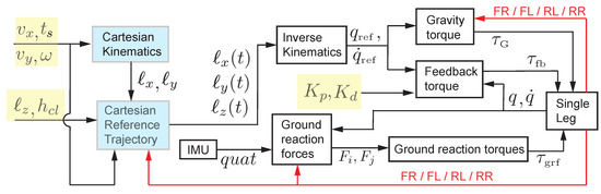
Figure 1.
Flowchart for the control of a single leg. The highlighted variables (in yellow) are the control variables: the torso speed in the fore–aft direction (), the torso speed in the lateral direction (), the angular velocity of the torso (), the leg height (), the ground clearance , and the step time . The highlighted blocks (in blue) are computed once per step (), while the others are set at 500 Hz. IMU stands for inertial measurement unit, and it provides the torso orientation as a quaternion (quat). Each of these blocks are elaborated in the low-level control section.
3.3. Cartesian Kinematics
The Cartesian kinematic block accepts inputs once per step, and it computes the fore–aft and lateral stepping lengths for the robot in the body frame. The body frame is defined as the frame that moves and rotates with the robot. The fore–aft direction is the x-direction, the lateral direction is the y-direction. The inputs to this block are the step time , the fore–aft speed in the body frame is , the lateral speed in the body frame is , and the rotation in the world z-frame is (pointing in the direction opposite of gravity). The step length for each of the diagonal pairs of legs in the fore–aft direction is and in the lateral direction is . However, for turning, the the rear legs have an additional lateral step length of .
3.4. Cartesian Reference Trajectory
The Cartesian reference trajectory generator block accepts inputs once per step, and it computes the fore–aft and lateral stepping trajectory as a function of time. The inputs to this block are the step length in the fore–aft direction , step length in the lateral direction , the leg height , and the ground clearance in the z-direction, . Using a fifth order polynomial, this block outputs the Cartesian trajectory for the foot as a function of time , , and .
3.5. Inverse Kinematics
The inverse kinematics block takes, as its input, the Cartesian position of the foot in the body frame , , and and outputs joint reference angles and angular velocities . These angles are the thigh roll , thigh pitch , and calf pitch as shown in Figure 2.
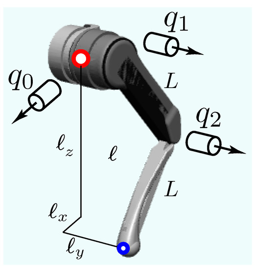
Figure 2.
Kinematics of a single leg.
If the Cartesian position of the foot is , then the forward kinematics model may be obtained as . For a given reference position , the joint angle is obtained by inverting as . The inverse, , is obtained analytically as follows. For a given end-effector position of the foot, , , and , the joint angles , , and may be found using the variables defined in Figure 2.
Note that , , and are intermediate variables for making the formulas short and succinct. The Jacobian of the foot with respect to the joint angles may be computed as follows, . Once the reference joint angle is computed, the reference joint velocity is given as follows .
3.6. Gravity Torque
The gravity torque compensation is used as a feedforward term for the swinging leg. The equation of motion of a single leg is given by where , , and are the mass matrix, Coriolis term, and gravity torque, respectively. The feedforward torque in the swing phase is given by ).
3.7. Ground Reaction Forces
The ground reaction forces block computes reference reaction forces on the two legs in contact with the ground assuming static equilibrium (i.e., no acceleration). Consider a point-mass model of the robot shown in Figure 3. This model assumes massless legs and that all the mass is concentrated at the torso. The inputs to this block are the torso orientation as a quaternion and all joint angles . The block outputs the reaction forces at the two feet and in the inertial frame (each force has x, y, and z components). Using the free body diagram, we have
where and are the position of the foot from the center of mass, and is the vector v written as a skew symmetric matrix. The total mass is , the corresponding mass matrix is , the inertia about the center of mass is , and the gravity vector is . Assuming that the torso has no linear acceleration, , or angular velocity, , the above equations may be simplified to
where and where is a identity matrix and is a vector of zeros, vector , and is the unknown force vector. Using the pseudo inverse, , we solve .
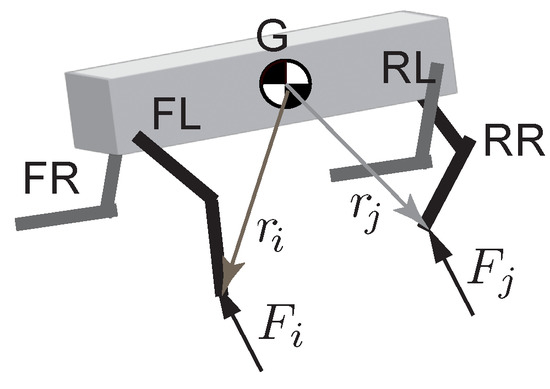
Figure 3.
Point-mass model to compute joint torques. The ground reaction forces are denoted by F and the location of the foot with respect to the center of mass of the torso is denoted by r.
3.8. Ground Reaction Torques
The ground reaction torque is used as a feedforward term to the leg on the ground. This block computes joint torques based on the ground reaction forces computed earlier. The ground reaction torque is given by where is the Jacobian.
3.9. Feedback Torque
The feedforward torques are supplemented with a feedback torque to achieve position control. This torque is given by where and are the user-chosen position and derivative gains. These gains were manually tuned in the following fashion. We set . Then, we ramped up until we obtained a sufficiently fast response. This led to an overshoot of the position. Then, the derivative gain was independently increased to avoid the overshoot and to ensure critical damping.
3.10. Single Leg Implementation
The finite state machine keeps track of the stance and swing legs. For the trot gait, the diagonal legs coordinate together and switch between being the stance and swing legs based on a fixed step time . This information is fed to the Cartesian trajectory generator to choose appropriate profiles for the legs and to the torque blocks to choose an appropriate torque. For the stance legs, the torque is given by , and for the swing legs, the torque is given by .
4. High-Level Control
4.1. Overview
The high-level control runs at the frequency of a step, . The velocity inputs are in the frame of the torso, the body frame. The inputs to the high-level control are the fore–aft speed in the body frame , the lateral speed in the body frame , the angular speed in the world frame , the leg height , and the ground clearance .
In open spaces, the robot is ideally operated in the velocity command mode where and or are set by the operator ( and are fixed). This allows the operator to intuitively control the robot. In constrained spaces, the robot needs to track suitable waypoints. These waypoints may be generated by the user or by a planner (e.g., A-star and RRT). Waypoint tracking takes place using feedback from the world coordinates of a suitable point on the robot () and the yaw angle of the torso (). Using the commands , , and , the controller can generate omnidirectional trotting.
4.2. High-Level Model
The robot has the ability to move in the fore–aft direction using , in the lateral direction using , and in the yaw direction using . This enables omnidirectional movement. The equations for the combined motion are the combination of the differential drive car motion () [33,34] and puck motion () [35] and are derived next.
The overall movement of the robot in the world frame may be described by the position of a point mid-way between the rear two legs in the world frame , ) and the orientation of the robot torso with respect to a suitably chosen reference x-axis in the world frame. Then,
4.3. High-Level Control
The feedback linearization control is given by where , , , and is a user-chosen gain matrix. Solving for the control
5. Results
5.1. Command following
Figure 4a shows the robot-tracking reference velocities and similar to a differential drive car [33,34], and Figure 4b shows the robot-tracking reference velocities and similar to a puck [35] as a function of the step number in simulation. The actual velocity is shown as solid red continuous line, and the reference velocity is shown as a dashed black line.
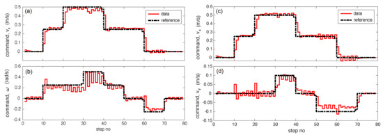
Figure 4.
Command following in simulation: (a,b) simultaneously command to follow and and (c,d) simultaneously commanded to follow and .
5.2. Waypoint Tracking
The leminscate (infinity symbol) is used as the reference trajectory.
where , , and a are suitable constants corresponding to the center and size of the lemniscate. The parameter , where t is the time, and is the end time. From these equations, one can compute and . The parameters were chosen as: m, , m, m, , and s. We consider two cases: (1) varying yaw: and (2) constant yaw . From these equations, the rate of change of the yaw can be computed as .
Figure 5 shows the results for varying yaw, where (a) is the simulation and (b) is the experiment, and the results for constant yaw, where (c) is the simulation and (d) is the experiment. These results were generated using a gain in simulation and in hardware, where is the identity matrix. We used an Optitrack motion-capture system consisting of 12 cameras to provide robot localization. The motion-capture system streams data at 300 Hz; however, we only need data at Hz.
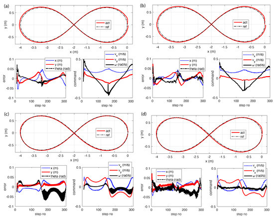
Figure 5.
Waypoint tracking of the robot: (a,b) show tracking for changing the yaw reference in simulations and experiments, respectively, and (c,d) show tracking for a constant yaw reference in simulations and experiments, respectively. Please see video [36].
From (a) and (b), it can be seen that the tracking errors in simulation and experiments in , , and are similar and within . From (c) and (d), it can be see that the tracking errors in simulation and experiments in and are similar and within , while those in are marginally higher in simulation compared with in experiments. There is ringing in the command in simulations, which shows up as ringing in the tracking of . The differences in the simulation/experiments are likely due to modeling errors, including friction. Please see the video (Figure 6) that compares the experiments with simulations [36].
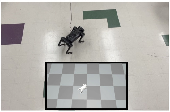
Figure 6.
A video that shows a comparison of the simulation (inset) with the hardware results (see video [36]).
6. Discussion
This paper presented a computationally simple trot controller that uses analytical solutions for inverse kinematics and feedforward torques. The resulting controller enabled omnidirectional trotting: forward/backward (), sideways (), and angular or turning motion (). Then, using the the three input commands (, , and ) and feedback linearization enabled waypoint tracking.
One of the advantages of legged locomotion over wheeled locomotion is the ability of legged robots to perform omnidirectional movement. Wheeled robots based on a steering drive and a differential wheel drive are subject to non-holonomic constraints, which prevent them from making sideways movements. In wheeled robots, this is overcome by using omni-directional wheels, which have rollers mounted on the wheels for sideways movement.
The morphology of the quadruped and the joint limits enable it to take larger steps and, consequently, to trot faster in the fore–aft direction compared with in the sideways direction. Thus, in order to move faster, it is more advantageous to turn in the direction of motion and use the fore–aft velocity command then to use the sideways mode of locomotion. However, in constrained spaces, it might be more advantageous to use the sideways mode of locomotion.
The low-level trot controller was based on analytical inverse kinematics, static-equilibrium-based feedforward compensation, and a simple proportional derivative position controller. This simple controller enabled fast computations on the hardware (worst case time of 2 ms but an average of ms on Raspberry PI). However, the use of static-equilibrium conditions to derive the controller also limited the speed of the robot to about 1 m/s in the fore–aft direction and m/s in the sideways direction with a 1 rad/s turning speed.
In order to increase the speed of the robot while using the same static-equilibrium conditions, one could change the step-level input from once per step to multiple times a step. This would enable increasing the feedback gain K and, hence, increase the speed of the robot.
7. Conclusions and Future Work
This paper demonstrated a simple trot controller with an analytical inverse and a combination of a static-equilibrium-based feedforward term and a position-velocity-based feedback term. The controller enabled versatile trot behaviors in the forward, backward, sideways, and turning directions, and all computations were conducted with an average time of ms. These trot behaviors—when suitably combined—can enable waypoint tracking. Future work will extend this to motion planning in constrained environments and to modifying the stepping control for disturbance rejection and high-speed navigation, including quick turning and quick acceleration.
Author Contributions
The authors made equal contributions to the paper. All authors have read and agreed to the published version of the manuscript.
Funding
The research was funded by the United States National Science Foundation through grants 1946282 and 2128568.
Data Availability Statement
Simulation code is available on https://github.com/pab47/quadruped/tree/main/a1_waypoint accessed on 17 December 2022.
Acknowledgments
The authors would like to thank Safwan Mondal for help with the motion-capture system and for videography.
Conflicts of Interest
The authors declare no conflict of interest. The funders had no role in the design of the study; in the collection, analyses, or interpretation of data; in the writing of the manuscript; or in the decision to publish the results.
References
- Raibert, M.; Chepponis, M.; Brown, H. Running on four legs as though they were one. IEEE J. Robot. Autom. 1986, 2, 70–82. [Google Scholar] [CrossRef]
- Marhefka, D.W.; Orin, D.E.; Schmiedeler, J.P.; Waldron, K.J. Intelligent control of quadruped gallops. IEEE/ASME Trans. Mechatron. 2003, 8, 446–456. [Google Scholar] [CrossRef]
- Pratt, J.; Dilworth, P.; Pratt, G. Virtual model control of a bipedal walking robot. In Proceedings of the International Conference on Robotics and Automation, Nagoya, Aichi, Japan, 21–27 May 1995; Volume 1, pp. 193–198. [Google Scholar]
- Chen, G.; Guo, S.; Hou, B.; Wang, J. Virtual model control for quadruped robots. IEEE Access 2020, 8, 140736–140751. [Google Scholar] [CrossRef]
- Arena, P.; Patanè, L.; Taffara, S. Energy efficiency of a quadruped robot with neuro-inspired control in complex environments. Energies 2021, 14, 433. [Google Scholar] [CrossRef]
- Liu, C.; Chen, Q.; Xu, T. Locomotion control of quadruped robots based on central pattern generators. In Proceedings of the 2011 ninth World Congress on Intelligent Control and Automation, Taipei, Taiwan, 21–25 June 2011; pp. 1167–1172. [Google Scholar]
- Park, H.W.; Park, S.; Kim, S. Variable-speed quadrupedal bounding using impulse planning: Untethered high-speed 3d running of mit cheetah 2. In Proceedings of the 2015 IEEE International Conference on Robotics and Automation (ICRA), Seattle, WA, USA, 26–30 May 2015; pp. 5163–5170. [Google Scholar]
- Ding, Y.; Pandala, A.; Park, H.W. Real-time model predictive control for versatile dynamic motions in quadrupedal robots. In Proceedings of the 2019 International Conference on Robotics and Automation (ICRA), Montreal, QC, Canada, 20–24 May 2019; pp. 8484–8490. [Google Scholar]
- Di Carlo, J.; Wensing, P.M.; Katz, B.; Bledt, G.; Kim, S. Dynamic locomotion in the mit cheetah 3 through convex model-predictive control. In Proceedings of the 2018 IEEE/RSJ International Conference on Intelligent Robots and Systems (IROS), Madrid, Spain, 1–5 October 2018; pp. 1–9. [Google Scholar]
- Zheng, A.; Narayanan, S.S.; Vaidya, U.G. Optimal Control for Quadruped Locomotion using LTV MPC. arXiv 2022, arXiv:2212.05154. [Google Scholar]
- Chi, W.; Jiang, X.; Zheng, Y. A linearization of centroidal dynamics for the model-predictive control of quadruped robots. In Proceedings of the 2022 International Conference on Robotics and Automation (ICRA), Philadelphia, PA, USA, 23–27 May 2022; pp. 4656–4663. [Google Scholar]
- Kang, D.; De Vincenti, F.; Coros, S. Nonlinear Model Predictive Control for Quadrupedal Locomotion Using Second-Order Sensitivity Analysis. arXiv 2022, arXiv:2207.10465. [Google Scholar]
- Hamed, K.A.; Kim, J.; Pandala, A. Quadrupedal locomotion via event-based predictive control and QP-based virtual constraints. IEEE Robot. Autom. Lett. 2020, 5, 4463–4470. [Google Scholar] [CrossRef]
- Chen, S.; Zhang, B.; Mueller, M.W.; Rai, A.; Sreenath, K. Learning Torque Control for Quadrupedal Locomotion. arXiv 2022, arXiv:2203.05194. [Google Scholar]
- Lee, J.; Hwangbo, J.; Wellhausen, L.; Koltun, V.; Hutter, M. Learning quadrupedal locomotion over challenging terrain. Sci. Robot. 2020, 5, eabc5986. [Google Scholar] [CrossRef] [PubMed]
- Peng, X.B.; Coumans, E.; Zhang, T.; Lee, T.W.; Tan, J.; Levine, S. Learning agile robotic locomotion skills by imitating animals. arXiv 2020, arXiv:2004.00784. [Google Scholar]
- Bellegarda, G.; Nguyen, Q. Robust high-speed running for quadruped robots via deep reinforcement learning. arXiv 2021, arXiv:2103.06484. [Google Scholar]
- Tan, J.; Zhang, T.; Coumans, E.; Iscen, A.; Bai, Y.; Hafner, D.; Bohez, S.; Vanhoucke, V. Sim-to-real: Learning agile locomotion for quadruped robots. arXiv 2018, arXiv:1804.10332. [Google Scholar]
- Kumar, A.; Fu, Z.; Pathak, D.; Malik, J. Rma: Rapid motor adaptation for legged robots. arXiv 2021, arXiv:2107.04034. [Google Scholar]
- Li, H.; Yu, W.; Zhang, T.; Wensing, P.M. Zero-shot retargeting of learned quadruped locomotion policies using hybrid kinodynamic model predictive control. In Proceedings of the 2022 IEEE/RSJ International Conference on Intelligent Robots and Systems (IROS), Kyoto, Japan, 23–27 October 2022; pp. 11971–11977. [Google Scholar]
- Fawcett, R.T.; Afsari, K.; Ames, A.D.; Hamed, K.A. Toward a data-driven template model for quadrupedal locomotion. IEEE Robot. Autom. Lett. 2022, 7, 7636–7643. [Google Scholar] [CrossRef]
- Dudzik, T.; Chignoli, M.; Bledt, G.; Lim, B.; Miller, A.; Kim, D.; Kim, S. Robust autonomous navigation of a small-scale quadruped robot in real-world environments. In Proceedings of the 2020 IEEE/RSJ International Conference on Intelligent Robots and Systems (IROS), Las Vegas, NV, USA, 24 October 2020–24 January 2021; pp. 3664–3671. [Google Scholar]
- Chilian, A.; Hirschmüller, H. Stereo camera based navigation of mobile robots on rough terrain. In Proceedings of the 2009 IEEE/RSJ International Conference on Intelligent Robots and Systems, St. Louis, MO, USA, 10–15 October 2009; pp. 4571–4576. [Google Scholar]
- Karydis, K.; Poulakakis, I.; Tanner, H.G. A navigation and control strategy for miniature legged robots. IEEE Trans. Robot. 2016, 33, 214–219. [Google Scholar] [CrossRef]
- Kim, Y.; Kim, C.; Hwangbo, J. Learning Forward Dynamics Model and Informed Trajectory Sampler for Safe Quadruped Navigation. arXiv 2022, arXiv:2204.08647. [Google Scholar]
- Guizzo, E.; Ackerman, E. $74,500 will fetch you a spot: For the price of a luxury car, you can now buy a very smart, very capable, very yellow robot dog. IEEE Spectr. 2020, 57, 11. [Google Scholar] [CrossRef]
- Hutter, M.; Gehring, C.; Jud, D.; Lauber, A.; Bellicoso, C.D.; Tsounis, V.; Hwangbo, J.; Bodie, K.; Fankhauser, P.; Bloesch, M.; et al. Anymal-a highly mobile and dynamic quadrupedal robot. In Proceedings of the 2016 IEEE/RSJ International Conference on Intelligent Robots and Systems (IROS), Daejeon, Republic of Korea, 9–14 October 2016; pp. 38–44. [Google Scholar]
- Unitree-Robotics. A1 More Dexterity, More Possibilities. 2022. Available online: https://www.unitree.com/products/a1/ (accessed on 17 December 2022).
- Katz, B.; Di Carlo, J.; Kim, S. Mini cheetah: A platform for pushing the limits of dynamic quadruped control. In Proceedings of the 2019 International Conference on Robotics and Automation (ICRA), Montreal, QC, Canada, 20–24 May 2019; pp. 6295–6301. [Google Scholar]
- Kau, N.; Bowers, S. Stanford Pupper: A Low-Cost Agile Quadruped Robot for Benchmarking and Education. arXiv 2021, arXiv:2110.00736. [Google Scholar]
- Kau, N.; Schultz, A.; Ferrante, N.; Slade, P. Stanford doggo: An open-source, quasi-direct-drive quadruped. In Proceedings of the 2019 International Conference on Robotics and Automation (ICRA), Montreal, QC, Canada, 20–24 May 2019; pp. 6309–6315. [Google Scholar]
- Grimminger, F.; Meduri, A.; Khadiv, M.; Viereck, J.; Wüthrich, M.; Naveau, M.; Berenz, V.; Heim, S.; Widmaier, F.; Flayols, T.; et al. An open torque-controlled modular robot architecture for legged locomotion research. IEEE Robot. Autom. Lett. 2020, 5, 3650–3657. [Google Scholar] [CrossRef]
- LaValle, S.M. Planning Algorithms; Cambridge University Press: Cambridge, UK, 2006. [Google Scholar]
- Sanchez, S.; Bhounsule, P.A. Design, Modeling, and Control of a Differential Drive Rimless Wheel That Can Move Straight and Turn. Automation 2021, 2, 6. [Google Scholar] [CrossRef]
- Hackett, J.; Gao, W.; Daley, M.; Clark, J.; Hubicki, C. Risk-constrained motion planning for robot locomotion: Formulation and running robot demonstration. In Proceedings of the 2020 IEEE/RSJ International Conference on Intelligent Robots and Systems (IROS), Las Vegas, NV, USA, 24 October–24 January 2021; pp. 3633–3640. [Google Scholar]
- Bhounsule, P.A. A simple Controller for Omnidirectional Trotting of Quadrupeds: Command Following and Tracking. 2022. Available online: https://youtu.be/o8qkcMmQTQI (accessed on 17 December 2022).


Disclaimer/Publisher’s Note: The statements, opinions and data contained in all publications are solely those of the individual author(s) and contributor(s) and not of MDPI and/or the editor(s). MDPI and/or the editor(s) disclaim responsibility for any injury to people or property resulting from any ideas, methods, instructions or products referred to in the content. |
© 2023 by the authors. Licensee MDPI, Basel, Switzerland. This article is an open access article distributed under the terms and conditions of the Creative Commons Attribution (CC BY) license (https://creativecommons.org/licenses/by/4.0/).