Abstract
Sheet metal parts can often replace milled components, strongly improving the buy-to-fly ratio in the aeronautical sector. However, the sheet metal forming of complex parts traditionally requires expensive tooling, which is usually prohibitive for low manufacturing rates. To achieve precise parts, non-productive and cost-intensive geometry straightening processes are additionally often required after forming. Rollforming is a possible technology for producing profiles at large rates. For low manufacturing rates, robotic rollforming can be an interesting option, significantly reducing investment at the cost of higher manufacturing times while keeping a high process flexibility. Forming is performed incrementally by a single roller set moved by the robot along predefined bending curves. The present work’s contribution to the overall solution is the development of an intelligent algorithm to calculate geometry after a robotic rollforming process based on process reaction forces. This information is required for in-process geometric distortion correction. Reaction forces and torques are acquired during the process, and geometry is calculated based on artificial intelligence (AI) applied to that information. The present paper describes the AI development for this virtual geometry sensing system.
1. Introduction
Depending on the detailed part design, replacing milled parts with sheet metal parts can strongly improve complex structures’ ecoefficiency due to much more efficient material usage. Traditionally, efficient sheet metal forming requires rather expensive machines and tooling. This makes the process most suitable for high-rate production, e.g., in the automotive industry. Milled parts, on the contrary, can be produced with a similar efficiency at very low manufacturing rates. One way to implement sheet metal forming for low production rates is to develop suitable incremental forming processes based on adaptable tooling solutions [1]. Instead of designing and implementing complex and cost-intensive forming tools, incremental forming processes with rather simple tools and tool paths are adapted to changing tasks. A technology that illustrates this point well is rollforming. In accordance with the DIN8580 classification [2], it is characterized as bending with rotating tools that are subsequently aligned on multiple forming stands. Rollforming has undergone a tremendous flexibilization process in the past years. While conventional rollforming is suitable for producing large volumes of profiles with constant cross sections cost-efficiently, it requires large rollforming machines and individual roll sets with a defined number n of forming passes for each profile [3]. Solutions for flexible rollforming already exist in research and industrial applications, e.g., from companies such as dataM [4,5,6] and Ortic [7]. In each case, the main objective is to produce complex rollformed sheet metal parts with variable cross sections in width and even in depth. Production rates using such a setup with multiple roll sets can be comparable to simple rollformed parts in a continuous process. Due to time-consuming adaptions, e.g., changeover of rolls and necessary initial measurements when forming new parts, this might, however, not be suitable for the prototyping of components [8] or otherwise very low production rates. Additionally, it comes at a high machinery cost due to the required number of adaptable axes for all required rollforming stands. The setup and commissioning complexity is very high, which leads to a significant amount of material required to achieve the first part within the required tolerances. The novel robotic rollforming (RoRoFo), as first described by Richter et al. [9] is a technology approach that minimizes the deployed machinery and tooling. The rolls are attached to a robotic end-effector. They are moved along the bending edge several times by the industrial robot, comparable to the number n of forming passes needed for conventional rollforming. A higher labor time per part is frequently acceptable for a low-rate but highly flexible production. The much more adaptable RoRoFo process aims at a first-time-right strategy for very low manufacturing rates.
Using sheet metal forming instead of milling thin-walled parts from a solid plate not only saves material, but has the potential to even enhance material properties. Depending on the material used, deforming grains usually leads to better mechanical performance than cutting grains [10] coming along with strain hardening during forming. Solid metal plates usually contain non-uniform grain structures across the thickness, with partially lower properties expected at the surface. Milling very thin structures out of thick material plates may furthermore lead to reduced fatigue properties since a significant part of the final component is machined from volumes close to the original plate surface [11]. In terms of design, however, milling provides more freedom of choice regarding the design. This includes features such as integrated ribs, which improve mechanical performance. When changing the manufacturing process from milling to forming for a specific component, a thorough redesign is thus required. The design has to be optimized taking into account formability, yet has to fulfill all requirements met by the original part as well. Therefore, changing the manufacturing process is a complex task due to the high impact on part design.
Results of rollforming are strongly influenced not only by fairly predictable springback, but, among others, also by residual stresses induced by previous processes, which can only be predicted to a limited extent, especially in incremental forming processes. Prediction of springback by artificial intelligence (AI) has been studied in other works, trained with simulation data. In the present work however, the focus is on the determination of geometry errors due to fewer predictable factors for straightening purposes using actual process data. It is well understood that flexible roll forming processes may lead to geometrical imperfections, e.g., wrinkles and end flare [12,13,14], which is especially true when processing high-strength steels. Additionally, sheet metal parts may react differently to the same process due to small differences between material batches [15,16] Geometry wise, the thickness of sheets may slightly differ within the allowed tolerances. More importantly, however, and very difficult to detect before processing a part, the residual stress profile in rolled sheet metal parts can differ from part to part [17]. Thus, it is important to develop the RoRoFo process, including the capability of reacting to the material behavior of the actual part being processed close to real time. Traditional rollforming solutions, which mainly rely on a rigid and well-defined roller setup, often require a geometrical calibration step at the end of the rollforming line [18,19,20]. The high degree of freedom of a robotic process during forming makes it even more important to develop an in-process compensation strategy. In the present case, the goal is to integrate a roller-based straightening process directly in the forming process, which allows optimizing the obtained geometry in the direction of the final geometry defined in the initial drawings. Straightening shall be based on an AI solution due to its complex nature, and this more intelligent process is denoted as iRoRoFo from now on [21,22,23].
In order to achieve the final goal of an industrially robust first-time-right process, a virtual geometry sensing approach is required, which can directly use the force feedback available to the robot in order to acquire the obtained part geometry at any production increment without interrupting the process and without relying on challenging optical geometry measurement solutions. The relationship between measured forces and geometry cannot be easily calculated analytically [16]. AI algorithms might serve to calculate the geometry. The present work focuses on this sensing solution. It is developed on a series of thin steel metal sheets with a well-defined sinusoidal target geometry.
2. Materials and Methods
In the iRoRoFo process, a sheet is formed by a robotic end-effector consisting of two rollers. During the process, forces at the robot flange are recorded, and after forming the required geometry correction is calculated and applied in the final forming increment. The geometry is measured by an external system for developing the force based geometry measurement solution. Figure 1 describes the corresponding process flow starting at a flat sheet, which is incrementally formed and straightened. The upper three sketches represent the process steps discussed herein, whereas the lower three sketches represent the rest of the process chain still being developed.
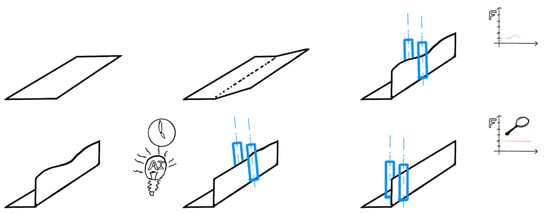
Figure 1.
iRoRoFo-process sequence.
2.1. Robotic Cell Setup
The KUKA KR150 R2700 extra [24] robot shown in Figure 2, including the software technology package KUKA.RobotSensorInterface RSI [25], was used for the trials. The package is designed for cyclical communication with the robot and enables data acquisition at the robot interpolation rate of 4 ms. In particular, using RSI instead of an independent data acquisition system for process forces for the presented application has the advantage that positions of axes and of the tool center point are registered together with the sensor data. A Schunk FT160 SI-2500-400 load cell is installed at the robot flange and connected to the sensor interface. This setup allows recording reaction forces on the end-effector in 6 axes during the forming process. Specimens are clamped between rigid steel plates in a position that allows forming and geometrical measurements.
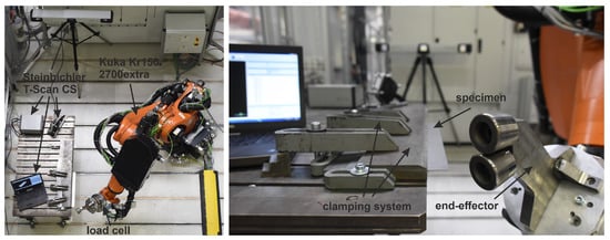
Figure 2.
Cell setup used for the experiments.
The used prototypical end-effector consists of a solid plate that allows for the fixation to the robot flange. Two conical rolls with a maximum diameter D of 60 mm are fixed with a shoulder screw with a collar (ISO 7379) each. The gap between the rolls is fixed at 1.6 mm, i.e., roll diameters have to be adapted when changing the sheet metal thickness. The two rolls are conical with an angle of = each, thus allowing for a maximum cumulative bending of when starting with flat sheets. The geometrical conditions of the rolls as implemented in the experimental setup are shown in Figure 3. The upper roll of the end-effector touched the specimen mainly in the bending corner, whereas the lower roll supported the full sheet-flange height to be bent upwards. The radius of the rolls defining the bending edge was r = 3 mm.
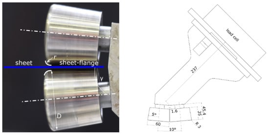
Figure 3.
Scheme of robotic end-effector.
In the foreground of the right picture of Figure 2, the clamping solution for the sheet metal to be formed during the trials is shown. The sheet was rigidly clamped between two steel plates secured by clamping claws with a cantilever length of 42 mm. At a flange angle of (corresponding to the sixth bending increment), the upper plate was moved back by the roller diameter of 60 mm to create the required space for further bending and preventing collisions between the upper roll and the blank holder.
2.2. Specimen
Experiments were performed using blanks of a high-strength steel. Based on widely available pearlite-reduced, microalloyed hot-rolled steel strips, the ZE760 material combines reliable, and high-precision cold-rolling and heat treatment strategies [26,27]. Table 1 shows the chemical composition of the chosen sheet material. The used sheets had a nominal thickness of 1.54 mm with a tolerance of +0.06 mm.

Table 1.
Chemical composition in weight percentage of the sheet material.
Rectangular blanks with a length of 524 mm and a width of 200 mm were prepared using a cutting press with subsequent deburring of all edges.
2.3. Process
The iRoRoFo process was developed for arbitrary sheet geometries. For development purposes, however, it was initially decided to develop the solution with a simplified and well-defined geometry. A sketch of the target geometry to be incrementally formed is shown in Figure 4. The flange angle used for analysis is denoted as . The constant angle to be achieved is denoted as , and the error applied on purpose is along the bending edge with the shape of a sinusoidal wave as (wave amplitude is ). Additionally, at any location along the bending edge, an unintentional angular error may occur, e.g., due to residual stresses present in the sheet before forming. The length of the bent edge is designated as ‘w’, while the wavelength of the applied wave is ‘a’. Bending occurs around the upper roller radius, therefore locally lengthening the sheet across its cross section. The axis of the rolls is oriented perpendicularly to the bending edge.
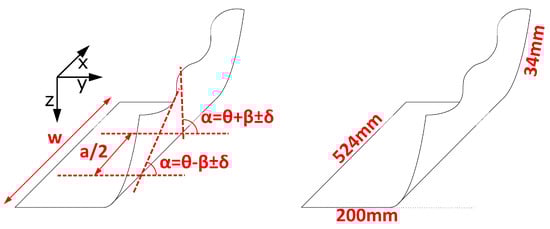
Figure 4.
Scheme of the defined specimen.
The forming process starts with a flat sheet featuring a length of 524 mm and consists of three stages, which are illustrated in Figure 5. In Forming stage 1, a constant bending angle of minus the elastic springback is incrementally created starting with a flat sheet. The angular increment corresponding to for each forming step is gradually introduced along the full bending edge length (1). The increment angle is applied to the entire sheet length on the way back (2). This procedure was repeated up to an angle of (3). In order to avoid collision with both the blank holder and the clamping system, the clamping was relocated after forming up to as described before. Elastic springback after forming up to (4) was allowed to occur as the rollers were moved entirely out of the sheet. The geometry of the sheet obtained after the final iteration of forming stage 1 was measured, and the average obtained angle was determined to be approximately , i.e., the springback amounted to . The tool angle was adjusted from to before moving back into the sheet in order to avoid a collision. In Forming stage 2, a sinusoidally wave was applied to the bent edge (5). The corresponding tool path was defined as a sinusoidal curve consisting of 5 waves with a wavelength of 104.8 mm and an amplitude of oscillating around a mean value of (i.e., the resulting angle after the first forming stage including springback). In Forming stage 3, the tool followed a straight path back to the sheet start at a constant bending angle of . The reaction forces and torques corresponding to the varying elastic response of the formed sheet during backward movement were recorded (6). These data were used later for virtual geometry measurement. Reference geometry measurements were performed, and afterward, the sheet was unclamped, achieving its final geometry after release.
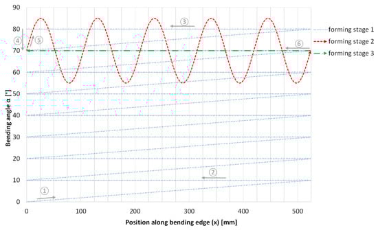
Figure 5.
Scheme of forming path for all increments.
In order to provide sufficient data for training and validating the AI algorithms, twelve sampled were prepared following the described process.
2.4. Reference Geometry Measurement System
The device Steinbichler T-Scan CS was used for reference geometry measurements (Figure 2 background). In order to evaluate the results of the forming process and to generate reference values for the virtual sensing solution, the geometry was recorded by a hand-held laser line scanner after forming. For this purpose, the sheet metal part was scanned several times from different angles, obtaining a point cloud. This optical measurement method can be influenced by many factors, including the material’s reflection and the laser scanner’s angle in relation to the measured surface. High-quality measurements were possible on the used samples. However, a three-dimensional point cloud contains too much information for automatic interpretation considering the low number of trials. Therefore, the flange angle along the bending edge, extracted from the point cloud following the approach described in Section 2.5, was chosen for describing the most relevant features of the sheet geometry.
2.5. Angle Measurement Data
The measured geometry was evaluated after forming. In order to calculate flange angle , the evaluation of the recorded point clouds was performed according to the following steps:
Cleaning: The recorded point cloud contained geometrical information regarding the surrounding of the part to be measured as well as measurement artifacts, all of which were removed in post-processing.
Geometrical alignment: The point clouds were aligned along their main axes for comparability and compatibility with the developed analysis algorithm.
Export: The measured and pre-processed point cloud was exported in ASCII format for further post-processing.
Data extraction: The flange angle along the bending edge (direction x shown in Figure 4) was determined automatically using a specifically developed algorithm. A line vertical to the edge of the sheet metal was first defined for every 10 mm of the bending edge. The points from the cloud closest to this line were chosen; thus, a section was defined for each 10 mm. This section was then projected on a plane. It can be divided into the clamped sheet region and the bent sheet. Lines were automatically fitted to these areas based on linear regression, and the angle between the regression lines was determined; see Figure 6. The automatically determined results were randomly checked along the entire bending edge by manual measurements.
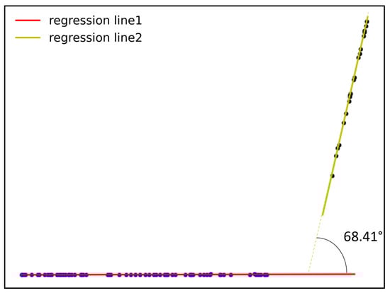
Figure 6.
Extracted geometry points for one cutting plane with regression lines at x = 434 mm.
2.6. Force Measurement Data
Reaction forces and torques were measured in three axes using the sensor attached to the robot flange during the forming process. Since the measured forces are influenced by various parameters that are not related to forming (such as the tool’s weight force), a concept was developed to eliminate those and focus on the reaction forces caused by the forming process itself. This concept consists of subtracting the forces acquired during an empty run, i.e., performing the same robot path without a sheet metal to be formed, from the measured forces during forming. In the last step, the preprocessed measurement data were filtered to remove noise. The process flow is shown in Figure 7.
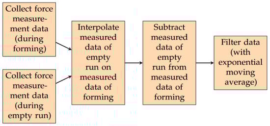
Figure 7.
Force measurement data preprocessing scheme.
Each forming step consists of forward and backward movements. If the same path is followed in both directions, it may be expected that plastic and elastic deformation occur during forward movement and elastic deformation during backward movement. As described before, in forming stage 2, a sinusoidal path is used for the forward movement, and a straight path is used for the backward movement in forming stage 3. During backward movement, forces may occur in both positive and negative directions, originating from the mainly elastic reaction due to the sinusoidal path. The following discussion is limited to the straight path in the backward direction after the final sinusoidal path.
3. Results
As previously explained, the present study aims to use the force measurement device at the robotic end-effector as a virtual geometry sensor for the bent sheet. For this purpose, data preprocessing was performed for the force as well as for the reference geometry measurement data. Repeatability was examined, and the correlation between the parameters was investigated. Different algorithms, including support vector regression, random forest, and neuronal networks were trained on the prepared data, and the results were compared. In general, hyperparameters have a significant influence on the results. This becomes especially complicated when several hyperparameters have to be selected for training neural networks. Therefore Optuna [28] was used for hyperparameter tuning. The corresponding results are presented in this section.
3.1. Repeatability
Before evaluating and analyzing the data in detail, the repeatability of the performed experiments was checked. Figure 8 shows the flange angle along the bending edge for 12 samples, as this is the most relevant geometrical feature extracted from the acquired data. It proves good repeatability of the specimen shape if rarely occurring outliers that are linked to measurement artifacts are disregarded. Such artifacts may, for instance, originate from the unwanted reflection of the laser used for geometry acquisition. Instead of removing all outliers manually before proceeding, the present work aims at developing a robust method capable of handling such artifacts common also in industrial measurements.
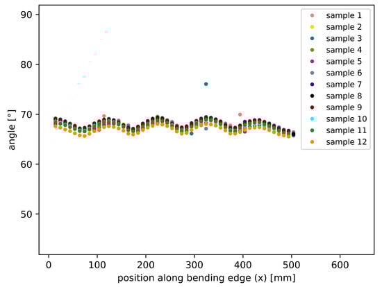
Figure 8.
Measured angles along the bending edge.
However, the results partially present a slight offset of the complete curve, most likely resulting from slight differences in the specimen.
Figure 9 exemplarily shows the force measurement data in the X direction along the bending edge for the same twelve samples.
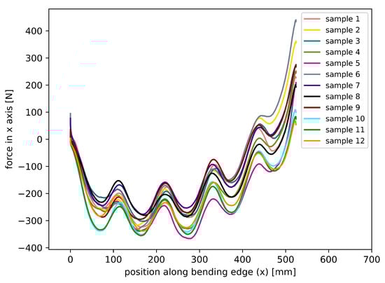
Figure 9.
Repeatability of measured forces in X direction along the bending edge.
A similar general pattern can be recognized in the measured forces, although oscillating around an unknown base function and with a variable offset along the bending edge. The constant distance between the used rollers and the allowed sheet thickness tolerances might explain the differences. The combination of both cannot guarantee constant contact between rollers and the sheet.
The force measurement system was reset to zero post-processing at the last contact point between the rollers and the sheet near x = 0 mm. In that location, the bending angle is , and elastic springback is, therefore, minimized. This is also the best moment to guarantee similar boundary conditions between all samples, even considering manufacturing and setup tolerances.
The diagram shown in Figure 9 is selected exemplarily only. Similar behavior can be seen when examining the force in the other axes and torques around all axes (see Figure 10). The oscillation emerges for all observed force directions but around different base functions and with different amplitudes. This means that not all force directions are affected similarly by the measured geometry, which is discussed in Section 3.2. Measured force evolution curves along the bending edge may be sufficiently repeatable.
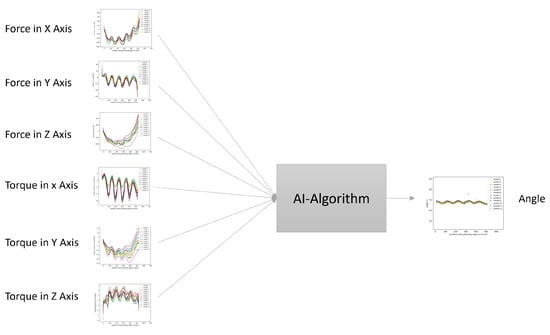
Figure 10.
Structure of input and output data.
3.2. Model Selection
After data preprocessing, the structure of data input and output can be defined as shown in Figure 10. The goal is to find a suitable model to predict the angle along the bending edge of the sheet (right side) using the available input data (left side).
We assume that there is a correlation between the externally measured geometry and internally measured force. However, there is no direct and easily recognizable rule for this correlation. For this reason, AI algorithms were used for data analysis. When selecting inputs and outputs for AI algorithms, it is desired that there is a relationship between inputs and outputs. However, the same is not valid without restriction for different input data. For checking possible relationships between different input data, the correlation between them was analyzed by calculating the Pearson correlation coefficient, which is a linear correlation coefficient for measuring the association between two variables [29]. The input data consist of forces and torques in the x, y and z directions along the bending edge. The highest correlation was found between the force on the y-axis and torque on the x-axis, with a value of 0.93. Force in the z-axis also correlates highly with force in the x-axis and torque in the y-axis. The mentioned correlations have values equal to 0.89 and 0.82. The Pearson factor was also calculated between input and output data, but no significant values could be detected. This was expected since there is no visible linear relationship between input and output. Since there is no clear understanding of whether and which parameter should be eliminated from the input data set to achieve even better results with machine learning (ML) algorithms, the complete data were used in the present work. Further research could be performed in this context, exemplarily by bivariant feature analysis and also with the help of principal component analysis.
By comparing the accuracy of different machine learning methods, insights into the appropriate algorithm choice for this problem can be provided. In order to compare the algorithms with the same training and test data, the measured data were divided into training data for the ML model containing the measured data from eleven experiments and training data only consisting of the measured data from one sample.
The first algorithm tested was a random forest model, which includes many decision trees trained on different subsets of the training data. The final prediction is made by aggregating the predictions of the individual trees. Figure 11 shows the results obtained with this algorithm. In the left diagram, the training data are marked with orange dots and the prediction with green stars. It can be seen that in the training phase itself, the outliers are learned, and thus the prediction becomes less accurate. On the right diagram, the results of the test are shown, where the measured data are marked in blue and the predicted data in red. It can be seen that the pattern is roughly predicted, but the peak values are not close enough to the measured test data. To evaluate the performance of models, different metrics can be applied. This work compares the models with MSE (mean squared error) and MAE (mean absolute error), which both take non-negative values, and the goal of a model is to minimize them. Significant errors are usually overestimated with MSE. Therefore, MAE was additionally used for analysis as a supplement. For the discussed model, values 0.85 and 0.93 were obtained for the MAE and MSE of the test data. Therefore, an average prediction error of was found, and there was no significant outlier that strongly increased the MSE. This can also be seen in the diagrams in Figure 11.
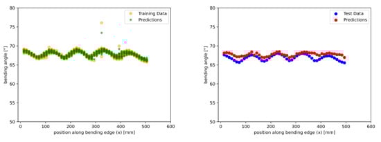
Figure 11.
Geometry prediction results with random forest regression.
Support vector regression was the next tested ML algorithm, which has several advantages, including the ability to handle high-dimensional data and its robustness against noise and outliers. It can be seen in the prediction results shown in Figure 12 that the outliers are not learned. Compared to the previous algorithm, prediction is improved, and lower MSE and MAE for test data are obtained, with values of 0.66 and 0.73.
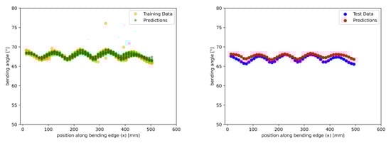
Figure 12.
Geometry prediction results with support vector regression.
The relationship between the achieved geometry after forming and measured reaction forces were also studied previously [30]. There the geometry prediction was investigated for a constant angle along the bending edge and, therefore, different from the present analysis. Contrary to the present work, where the forward and backward movements were different during forming, in previous work [30], the same path was followed in both directions. In that case, the best result was achieved by using neural networks. The same approach was tested in the presented work but strongly improving the tuning of parameters used to control the learning process in relation to that work. Hyperparameter tuning was implemented using Optuna, testing different hyperparameters in a user-defined range and test number. Since Optuna uses training and validation sets for each test procedure, a separate test dataset was defined. Thus, the grouping of datasets was changed compared to the previously presented algorithms. Similar to the other algorithms, a single sample was separated for testing the model at the end. In total, 75% of the remaining datasets were used for training and the rest for validation during hyperparameter tuning. There are different methods for hyperparameter tuning, each with its own advantages and disadvantages. In this work, the TPE (tree-structured Parzen estimator) [31] sampler was chosen, which uses previous experience of evaluated hyperparameters to create a probabilistic model and to suggest a next set of hyperparameters. Hyperparameter tuning can strongly influence the results of neural networks. However, this can also lead to overfitting so that the prediction for training data is perfect, but the model cannot deliver good results for new data. Therefore, hyperparameter tuning provides values for parameters that allow good predictions, simultaneously preventing overfitting. Unpromising sample data were also removed during the hyperparameter tuning. Table 2 shows the defined search space. The topology of the neural network is defined by the number of layers and the number of neurons per layer. With activation function the output of each layer is calculated, and dropout is a technique to avoid overfitting. Learning rate defines the step size to update parameters, and epochs define the number of cycles to train the model. The batch size defines the number of training samples that pass through to the network at a time.
Table 2.
Definition of search space for hyperparameters.
Figure 13 shows the results of hyperparameter tuning. On the left diagram, the progress can be seen, where the blue dots represent MSE in each sample, and the red line illustrates the best-achieved value. As shown in the diagram, the red line decreases until the marked location, and then it is almost constant. This is also confirmed in the summary report, which indicated that the best test was obtained in test 537, with an MSE value of 0.097. This MSE was determined with the test data containing 25% of measurement data from 11 samples. The diagram on the right shows the relative importance of different hyperparameters for MSE. The number of layers is the parameter with highest influence on MSE. Epochs as well as number of neurons in the first and last hidden layers follow with a significant distance, and thus together are the most important hyperparameters.
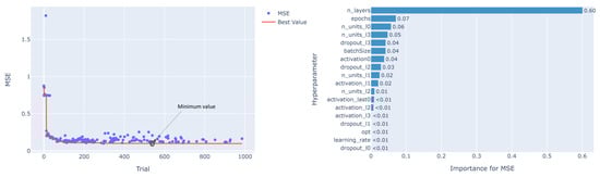
Figure 13.
Results of hyperparameter tuning.
The following analyses investigated the influence of batch size, epochs, number of layers, and learning rate on MSE. The achieved MSE as a function of hyperparameter values in each sample is first shown in Figure 14. On the x-axis, the values of each hyperparameter and on the y-axis, the achieved MSE are shown, and the different blue tones of the points are supposed to indicate different samples. Since in this diagram, for each sample, only the single hyperparameter is shown and the values of other hyperparameters in the sample are not visible, in Figure 15, the selected combination of them in each sample is shown in a single view. So, in the first diagram, the more exact values and the development in each experiment can be analyzed. In the second diagram, the influence in combination with other hyperparameters can be shown together.
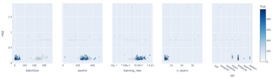
Figure 14.
Slice plot of hyperparameters.
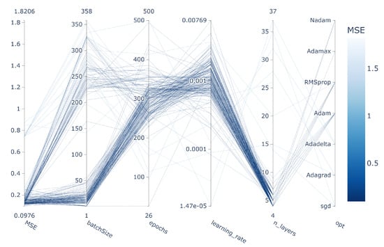
Figure 15.
Parallel coordinate plot of hyperparameters.
It can be seen that small values of MSE can be achieved with smaller batch sizes (1–70) as well as larger ones (200–300). However, best values are achieved with a batch size smaller than 70, which also causes longer training times. Epoch numbers between 200 and 400 and a learning rate between 0.0005 and 0.007 also have an impact on better results. A small number of layers between 4 and 10 has shown a positive influence. Most of the good results were achieved using RMSprop as an optimizer.
After 1000 runs, the best-proposed model is a neural network with 4 hidden layers trained in 262 epochs with a batch size equal to 9. To compare the results with the other models, the flange angle along the bending edge was plotted for measured and predicted data; see Figure 16. When looking at the training data (left plot), it can be seen that outliers are not learned, but the predictions for x-values in the range of 400 mm and higher contain higher errors. On the right plot, the test data show that the pattern was predicted much better compared to the other proposed models. Especially at the beginning and end of the sheet, the curve direction could be predicted better, and in the middle of the sheet, there is a lower error. This is confirmed by a MSE value of 0.22 and a mean absolute error (MAE) of .
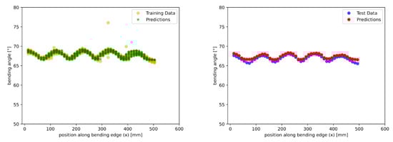
Figure 16.
Geometry prediction results with the neural network.
Figure 17 shows a detailed view of the right graph in Figure 16. It can be seen that the prediction error is generally below and that there is a slight positive offset in the predicted data. The offset in the prediction may be due to slight errors in the measurement of the springback during forming trials and the fact that the load cell was reset with the end-effector on the sheet adjusted to , taking into account this springback. The reference geometry was measured without force applied to the sheet flange. In the middle of the sheet, around x = 300 mm, the highest similarity between the predicted and measured data was found. The error at the beginning and end of the sheet was higher, similar to the results obtained with the other algorithms. This could be because the forming behavior in those areas is mechanically different from the central part since there is no material continuity before and after the sheet. Neural networks were, however, able to predict even these critical areas with reasonable precision.
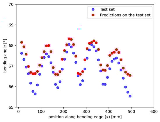
Figure 17.
Zoom into the geometry prediction results shown in Figure 16.
Table 3 summarizes the achieved metrics for the tested algorithms.
Table 3.
Comparison of metrics for different algorithms.
4. Discussion and Outlook
Industrial application of the RoRoFo process necessarily leads to a trade discussion between the process lead time, initial investment and process adaptability. The iRoRoFo process further allows optimizing or even eliminating the non-value-adding straightening process, thus reducing the production time. The processing time is expected to be between the machining of complex parts and traditional sheet metal forming processes. The combination of high geometrical adaptability and low initial investment, however, makes it suitable for an industrial application in areas with complex roll-formed parts and low manufacturing rates.
Using a force-based virtual sensor for geometry acquisition allows achieving robust in-line geometry measurements, even in an industrial environment. Since in the present setup, the force is measured directly at the robot flange and the applied forces are well below the robot capabilities, the measurement results are not influenced by the robot’s intrinsic reduced stiffness. A combination of methodically optimized robotic stiffness and interactively applied correction steps will be used for the best results in future applications. Alternative methods would, for instance, require complex optical 3D-measurement systems, such as a scanner integrated into the robotic end-effector or installed externally, which are dependent on compatible material surfaces and usually struggle with highly reflecting materials, such as stainless steel or aluminum. Furthermore, optical sensing requires good accessibility and clean surfaces, which cannot be easily guaranteed in an industrial sheet metal forming environment.
Straightening processes are traditionally non-productive and should therefore be eliminated from a process chain whenever possible. In case they cannot be removed entirely, they shall be automated. In iRoRoFo, after measuring the actually achieved geometry, it can be used for path correction. Due to the integration of the straightening process in the forming process, at least intralogistics and setup times are eliminated. Furthermore, even considering the remaining need for a geometry measurement step using a virtual sensor, the overall pure processing time for forming plus straightening can be reduced since the last forming step corresponds to the straightening step. The high degree of automation being developed allows significantly reducing labor cost. The approach presented in this paper is the first step required to make this possible.
The virtual sensing capabilities demonstrated in this work shall now be used to define the geometrical correction applied to out-of-tolerance sheets in the final forming increment. Process robustness shall be increased, and the AI analysis shall also be optimized for the formed part’s boundary regions.
5. Conclusions and Future Work
Taking the robotic rollforming process as an example, it was demonstrated that AI can be used for value-adding tasks in the production environment. In this case, AI was used for geometry prediction after forming based on a virtual sensor for in-line robot path optimization, reducing the need for additional non-lean measurement steps, which will also help in reducing rework and scrap in the future. Well-tuned neural networks were able to provide good results with a MSE value of 0.22 and a MAE value of 0.42.
Automated robot-based incremental sheet metal forming is a promising technology. The presented results represent an essential step to allow the iRoRoFo process to replace traditional forming processes. This is especially true in the case of complex products with relatively low production rates up to single-part production scenarios.
The current process still has potential for improvement regarding the effort required for training the AI solution, for instance, to work with new materials. Furthermore, even if processing time is low, for a real-time application, the calculation speed should be improved further.
Following the capability to measure the actually achieved geometry, future work includes the development of a suitable control strategy for applying the required geometry correction in order to achieve the intolerance parts.
In the present work, the flange angle was chosen as the main key figure to describe the part quality. It is, however, possible that in the future the developed approach is extended for optimizing other key figures, such as the bending radius, or even to simultaneously optimize several key figures.
6. Patents
The authors have applied for a patent regarding the forming and control strategy discussed in this manuscript.
Author Contributions
Conceptualization, T.A., V.R.-T. and K.R.; Data curation, T.A., A.A. (Antje Ahrens) and A.A. (Alaa Alibrahim); Formal analysis, T.A., A.A. (Antje Ahrens) and A.A. (Alaa Alibrahim); Funding acquisition, V.R.-T., K.R. and M.W.; Investigation, T.A., A.A. (Antje Ahrens) and A.A. (Alaa Alibrahim); Methodology, T.A., V.R.-T., A.A. (Antje Ahrens) and A.A. (Alaa Alibrahim); Project administration, T.A. and V.R.-T.; Resources, V.R.-T., K.R. and M.W.; Software, T.A., V.R.-T. and A.A. (Alaa Alibrahim); Supervision, V.R.-T. and M.W.; Validation, T.A., A.A. (Antje Ahrens) and K.R.; Visualization, T.A., V.R.-T. and A.A. (Antje Ahrens); Writing—original draft, T.A., V.R.-T., A.A. (Antje Ahrens) and K.R.; Writing—review and editing, V.R.-T. and M.W. All authors have read and agreed to the published version of the manuscript.
Funding
This research was funded by the German Federal Ministry for Economic Affairs and Climate Action (BMWK) under grant number 20W2102E.
Data Availability Statement
Data used in this publication may be requested to the corresponding author.
Conflicts of Interest
The authors declare no conflict of interest. The funders had no role in the design of the study; in the collection, analyses, or interpretation of data; in the writing of the manuscript; or in the decision to publish the results.
Abbreviations
The following abbreviations are used in this manuscript:
| AI | Artificial intelligence |
| iRoRoFo | Intelligent robotic rollforming |
| MAE | Mean absolute error |
| ML | Machine learning |
| MSE | Mean squared error |
| RoRoFo | Robotic rollforming |
| RSI | (KUKA) Robot sensor interface |
| SVM | Support vector machine |
| TPE | Tree-structured Parzen estimator |
References
- Guo, X. (Ed.) Flexible Metal Forming Technologies. Principles, Process and Equipment; Springer: Singapore, 2022. [Google Scholar]
- DIN 8580:2022-12; Manufacturing Processe-Terms and Definitions, Division. Deutsches Institut fuer Normung: Berlin, Germany, 2022. [CrossRef]
- Halmos, G.T. Roll Forming Handbook, 1st ed.; Taylor & Francis: Boca Raton, FL, USA, 2006. [Google Scholar]
- Flexible Rollforming (3D Rollforming). Available online: https://www.datam.de/en/products/automation-division/flexible-rollforming (accessed on 3 January 2022).
- Sedlmaier, A.; Dietl, T. Recent Advances in the Industrial Application of Flexible (3D) Roll Forming for Automotive Parts by the Use of Modern CAE Tools. In Proceedings of the 34th International Deep Drawing Research Group, Shanghai, China, 31 May–3 June 2015; pp. 633–640. [Google Scholar]
- Sedlmaier, A.; Dietl, T. 3D roll forming center for automotive applications. Procedia Manuf. 2018, 15, 767–774. [Google Scholar] [CrossRef]
- Your Partner in Advanced Roll Forming, Both Traditional and Flexible 3D. Available online: https://www.ortic.se/ (accessed on 3 January 2022).
- Abeyrathna, B.; Rolfe, B.; Harrasser, J.; Sedlmaier, A.; Ge, R.; Pan, L.; Weiss, M. Prototyping of automotive components with variable width and depth. J. Phys. Conf. Ser. 2017, 896, 012092. [Google Scholar] [CrossRef]
- Richter, K.; Gerstmann, T.; Richter-Trummer, V.; Ahrens, A.; Abdolmohammadi, T.; Werner, M.; Kräusel, V. Flexible production of profile components from batch size 1-Robotic rollforming. WT Werkstattstechn. 2021, 10, 709–711. [Google Scholar] [CrossRef]
- Dixit, P.; Dixit, U.S. (Eds.) Metal Forming and Machining Processes. In Modeling of Metal Forming and Machining Processes. Engineering Materials and Processes; Springer: London, UK, 2008; pp. 1–32. [Google Scholar] [CrossRef]
- Moreira, P.M.G.P.; Richter-Trummer, V.; de Castro, P.M.S.T. Lightweight Stiffened Panels Fabricated Using Emerging Fabrication Technologies: Fatigue Behaviour. In Structural Connections for Lightweight Metallic Structures. Advanced Structural Materials; Moreira, P., da Silva, L., de Castro, P., Eds.; Springer: Berlin/Heidelberg, Germany, 2010; Volume 8. [Google Scholar] [CrossRef]
- Kasaei, M.M.; Naeini, H.M.; Liaghat, G.H.; Silva, C.M.A.; Silva, M.B.; Martins, P.A.F. Revisiting the wrinkling limits in flexible roll forming. J. Strain Anal. Eng. Des. 2015, 7, 528–541. [Google Scholar] [CrossRef]
- Rezaei, R.; Naeini, H.M.; Tafti, R.A.; Kasaei, M.M.; Mohammadi, M.; Abbaszadeh, B. Effect of bend curve on web warping in flexible roll formed profiles. Int. J. Adv. Manuf. Technol. 2017, 93, 3625–3636. [Google Scholar] [CrossRef]
- Abeyrathna, B.; Ghanei, S.; Rolfe, B.; Taube, R.; Weiss, M. Optimising part quality in the flexible roll forming of an automotive component. Int. J. Adv. Manuf. Technol. 2022, 118, 3361–3373. [Google Scholar] [CrossRef]
- Abeyrathna, B.; Rolfe, B.; Hodgson, P.; Weiss, M. A first step towards a simple in-line shape compensation routine for the roll forming of high strength steel. Int. J. Mater. Form. 2016, 3, 423–434. [Google Scholar] [CrossRef]
- Abeyrathna, B.; Rolfe, B.; Weiss, M. A first step towards an in-line shape compensation for UHSS roll forming. IOP Conf. Ser. Mater. Sci. Eng. 2019, 651, 012063. [Google Scholar] [CrossRef]
- Richter-Trummer, V.; Koch, D.; Witte, A.; dos Santos, J.; de Castro, P. Methodology for prediction of distortion of workpieces manufactured by high speed machining based on an accurate through-the-thickness residual stress determination. J. Adv. Manuf. Technol. 2013, 68, 2271–2281. [Google Scholar] [CrossRef]
- Henkelmann, M. Entwicklung Einer Innovativen Kalbrierstrecke zur Erhöhung der Profilgenauigkeit bei der Verarbeitung von Höher-und Höchstfesten Stählen. Ph.D. Thesis, Technical University Darmstadt, Darmstadt, Germany, 2008. [Google Scholar]
- Groche, P.; Beiter, P.; Henkelmann, M. Prediction and inline compensation of springback in roll forming of high and ultra-high stength steels. Prod. Eng. Res. Dev. 2008, 4, 401–407. [Google Scholar] [CrossRef]
- Profilrichten–Profilrichten beim Rollformen durch Partielles Auswalzen. Available online: https://www.ptu.tu-darmstadt.de/mu_forschung/mu_verfahrensentwicklung_1/menu_ve_aktuelleforschungsprojekte_1/profilrichten_beim_rollformen_durch_partielles_auswalzen/index.de.jsp (accessed on 13 February 2023).
- Naieni, H.M.; Tafti, R.A.; Tajdari, M. Using Artificial Neural Networks for Estimation of Springback in Cold Roll Forming. Amirkabir J. Mech. Eng. 2011, 42, S29–S37. [Google Scholar] [CrossRef]
- Park, J.-W.; Kang, B.-S. Comparison between regression and artificial neural network for prediction model of flexibly reconfigurable roll forming process. Int. J. Adv. Manuf. Technol. 2019, 101, S3081–S3091. [Google Scholar] [CrossRef]
- Park, J.-W.; Yoon, J.; Lee, K.; Kim, J.; Kang, B.-S. Rapid prediction of longitudinal curvature obtained by flexibly reconfigurable roll forming using response surface methodology. Int. J. Adv. Manuf. Technol. 2017, 991, S3371–S3384. [Google Scholar] [CrossRef]
- KUKA KR 150 R2700 Extra. Available online: https://www.kuka.com/-/media/kuka-downloads/imported/6b77eecacfe542d3b736af377562ecaa/0000182737_en.pdf (accessed on 6 December 2022).
- KUKA.RobotSensorInterface. Available online: https://www.kuka.com/en-at/products/robotics-systems/software/application-software/kuka_robotsensorinterface (accessed on 6 December 2022).
- Bilstein ZE 700. Available online: https://www.bilstein-gruppe.de/cms/wp-content/uploads/2016/12/4_BILSTEIN_ZE-700.pdf (accessed on 11 December 2022).
- ZE Steels Special Bilstein Grades. Available online: https://www.bilstein-gruppe.de/en/portfolio/bilstein-ze-sorten/ (accessed on 11 December 2022).
- Akiba, T.; Sano, S.; Yanase, T.; Ohta, T.; Koyama, M. Optuna: A Next-generation Hyperparameter Optimization Framework. arXiv 2019, arXiv:1907.10902v1. [Google Scholar]
- Deng, J.; Deng, Y.; Cheong, K.H. Combining conflicting evidence based on Pearson correlation coefficient and weighted graph. Int. J. Intell. Syst. 2021, 36, S7443–S7460. [Google Scholar] [CrossRef]
- Abdolmohammadi, T.; Ahrens, A.; Richter-Trummer, V.; Todtermuschke, M. Data preparation for AI-based robot control. In Proceedings of the 16th CIRP Conference on Intelligent Computation in Manufacturing Engineering—CIRP ICME’22 Virtual Conference, Naples, Italy, 13–15 July 2023. in print. [Google Scholar]
- Bergstra, J.; Bardenet, R.; Bengio, Y.; Kégl, B. Algorithms for Hyper-Parameter Optimization. In Proceedings of the 24th International Conference on Neural Information Processing Systems, Granada, Spain, 12–15 December 2011; Curran Associates Inc.: Red Hook, NY, USA, 2011; pp. 2546–2554. [Google Scholar] [CrossRef]
Disclaimer/Publisher’s Note: The statements, opinions and data contained in all publications are solely those of the individual author(s) and contributor(s) and not of MDPI and/or the editor(s). MDPI and/or the editor(s) disclaim responsibility for any injury to people or property resulting from any ideas, methods, instructions or products referred to in the content. |
© 2023 by the authors. Licensee MDPI, Basel, Switzerland. This article is an open access article distributed under the terms and conditions of the Creative Commons Attribution (CC BY) license (https://creativecommons.org/licenses/by/4.0/).