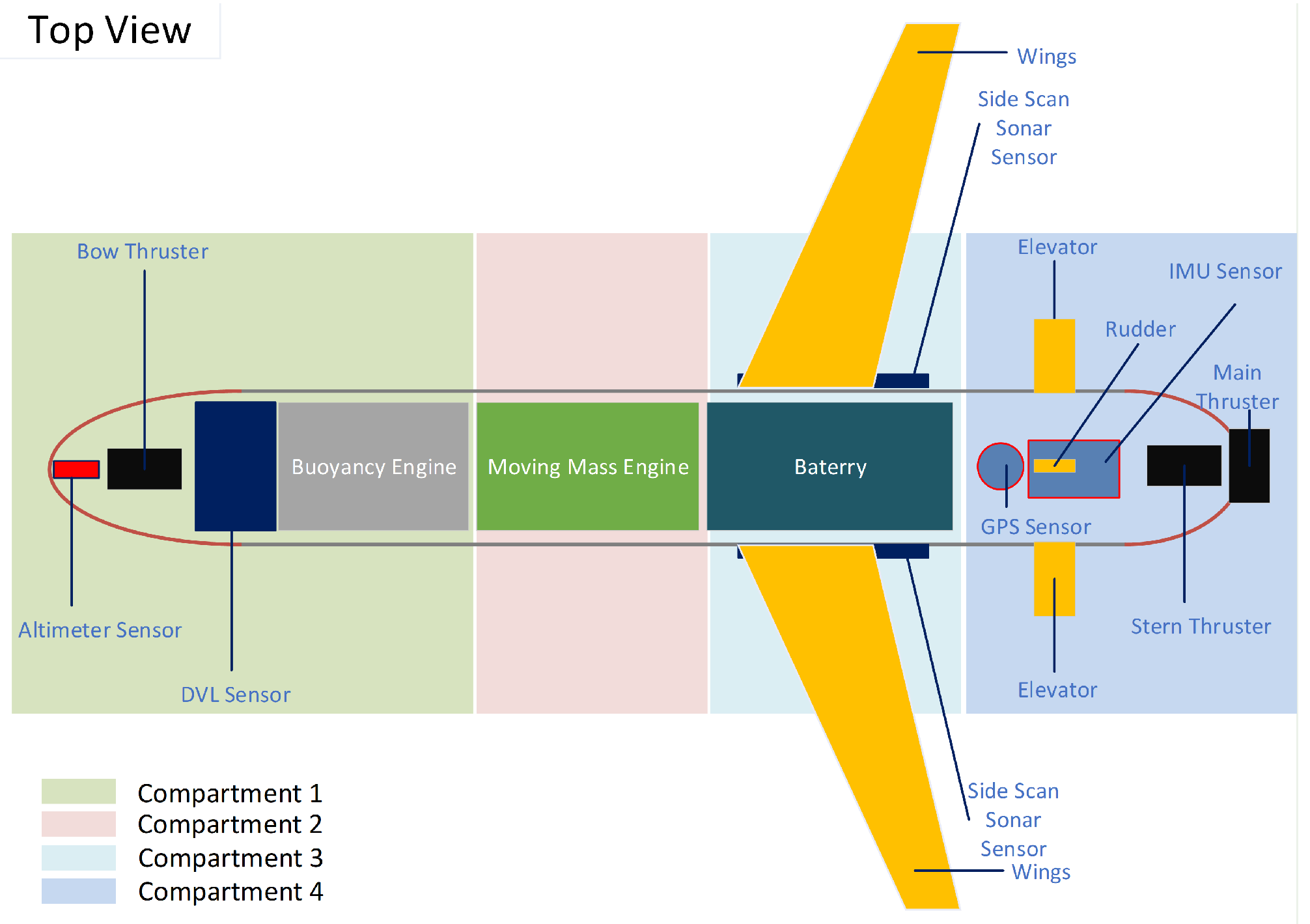
Figure 1.
HAUG’s concept design.
Figure 1.
HAUG’s concept design.
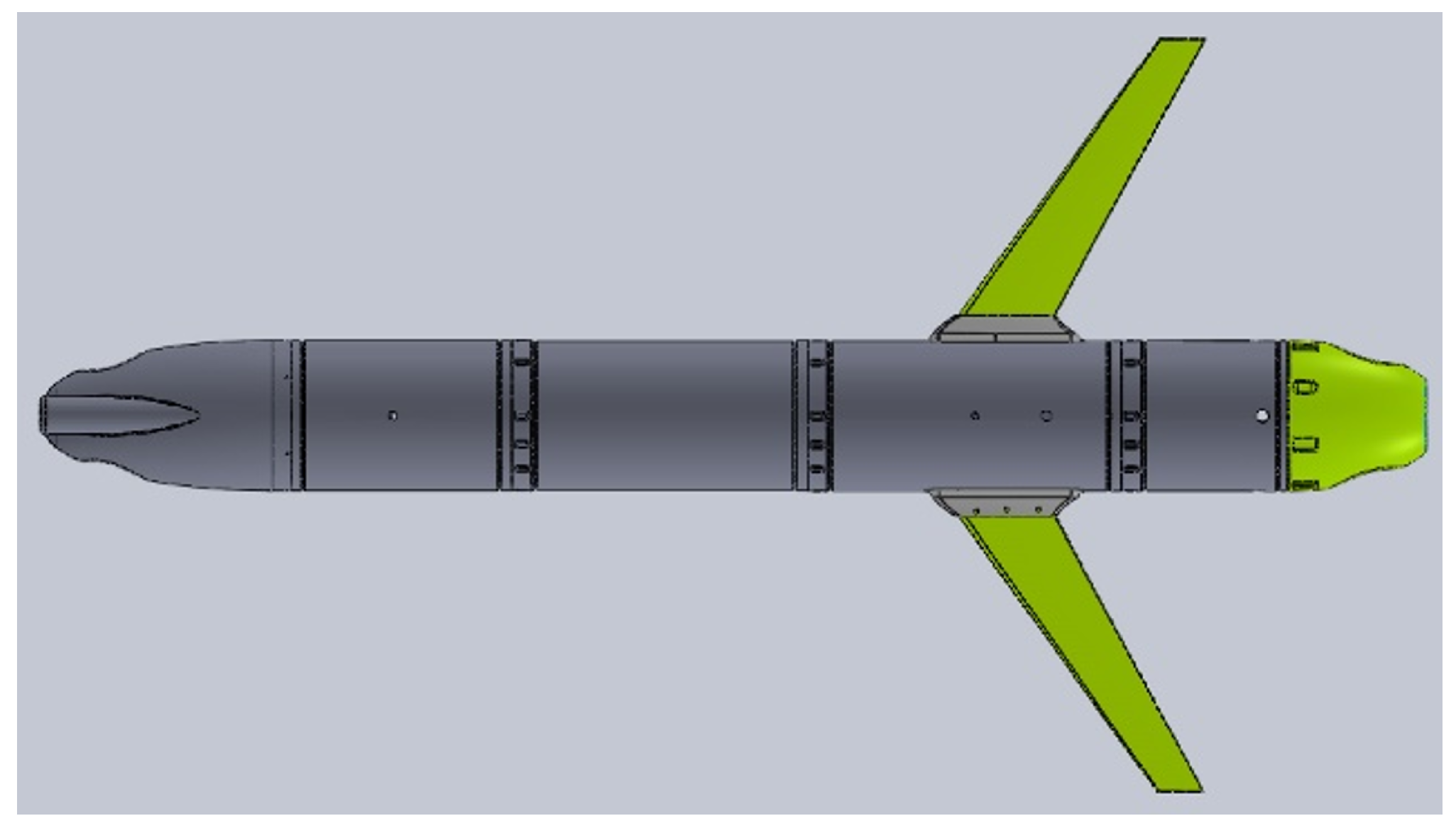
Figure 2.
Rendered concept design.
Figure 2.
Rendered concept design.
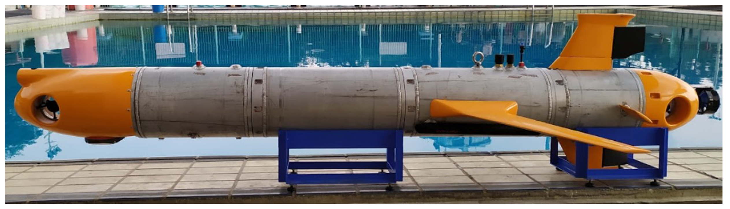
Figure 3.
Underwater HAUG prototype.
Figure 3.
Underwater HAUG prototype.
Figure 4.
Underwater HAUG’s buoyancy engine prototype.
Figure 4.
Underwater HAUG’s buoyancy engine prototype.
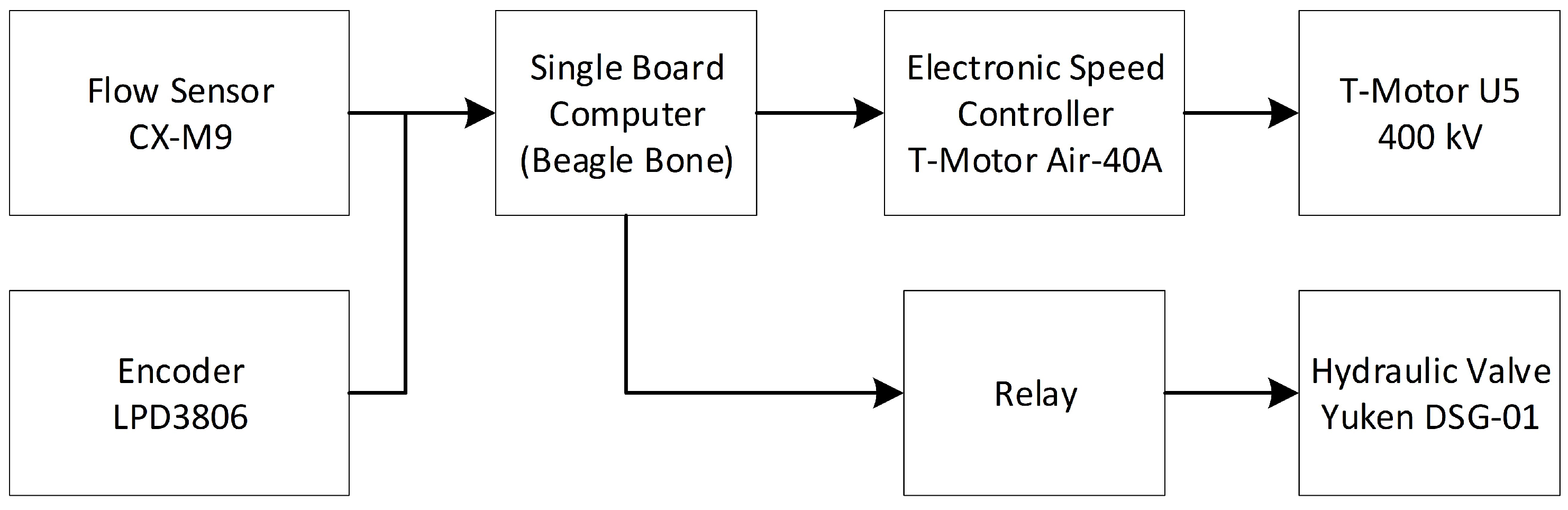
Figure 5.
Buoyancy engine block diagram.
Figure 5.
Buoyancy engine block diagram.
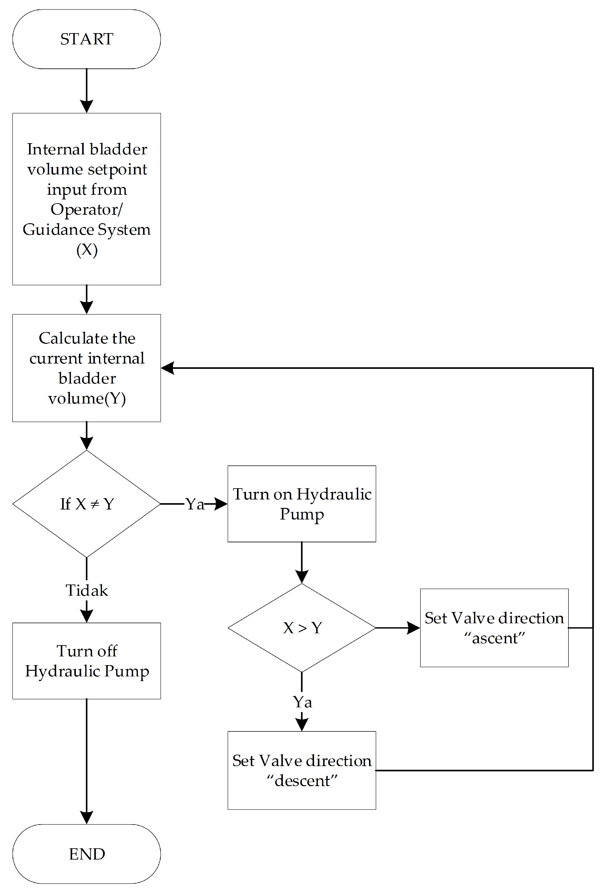
Figure 6.
Buoyancy engine workflow.
Figure 6.
Buoyancy engine workflow.
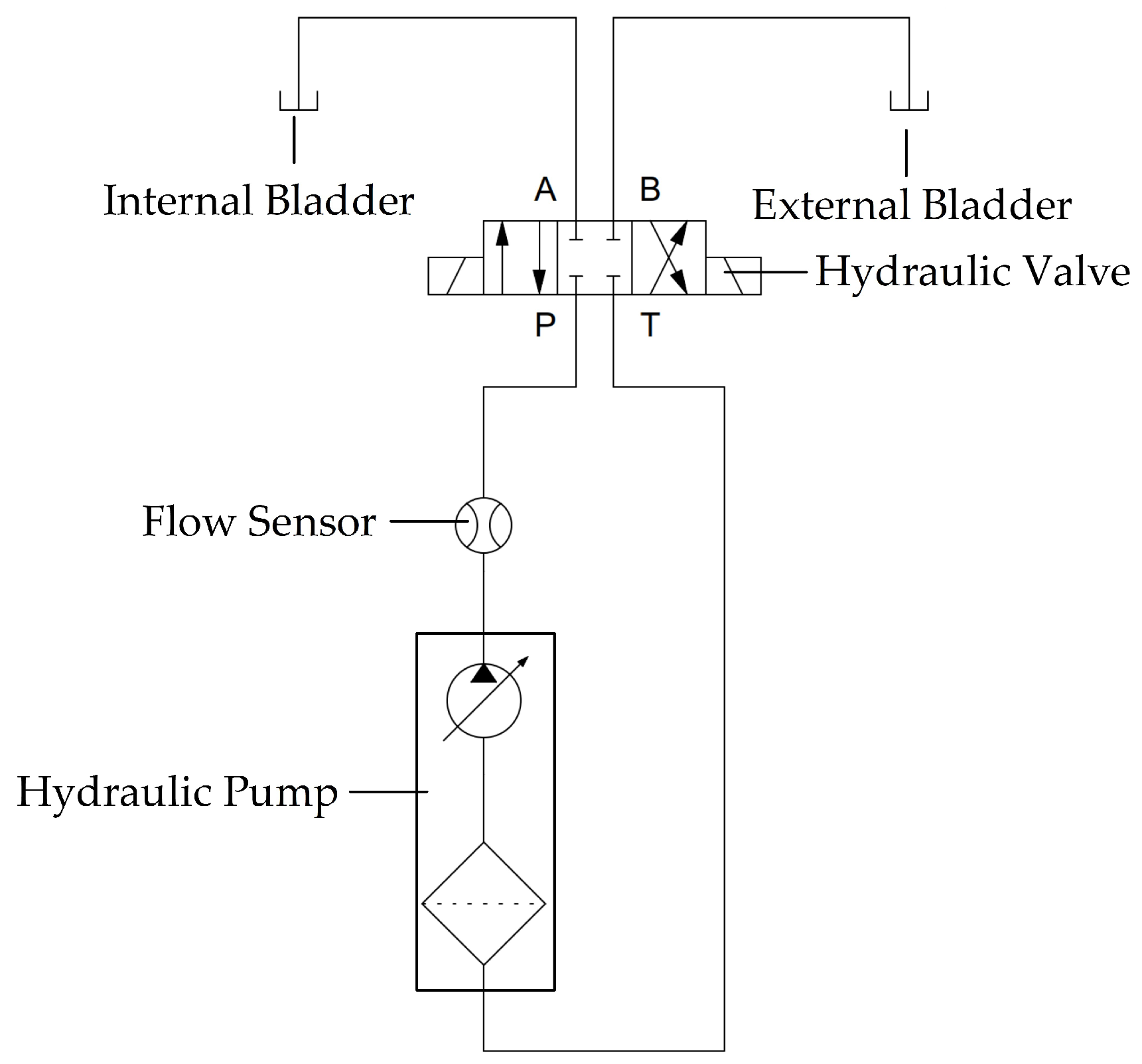
Figure 7.
Buoyancy engine’s hydraulic diagram.
Figure 7.
Buoyancy engine’s hydraulic diagram.
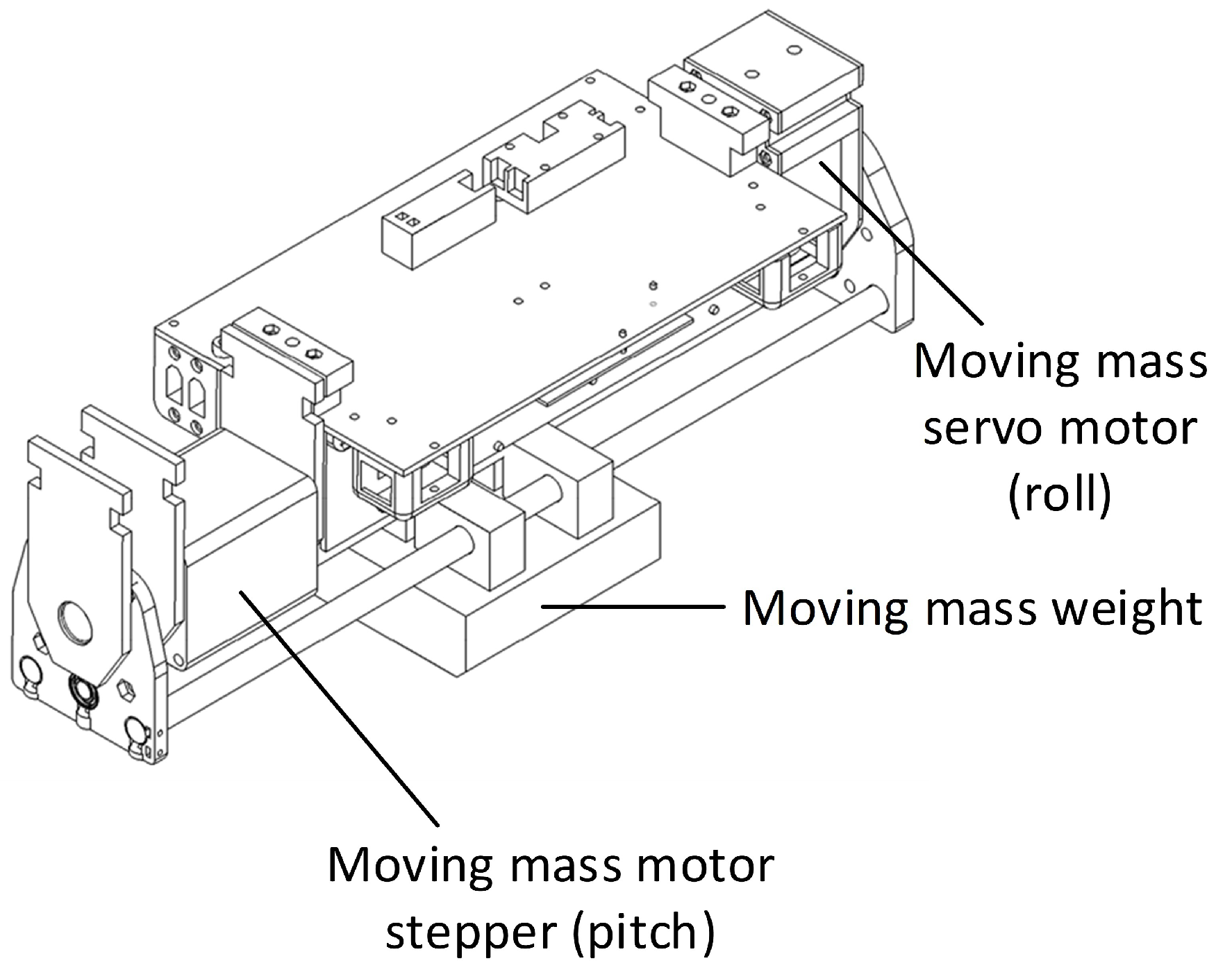
Figure 8.
Underwater HAUG’s moving-mass engine prototype.
Figure 8.
Underwater HAUG’s moving-mass engine prototype.
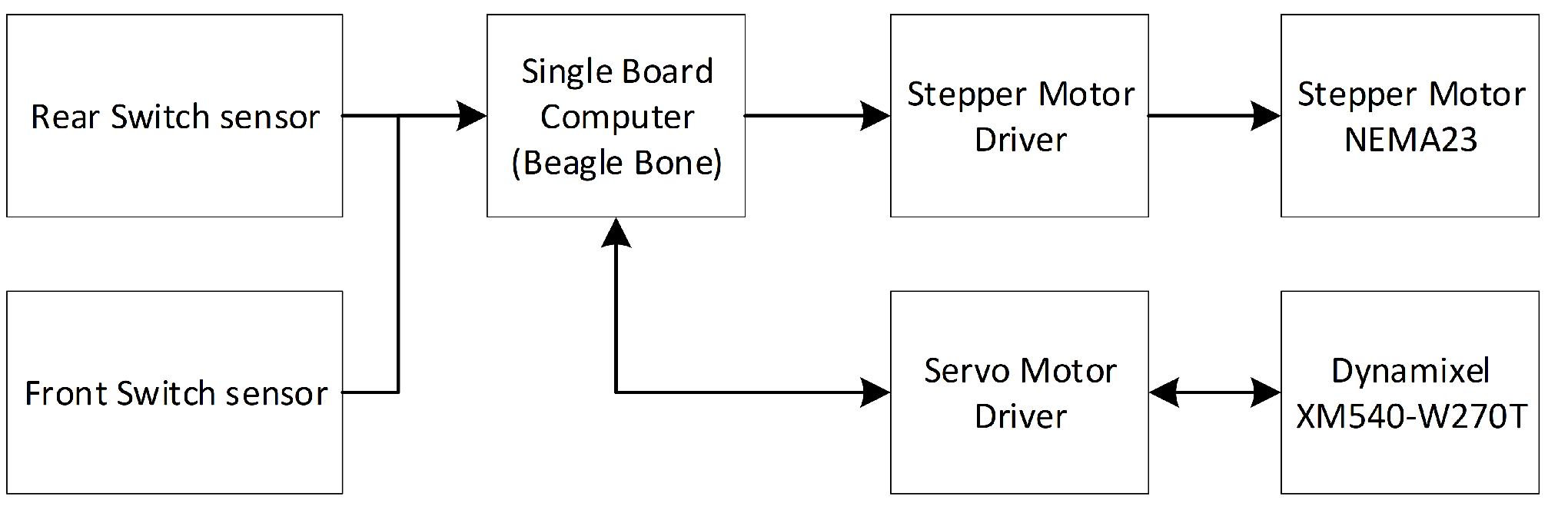
Figure 9.
Moving-mass engine block diagram.
Figure 9.
Moving-mass engine block diagram.
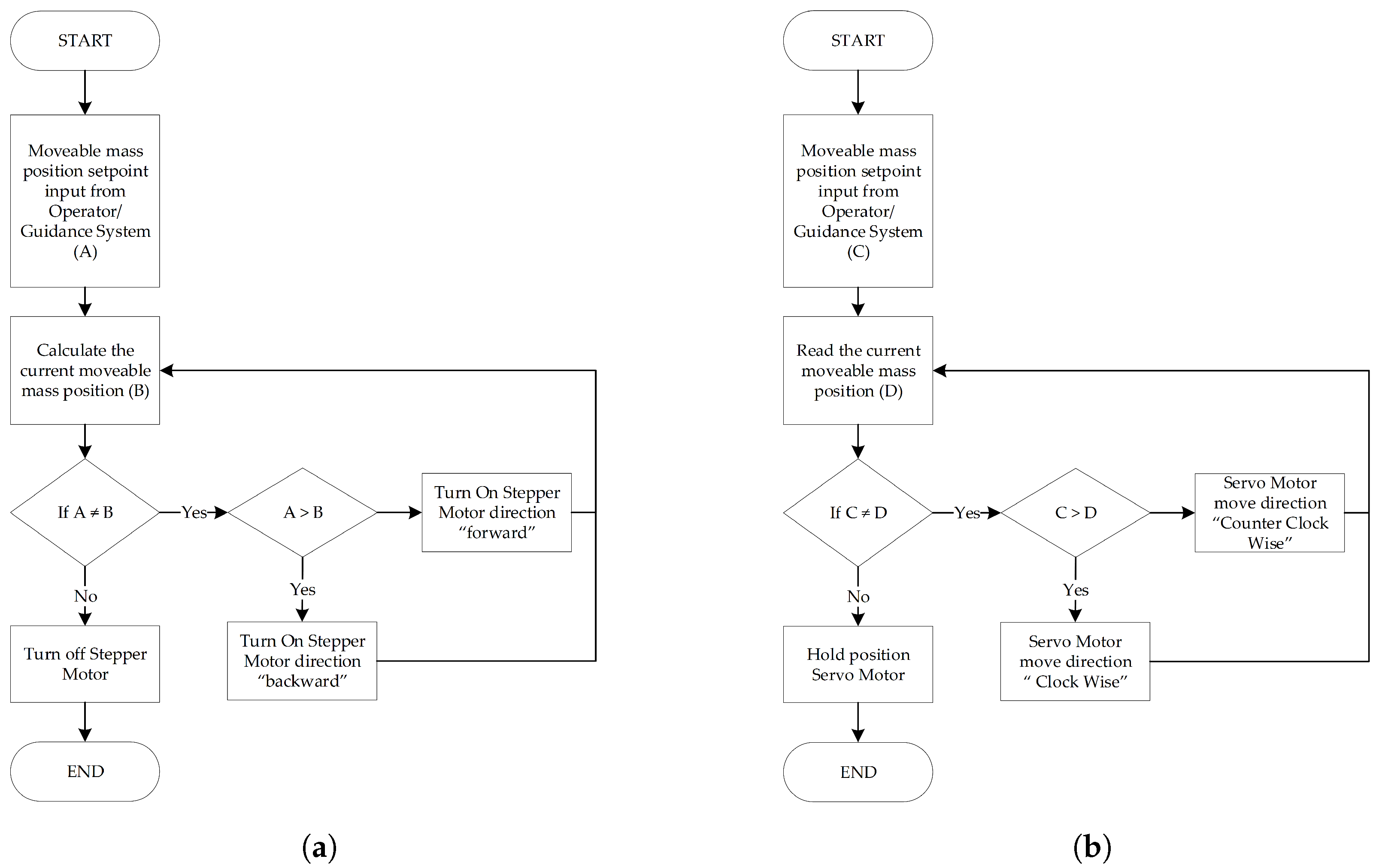
Figure 10.
Lateral and longitudinal engine workflow. (a) Moving mass’s pitch; (b) Moving mass’s roll.
Figure 10.
Lateral and longitudinal engine workflow. (a) Moving mass’s pitch; (b) Moving mass’s roll.
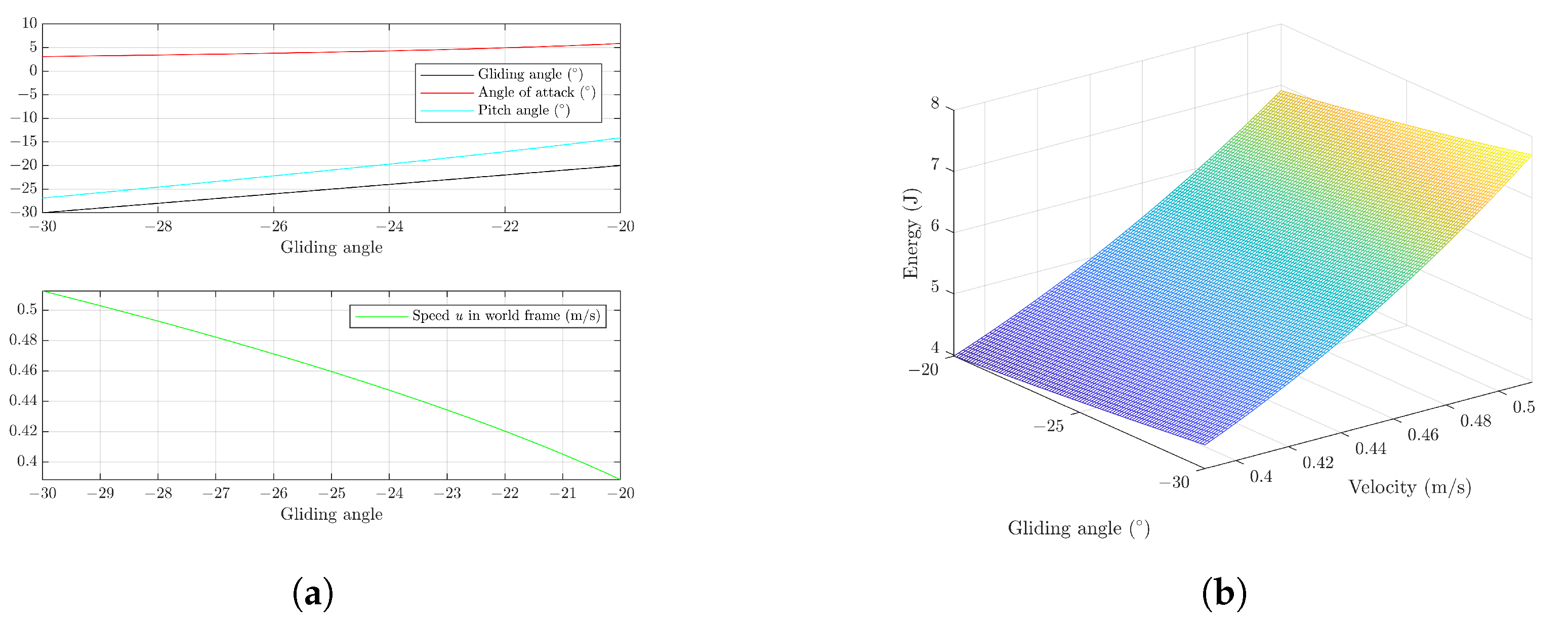
Figure 11.
Dynamicmodel simulation. (a) Gliding angle simulation; (b) mechanical energy, gliding angle, and velocity simulation.
Figure 11.
Dynamicmodel simulation. (a) Gliding angle simulation; (b) mechanical energy, gliding angle, and velocity simulation.
Figure 12.
Finite statemachine for underwater gliding motion.
Figure 12.
Finite statemachine for underwater gliding motion.
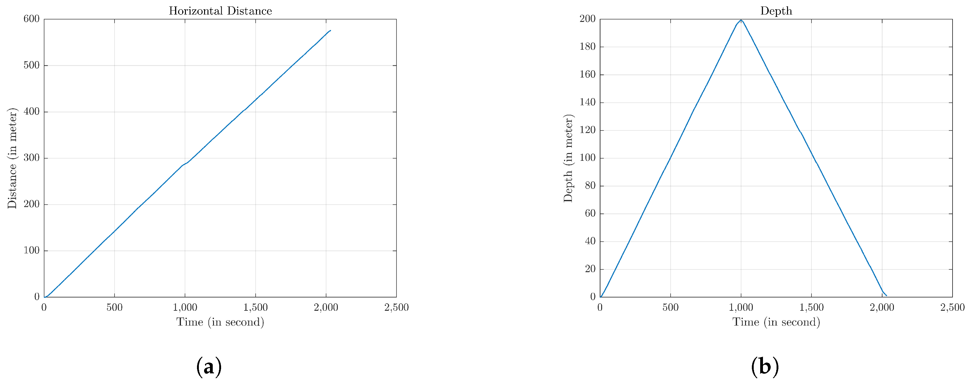
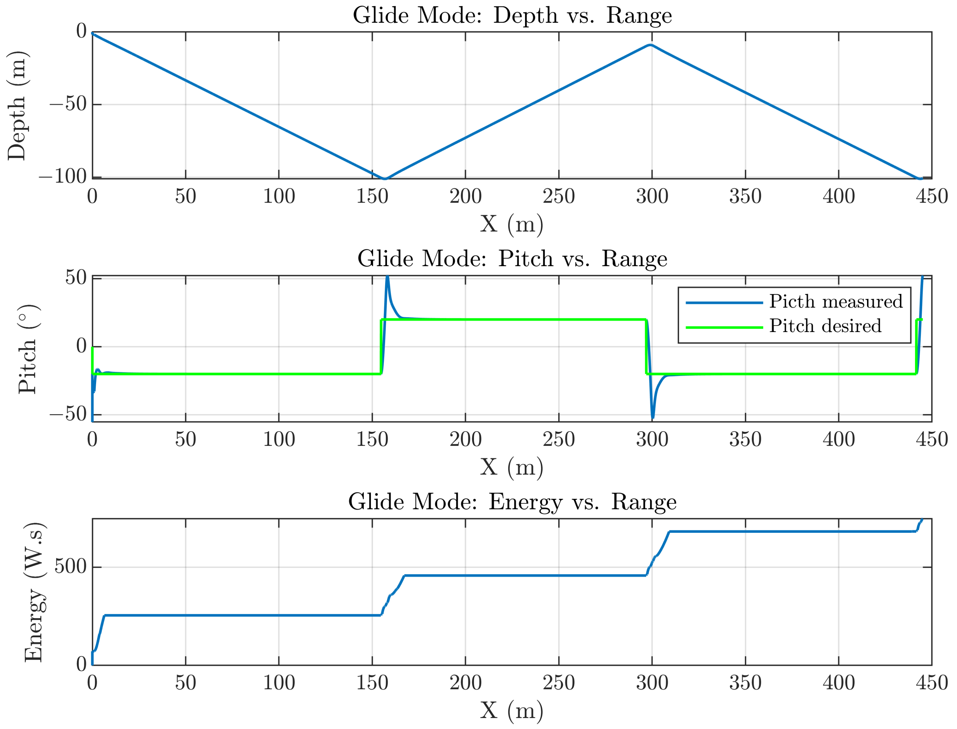
Figure 13.
Gliding motion simulation. (a) Simulation gliding motion in the distance axis; (b) simulation gliding motion in the depth axis.
Figure 13.
Gliding motion simulation. (a) Simulation gliding motion in the distance axis; (b) simulation gliding motion in the depth axis.
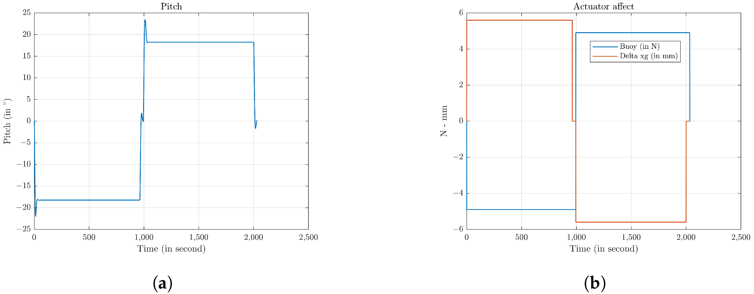
Figure 14.
Gliding motion simulation for pitch and actuator. (a) Simulation gliding motion with pitch axis; (b) the actuator motion in a gliding motion.
Figure 14.
Gliding motion simulation for pitch and actuator. (a) Simulation gliding motion with pitch axis; (b) the actuator motion in a gliding motion.
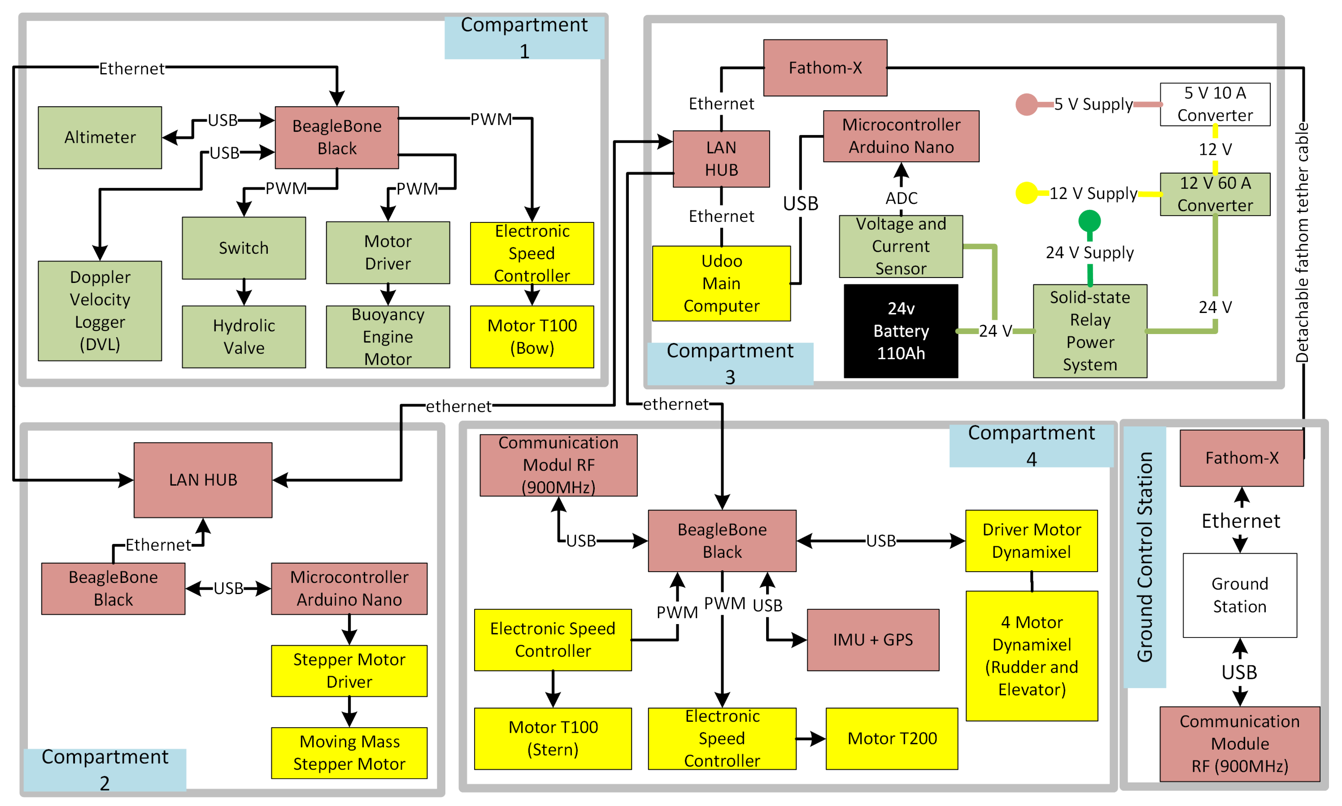
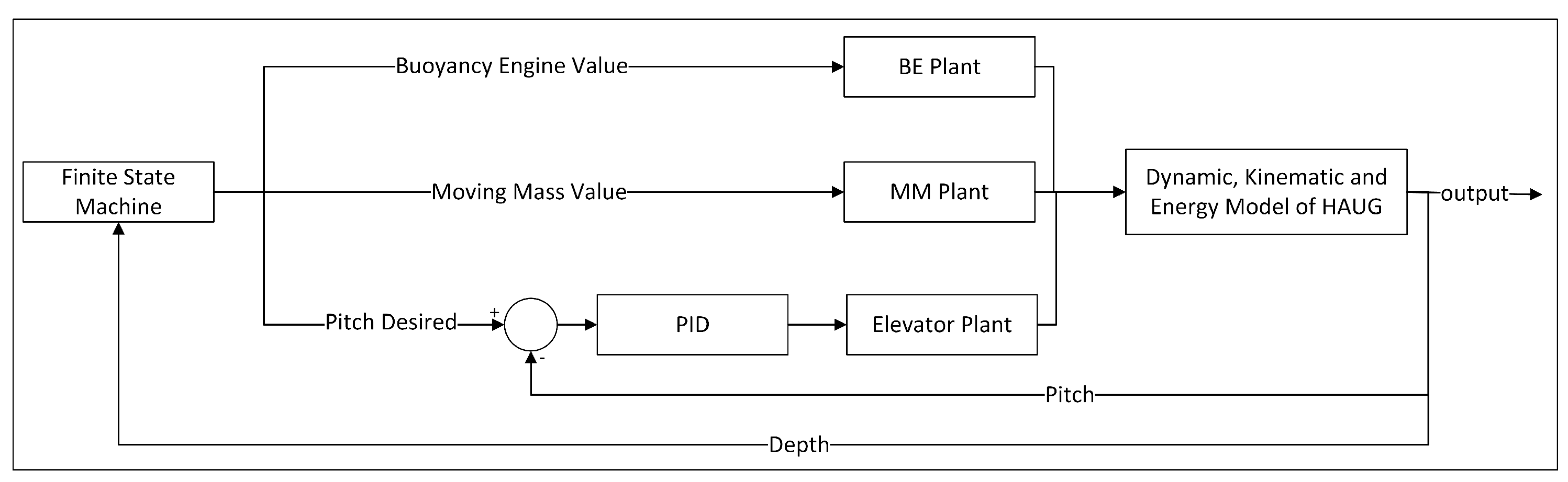
Figure 15.
Block diagram and electrical component of the HAUG.
Figure 15.
Block diagram and electrical component of the HAUG.
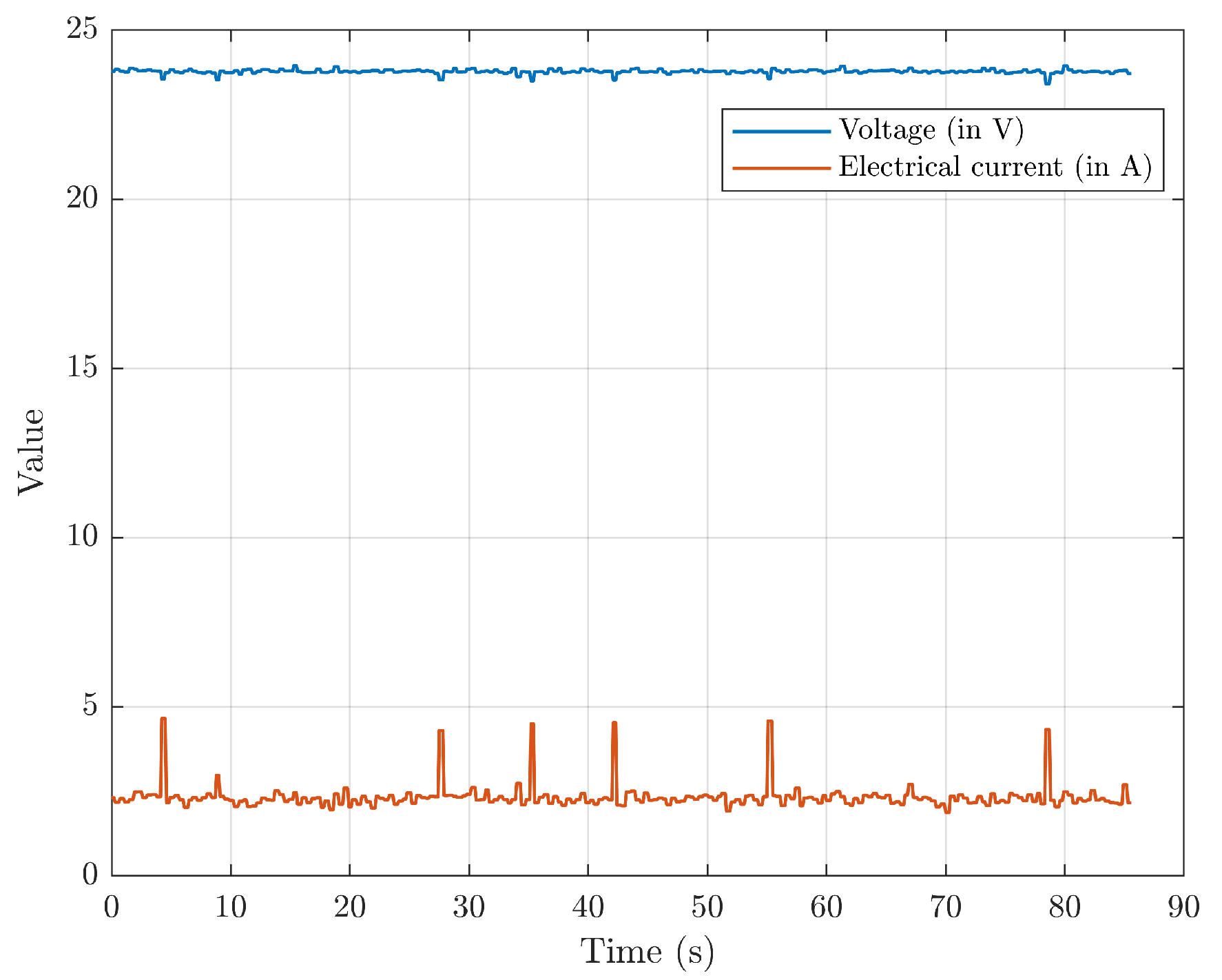
Figure 16.
The HAUG’s electrical power usage during the hotel load operation.
Figure 16.
The HAUG’s electrical power usage during the hotel load operation.
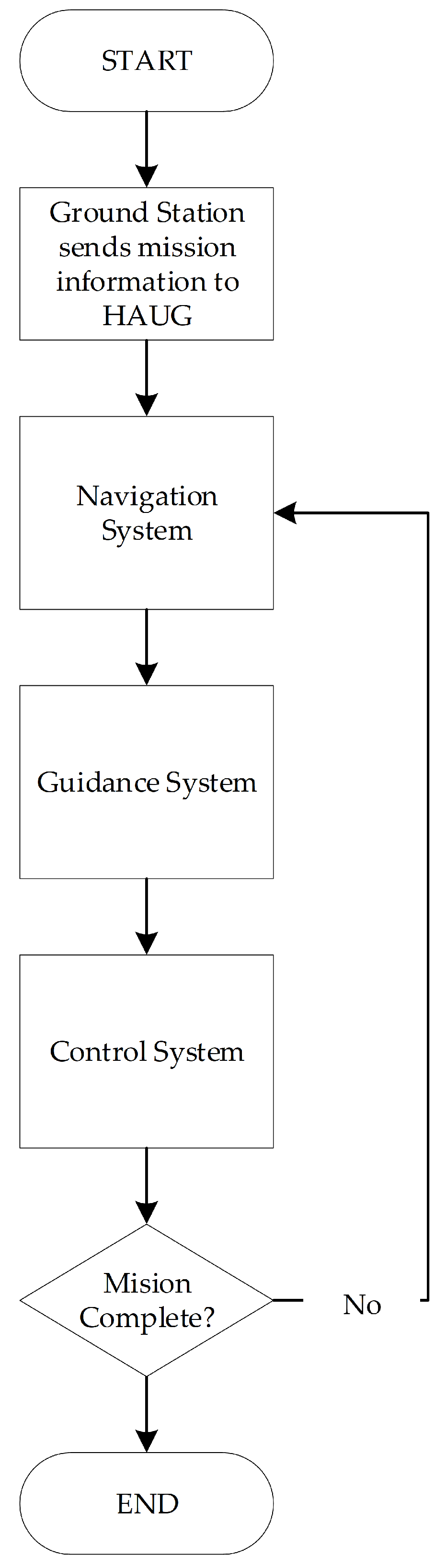
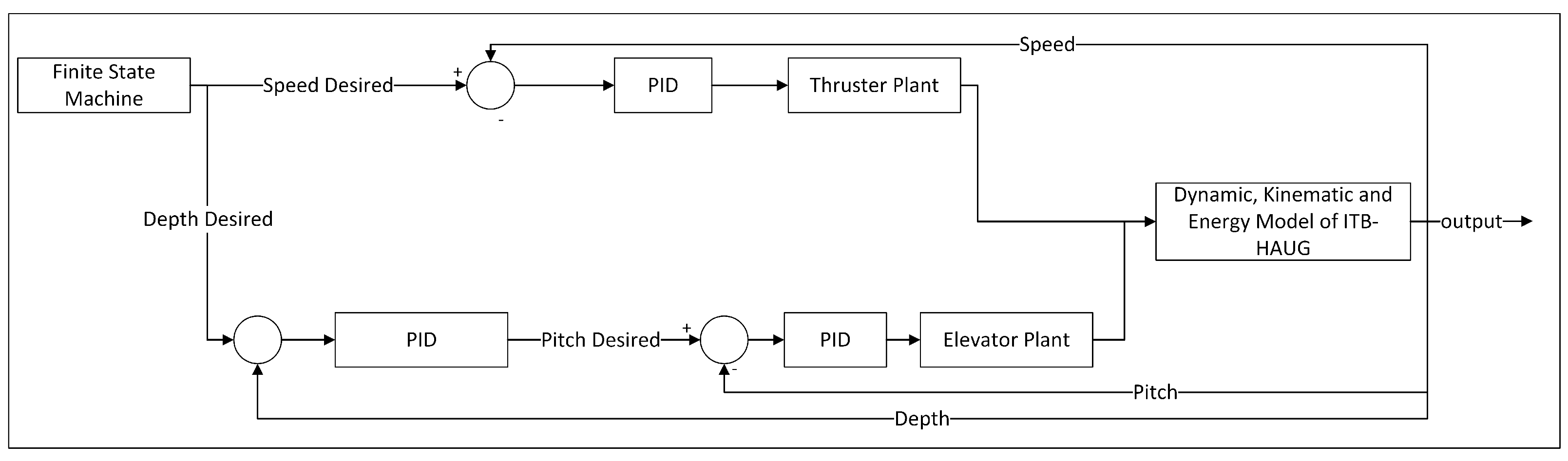
Figure 17.
Flowchart diagram of control system and guidance system.
Figure 17.
Flowchart diagram of control system and guidance system.
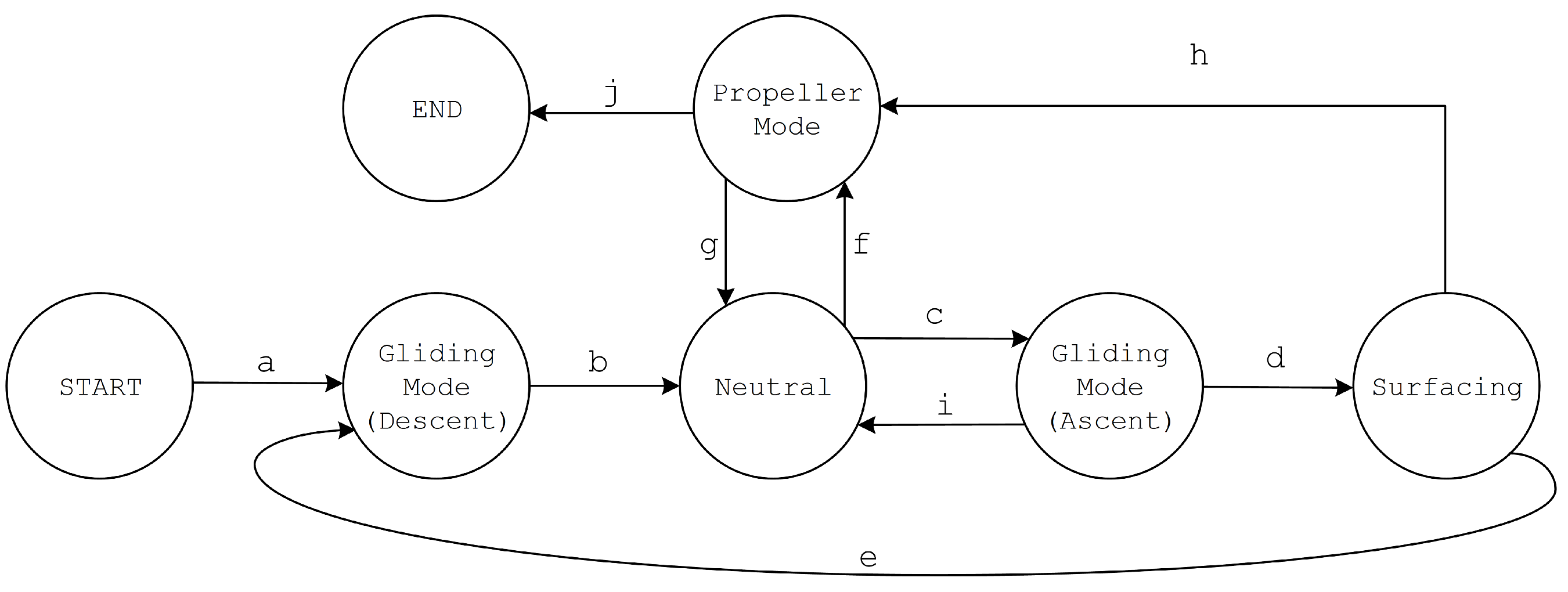
Figure 18.
Finite state machine of the HAUG.
Figure 18.
Finite state machine of the HAUG.
Figure 20.
The simulation resultof the buoyancy engine, moving mass, and pitch control.
Figure 20.
The simulation resultof the buoyancy engine, moving mass, and pitch control.
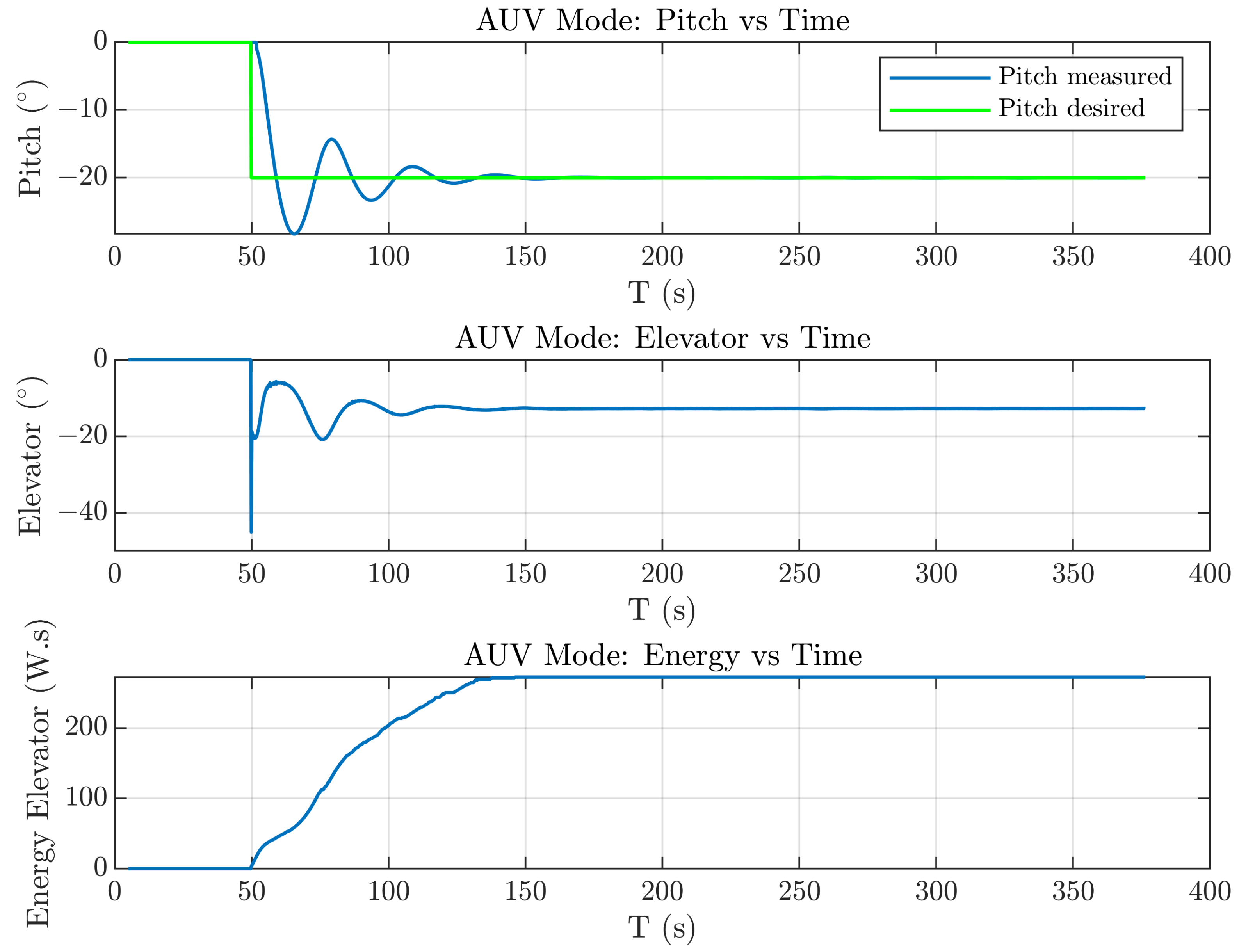
Figure 22.
Simulation results in AUV mode with the desired pitch.
Figure 22.
Simulation results in AUV mode with the desired pitch.
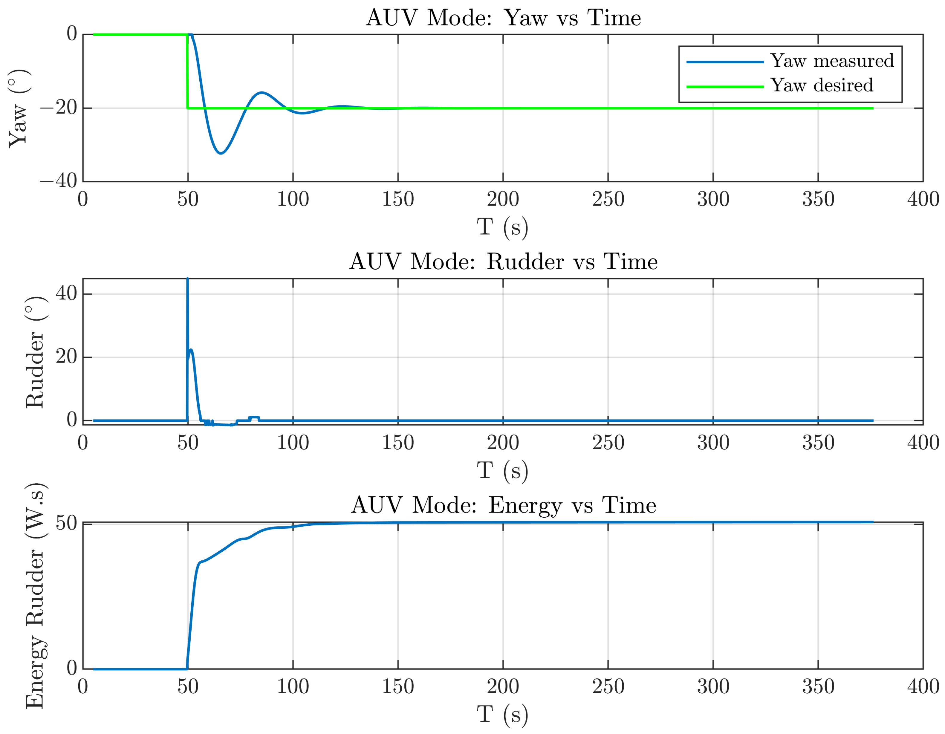
Figure 23.
Simulation results of AUV mode with the desired yaw.
Figure 23.
Simulation results of AUV mode with the desired yaw.
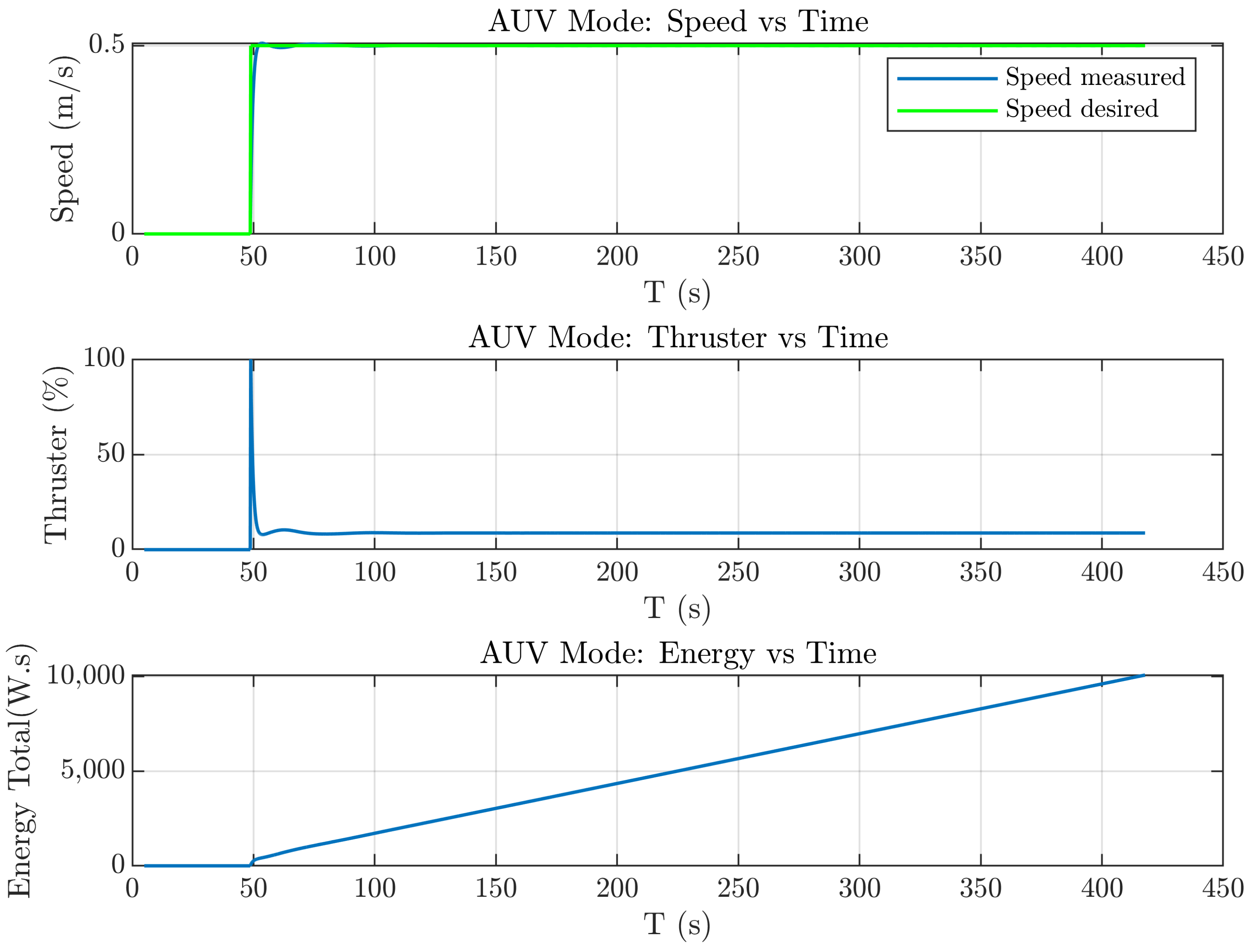
Figure 24.
Simulationresults of AUV mode with the desired speed.
Figure 24.
Simulationresults of AUV mode with the desired speed.
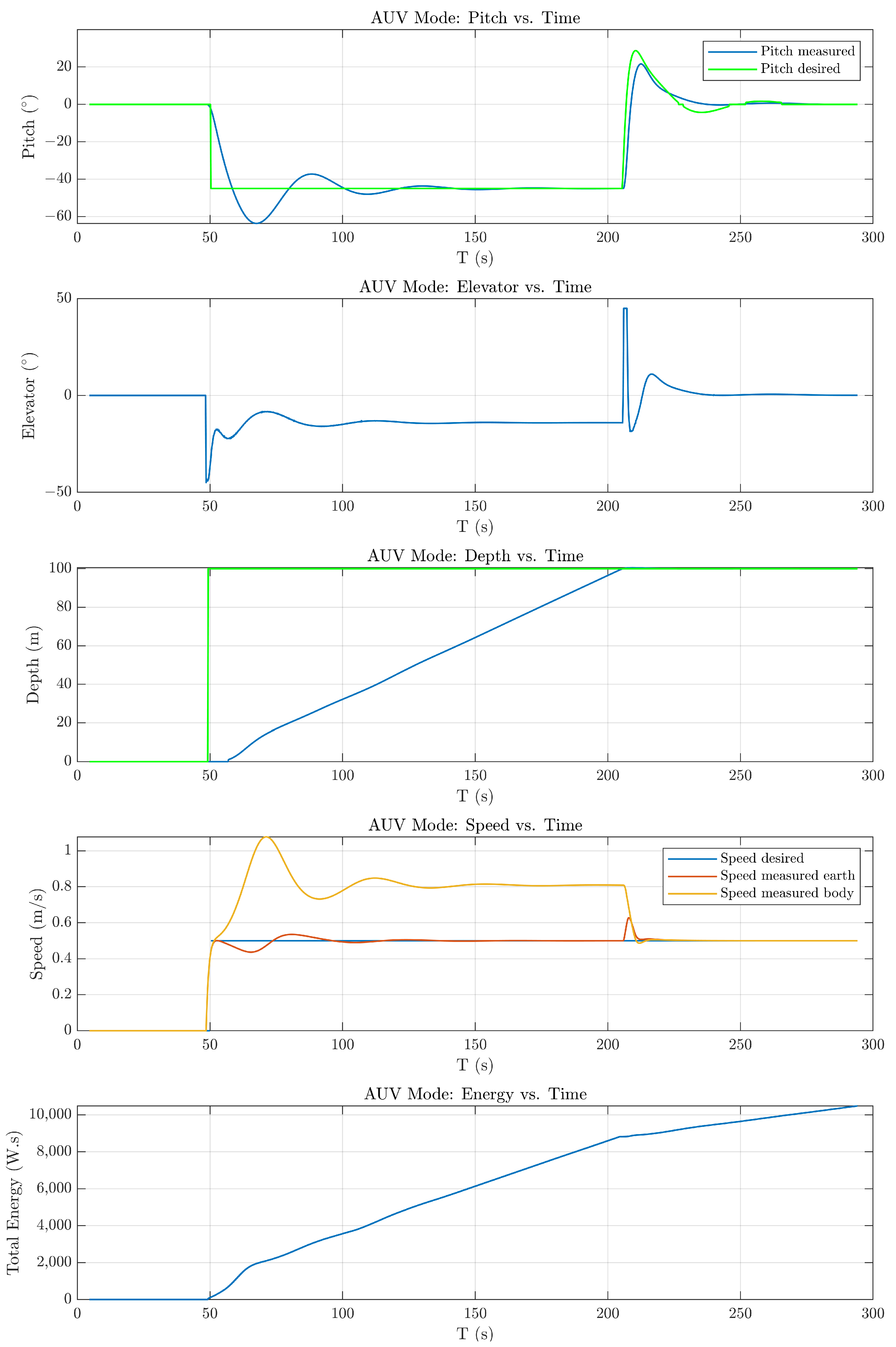
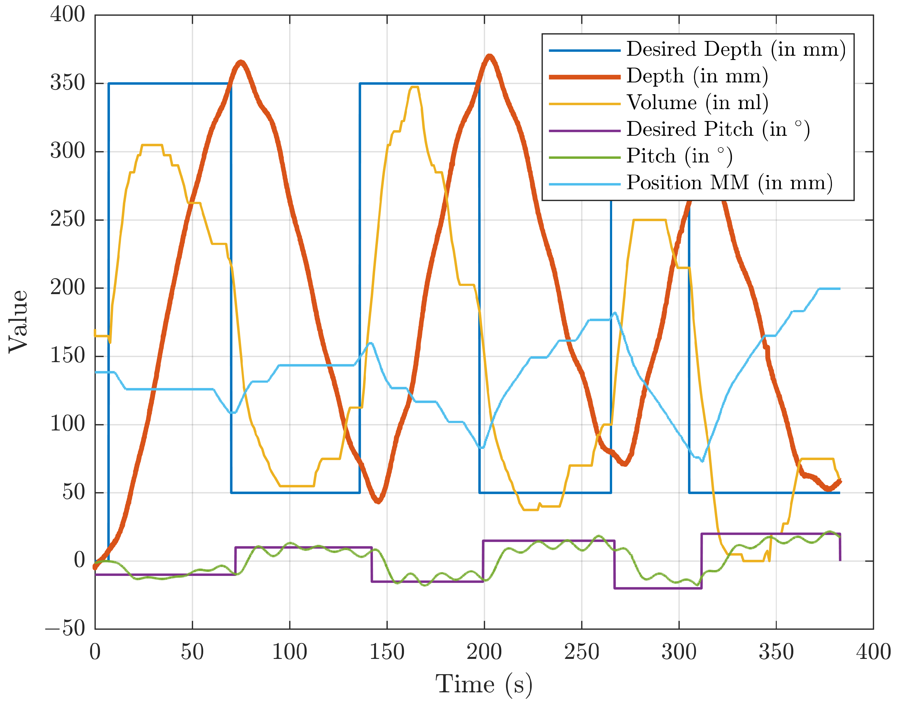
Figure 26.
The simulation resultsin AUV mode with desired speed and depth.
Figure 26.
The simulation resultsin AUV mode with desired speed and depth.
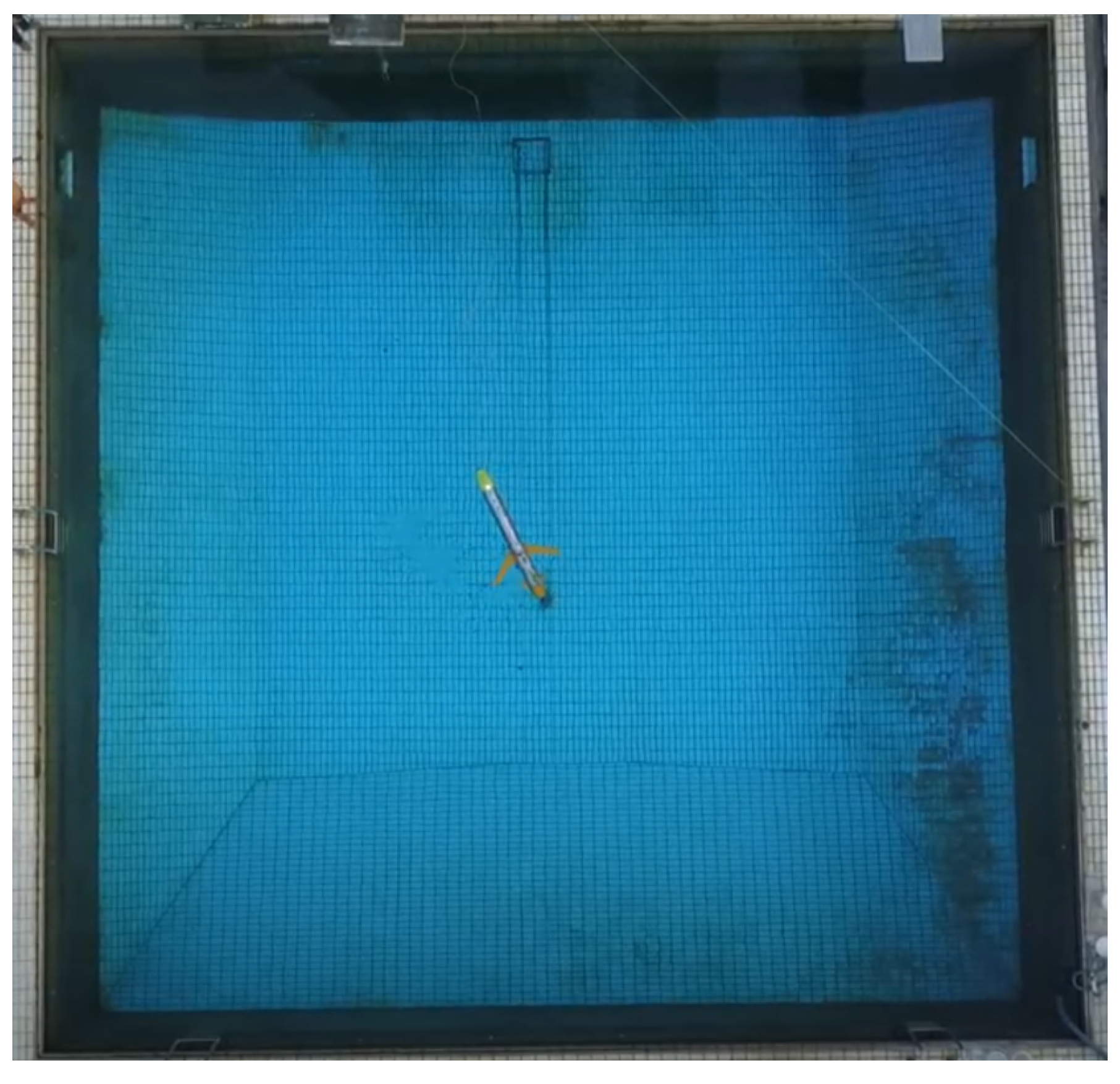
Figure 27.
The HAUG’s underwater experiment.
Figure 27.
The HAUG’s underwater experiment.
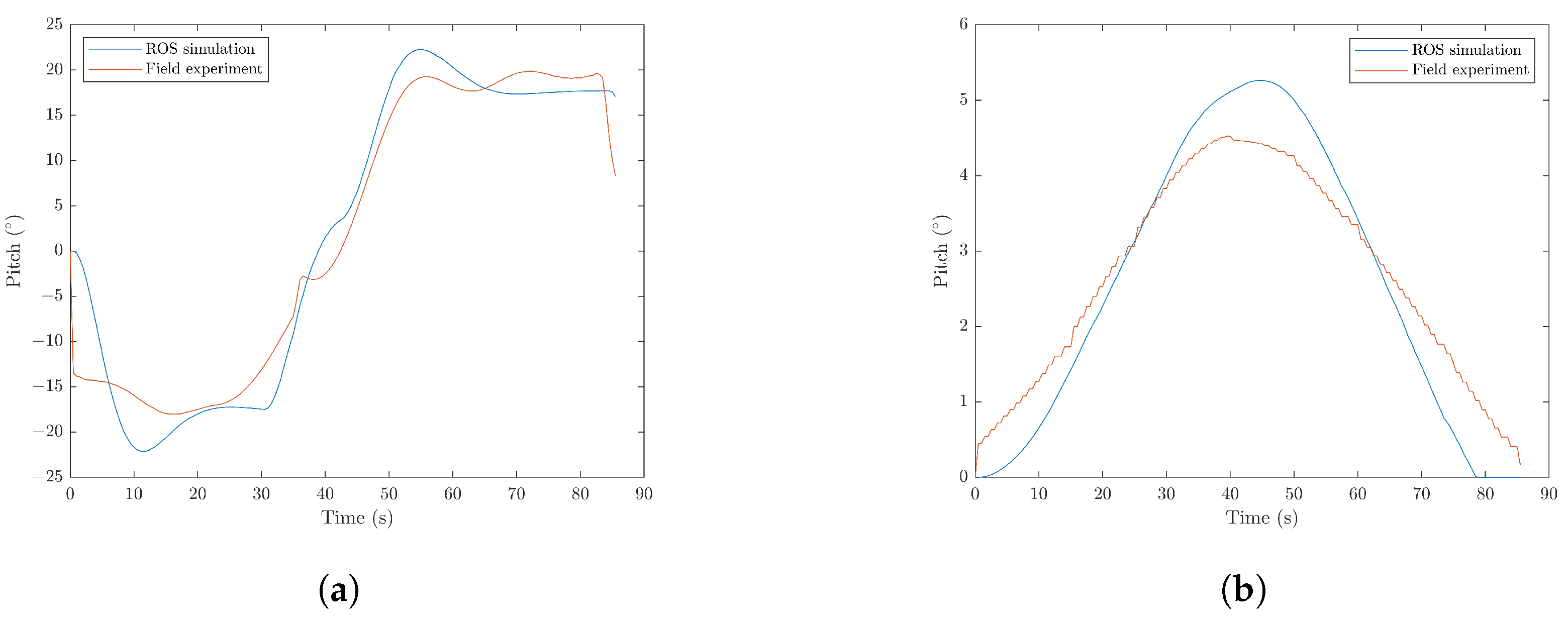
Figure 29.
ROS Simulation vs. field experiment result in Saraga’s swimming pool. (a) Pitch experiment; (b) depth experiment.
Figure 29.
ROS Simulation vs. field experiment result in Saraga’s swimming pool. (a) Pitch experiment; (b) depth experiment.
Figure 30.
Moving- mass and buoyancy engine performance in gliding mode.
Figure 30.
Moving- mass and buoyancy engine performance in gliding mode.
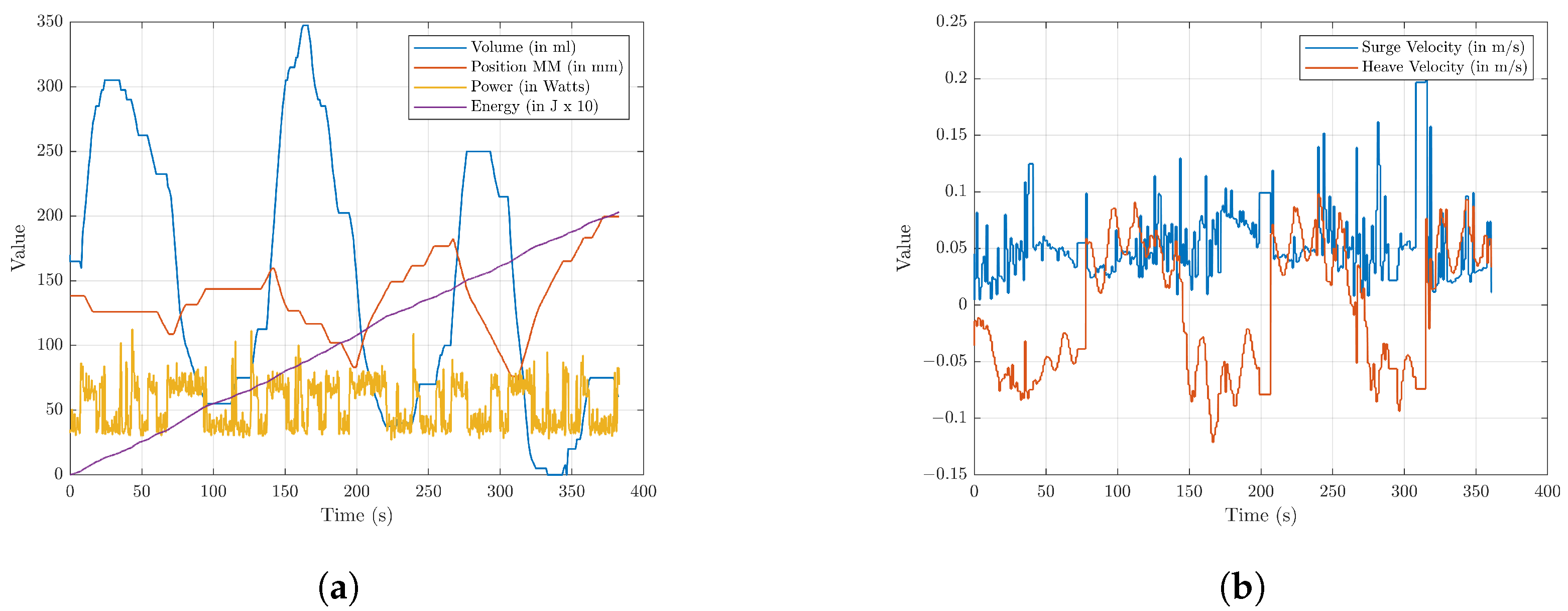
Figure 31.
Energy consumption and velocity measurement in 3 gliding cycles. (a) Energy consumption; (b) surge and heave velocity.
Figure 31.
Energy consumption and velocity measurement in 3 gliding cycles. (a) Energy consumption; (b) surge and heave velocity.
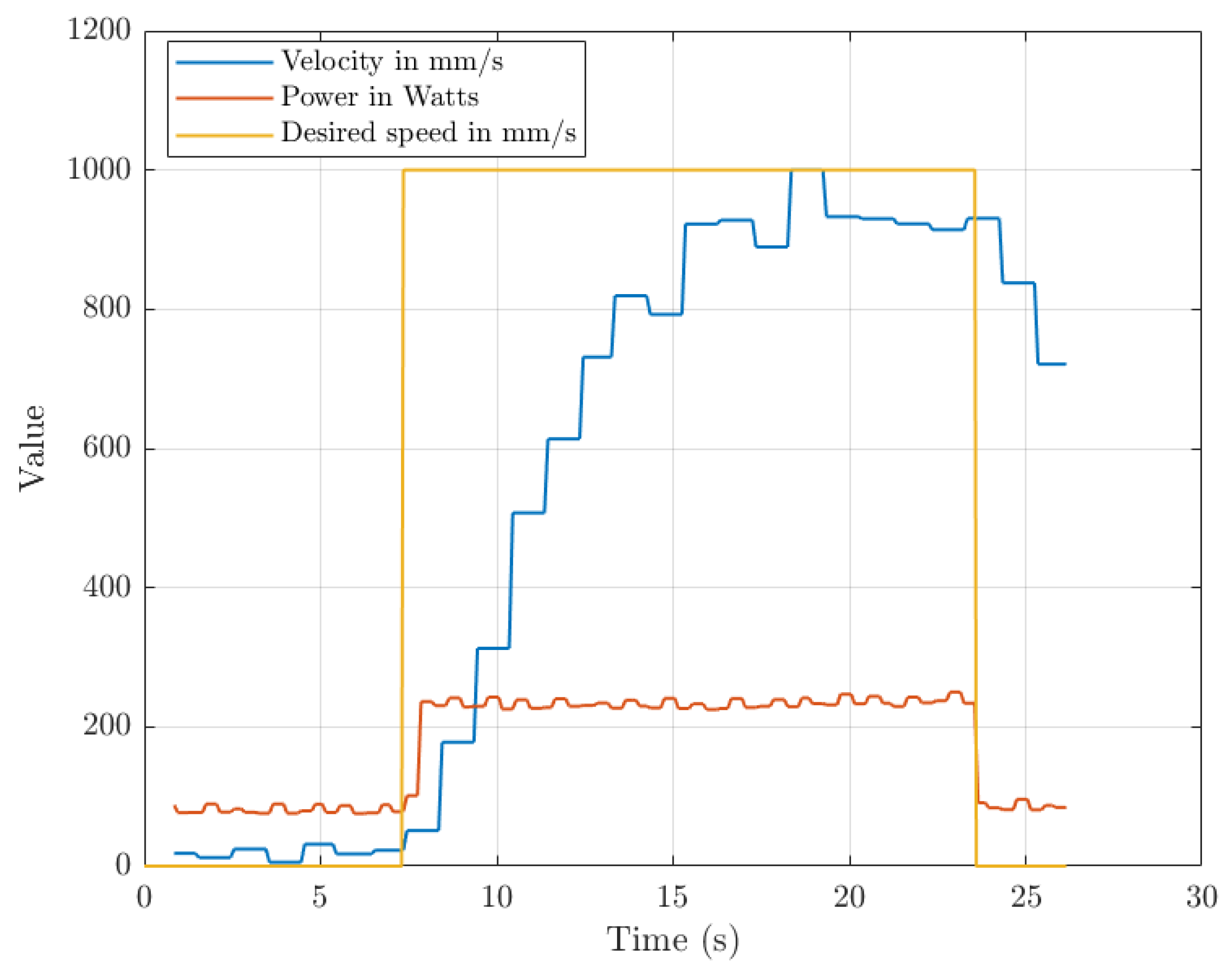
Figure 32.
Energy and velocity measurement in AUV mode.
Figure 32.
Energy and velocity measurement in AUV mode.
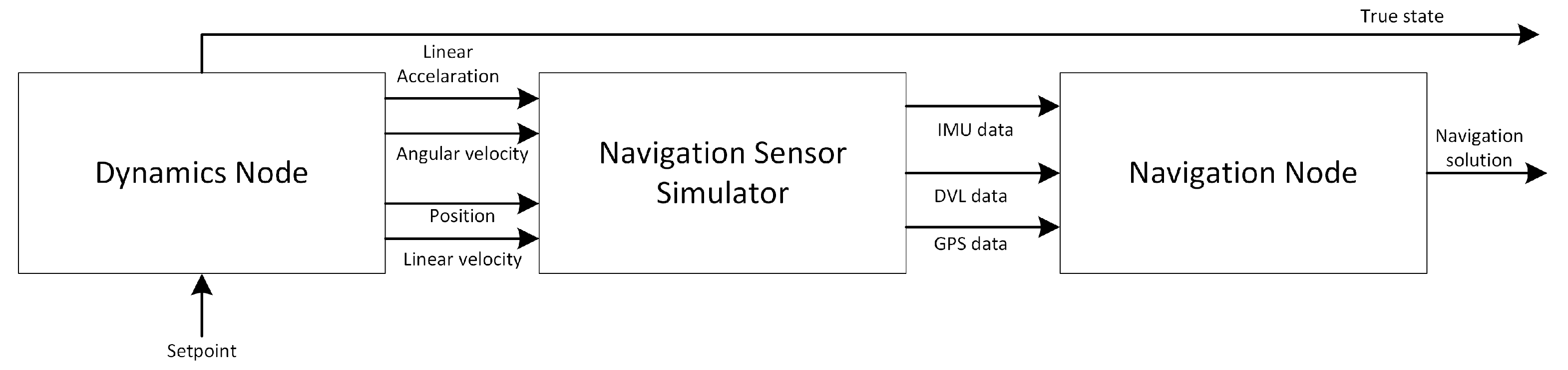
Figure 33.
The HAUG’s navigation system simulation design.
Figure 33.
The HAUG’s navigation system simulation design.
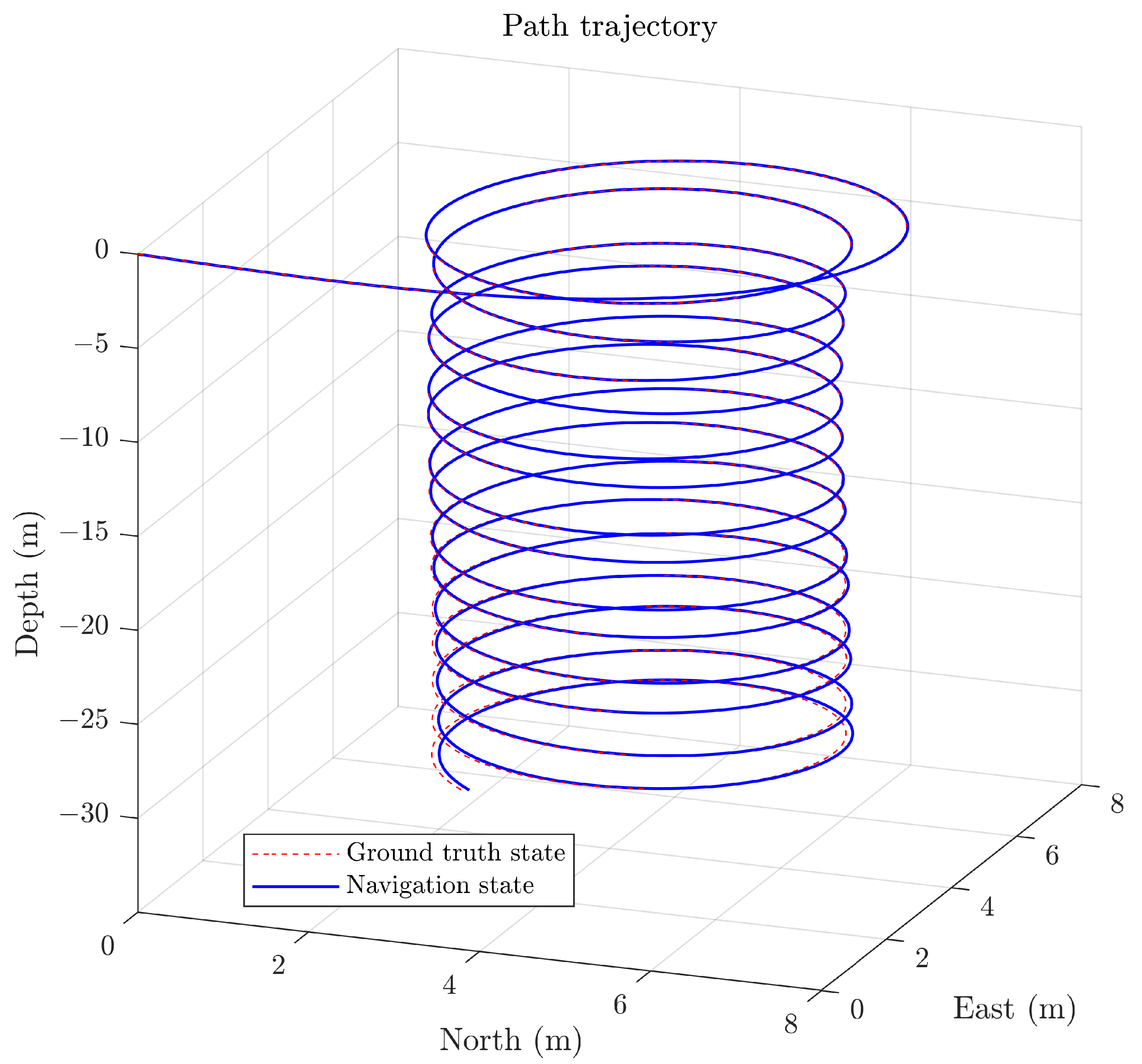
Figure 34.
Three-dimensional helix moving simulation.
Figure 34.
Three-dimensional helix moving simulation.
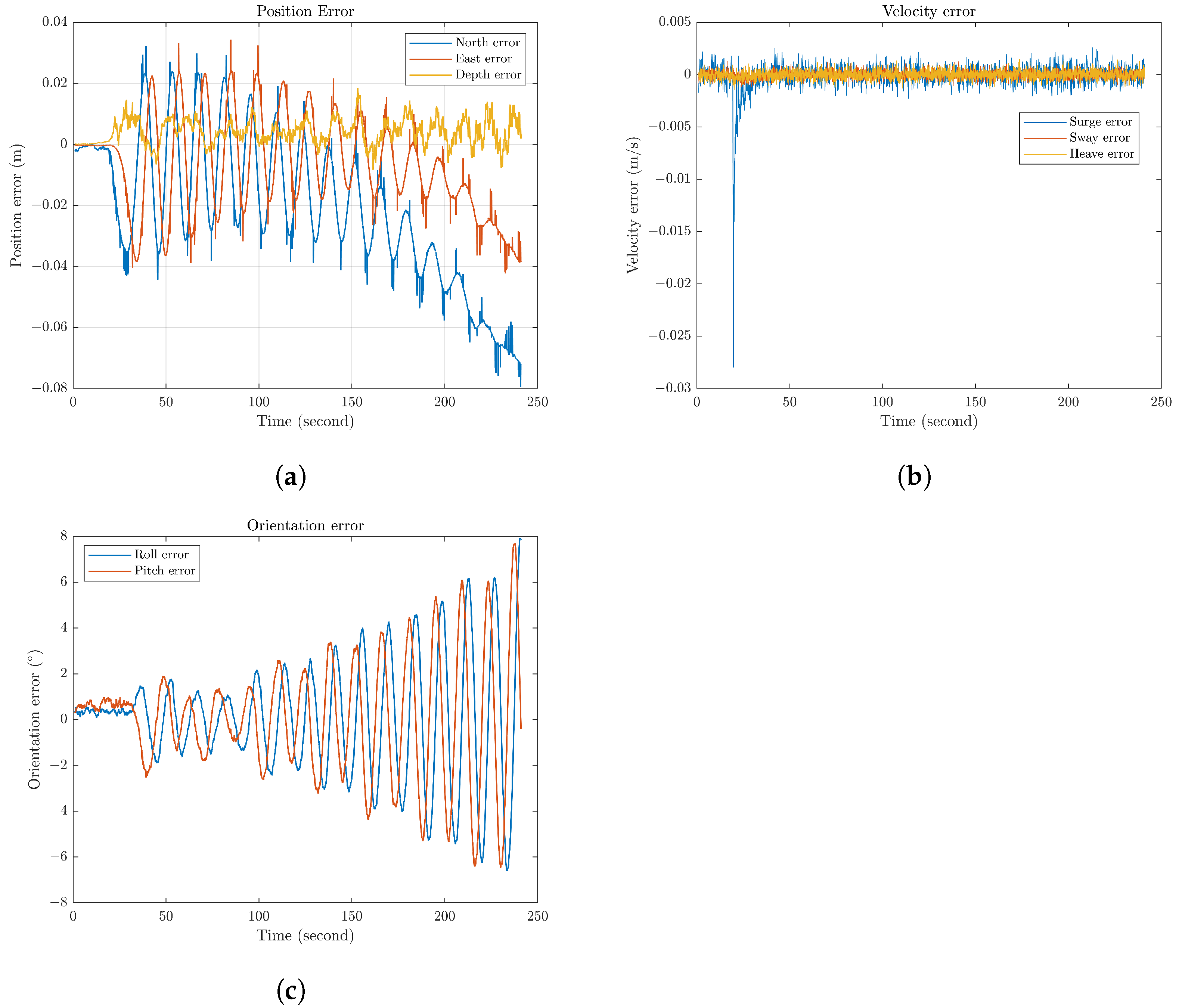
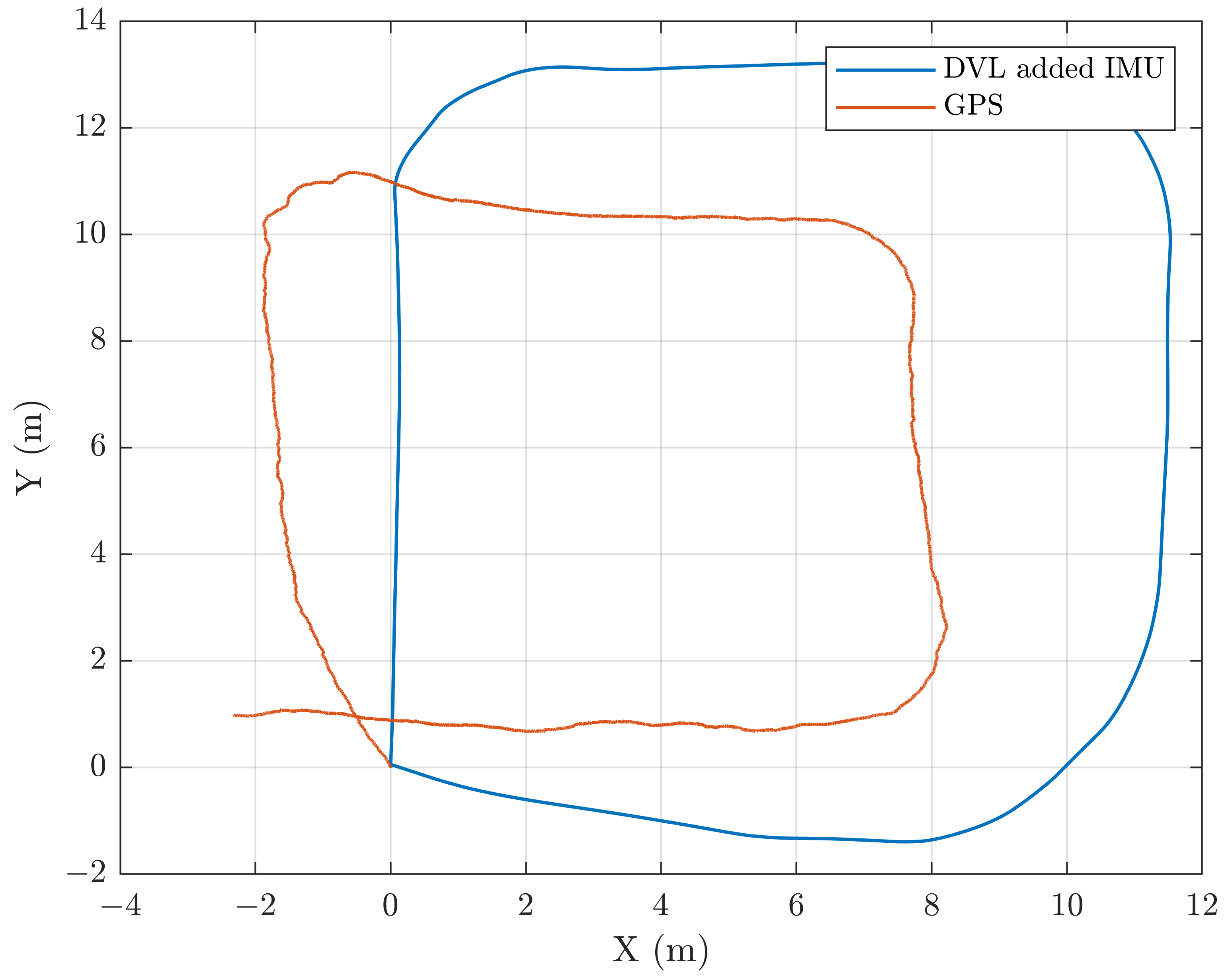
Figure 35.
Three-dimensional Helix motion error. (a) Position error; (b) velocity error; (c) orientation error.
Figure 35.
Three-dimensional Helix motion error. (a) Position error; (b) velocity error; (c) orientation error.
Figure 36.
Saraga’s ITB Diving Pool.
Figure 36.
Saraga’s ITB Diving Pool.
Figure 37.
Rotational motion scenario for the yaw experiment using the stern thruster. (a) Thruster output and IMU sensor; (b) Yaw simulation and field experiment.
Figure 37.
Rotational motion scenario for the yaw experiment using the stern thruster. (a) Thruster output and IMU sensor; (b) Yaw simulation and field experiment.
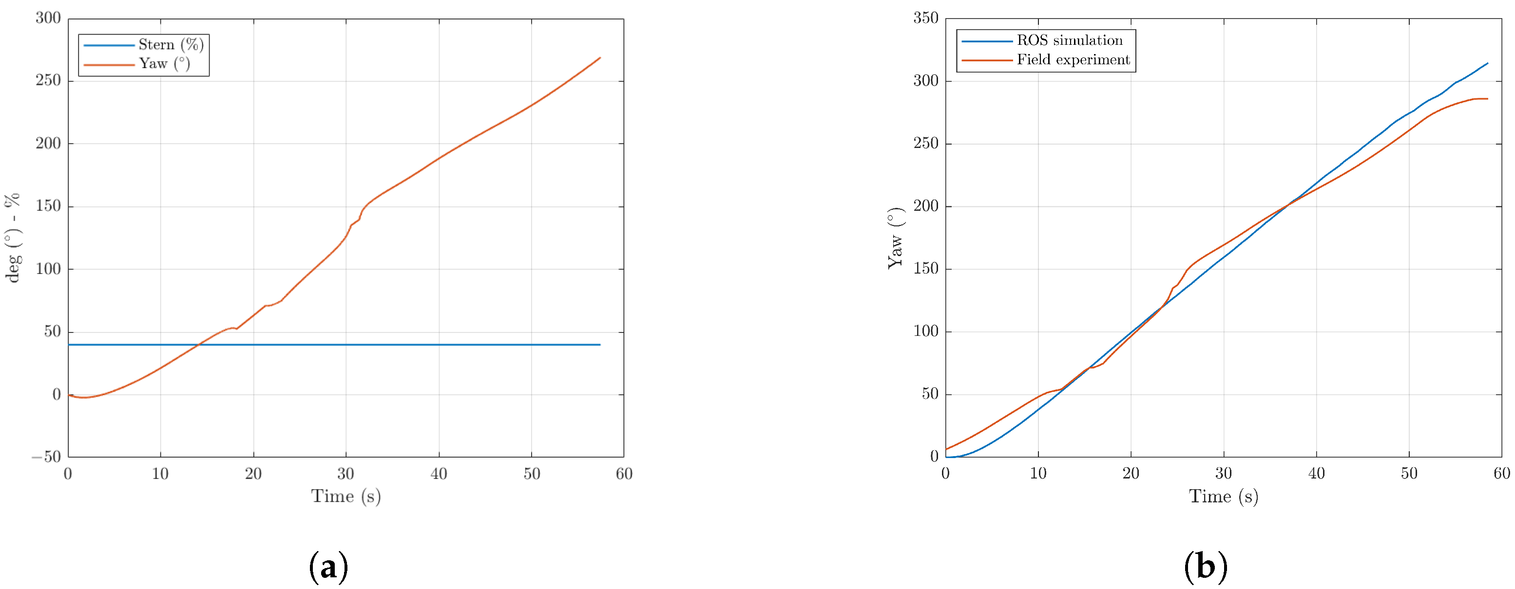
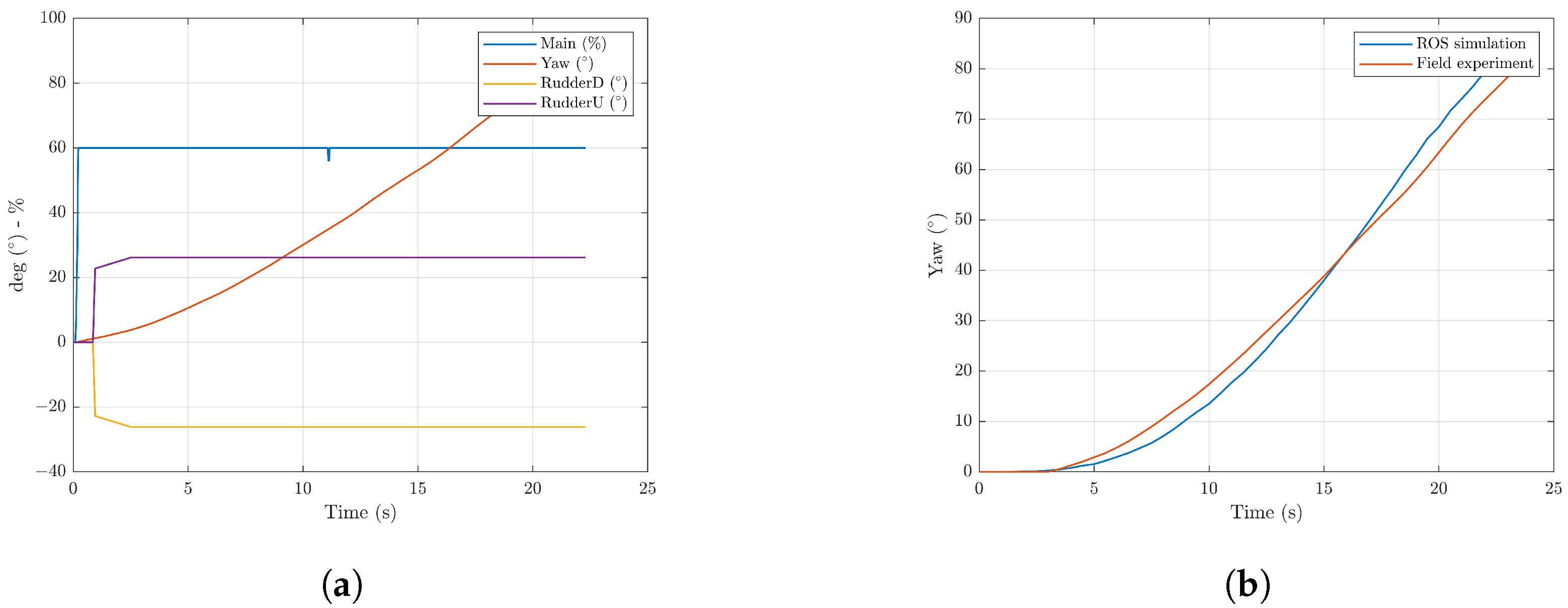
Figure 38.
Rotational motion scenario for the yaw experiment based on the IMU using the main thruster and rudder. (a) Thruster–rudder output and IMU sensor; (b) Yaw simulation and field experiment.
Figure 38.
Rotational motion scenario for the yaw experiment based on the IMU using the main thruster and rudder. (a) Thruster–rudder output and IMU sensor; (b) Yaw simulation and field experiment.
Figure 39.
Rectangular motion around the pool scenario.
Figure 39.
Rectangular motion around the pool scenario.
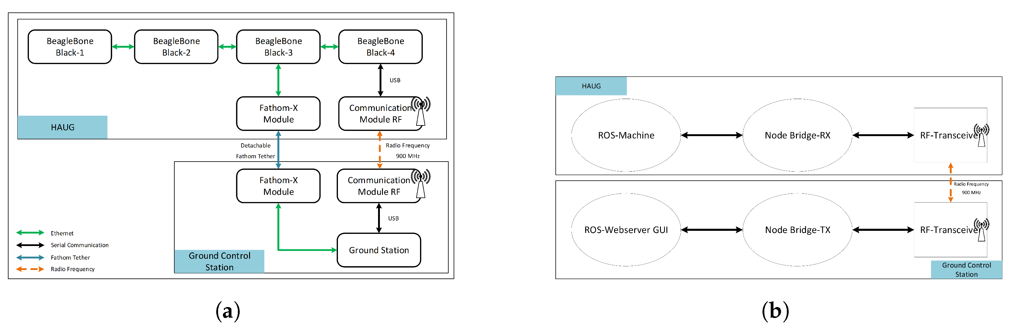
Figure 40.
Communication system design. (a) Communication system diagram block; (b) ROS node communication design.
Figure 40.
Communication system design. (a) Communication system diagram block; (b) ROS node communication design.
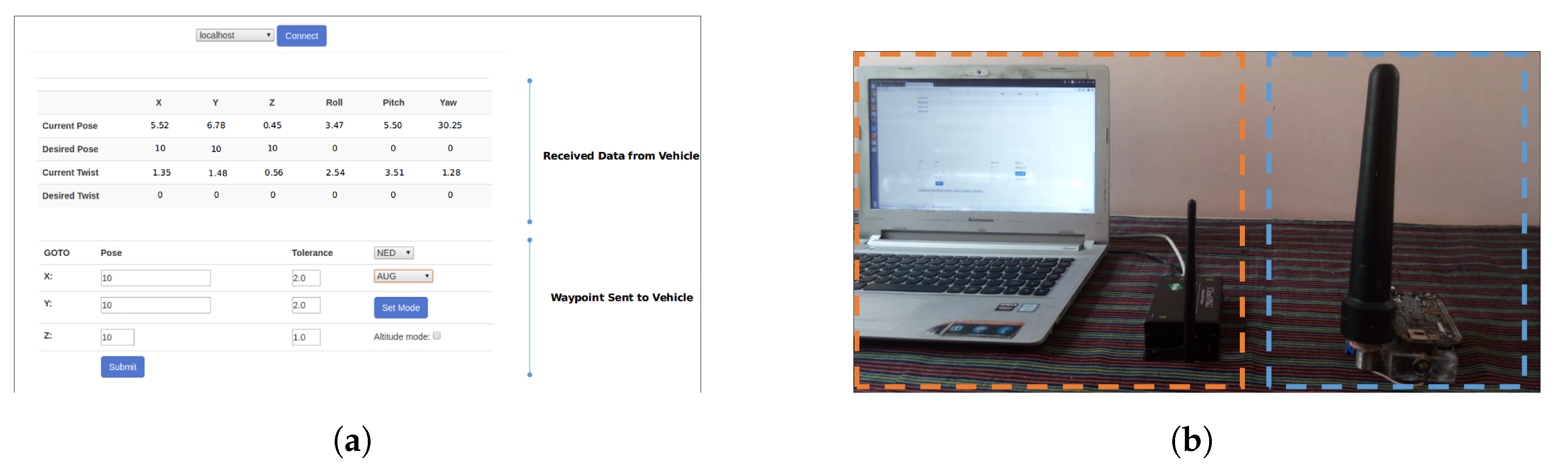
Figure 41.
Communication system experiment. (a) Graphical user interface in the GCS; (b) Communication system experiment.
Figure 41.
Communication system experiment. (a) Graphical user interface in the GCS; (b) Communication system experiment.
Table 1.
HAUG dynamic variables.
Table 1.
HAUG dynamic variables.
| Symbols | Value | Units |
|---|
| Mass (m) | 86.5 | kg |
| Gravitational constant (g) | 9.8 | m/s2 |
| Weight (W) | 847.7 | N |
| Buoyancy force (B) | 847.7 | N |
| Water density () | 1000 | kg/m3 |
| Length (L) | 2.3 | m |
| Diameter (d) | 0.24 | m |
| Centre of gravity (CoG) | | m |
| Centre of buoyancy (CoB) | | m |
| KD0 (from CFD) | 8.8 | - |
| KD (from CFD) | 242 | - |
| KL0 (from CFD) | 0 | - |
| KL (from CFD) | 395 | - |
Table 2.
Weight distribution for the proposed HAUG.
Table 2.
Weight distribution for the proposed HAUG.
| Item | Description | Weight (in kg) |
|---|
| Wings | Composite fibre | 2 |
| Compartment 4 | Composite fibre, aluminium T6 and component weight | 10.7 |
| Compartment 3 | Aluminium T6 and component weight | 11.1 |
| Compartment 2 | Moving mass weight, aluminium T6 and component weight | 18.1 |
| Compartment 1 | Composite Fibre, aluminium T6 and component weight | 22.3 |
| Battery | 24 V lithium battery 110 Ah | 12.3 |
| Weight balancing | Neutral buoyancy weight distribution | 10 |
| | Total weight | 86.5 |
Table 3.
Power specification of each electrical component.
Table 3.
Power specification of each electrical component.
| No. | Component | Voltage | Max. Current |
|---|
| 5 V | 12 V | 24 V |
|---|
| 1 | DVL | | | V | 3.3 A |
| Altimeter | | V | V | 125 mA |
| Bow thruster | | V | | 12.5 A |
| BBB | V | | | 2 A |
| LED strobe | | V | | 1.25 A |
| Motor pump | | | V | 30 A |
| Valve | | | V | 3 A |
| 2 | BBB | V | | | 2 A |
| Arduino | V | | | 280 mA |
| Motor’s moving mass | | V | | 3 A |
| LAN Hub | V | | | 600 mA |
| 3 | UDOO X86 | | V | | 3000 mA |
| Tether fathom | V | V | V | 500 mA |
| LAN Hub | V | | | 600 mA |
| 4 | BBB | V | | | 2 A |
| Rudder | | V | | 1.5 A |
| Elevator | | V | | 1.5 A |
| Poseidon GPS | V | | | 25 mA |
| Spatial Advance IMU | V | | | 100 mA |
| RF | V | | | 1 A |
| Stern thruster | | V | | 17 A |
| Main thruster | | V | | 17 A |
Table 4.
PID value for each controller.
Table 4.
PID value for each controller.
| Parameter | Surge Controller | Yaw Controller | Pitch Controller |
|---|
| Kp | 2 | 0.9 | 0.9 |
| Ki | 0.2 | 0.2 | 0.2 |
| Kd | 0.1 | 7 | 7 |
Table 5.
Micro DVL 600 Performance.
Table 5.
Micro DVL 600 Performance.
| Parameter | Performance | Units |
|---|
| Frequency | 600 | kHz |
| Accuracy | 1 | % ±1 mm/s |
| Maximum altitude | 110 | m |
| Minimum altitude | 0.3 | m |
| Maximum velocity | ±20 | knots |
| Maximum ping rate | 5 | 1/s |
| Maximum transmit | 80 | watts |
| Average power consumption | 2–5 | watts |
| Input voltage | 24 | V ± 2 V |
Table 6.
Spatial Advance Navigation Performance.
Table 6.
Spatial Advance Navigation Performance.
| Parameter | Performance | Units |
|---|
| Roll and pitch | 0.1 | |
| Heading | 0.2 | |
| RTK positioning | 20 | mm |
| MEMS gyroscope | 3 | /h |
| Update rate | 1000 | Hz |
| Shock limit | 2000 | gr |
Table 7.
VA500 Valeport Performance.
Table 7.
VA500 Valeport Performance.
| Parameter | Performance | Units |
|---|
| Acoustic frequency | 500 | kHz |
| Acoustic range | 0.1–100 | m |
| Acoustic resolution | 1 | mm |
| Acoustic beam angle | ±3 | |
| Pressure range | 300 | bar |
| Pressure accuracy | ±0.01 | % Full-scale |
| Pressure resolution | 0.001 | % Full-scale |
| Type of pressure sensor | Temperature-compensated piezoresistive | |
Table 8.
Poseidon GPS antenna performance.
Table 8.
Poseidon GPS antenna performance.
| Parameter | Performance | Units |
|---|
| Maximum pressure rating | 300 | bar |
| Noise | 2 | dB |
| Antenna element gain | 4 | dBiC |
| Input voltage | 2.5 to 16 | V DC |
Table 9.
Sensor noise.
| Parameter | Value | Units |
|---|
| Accelerometer noise in 3 axes | , | |
| , |
| , |
| Accelerometer bias noise in 3 axes | ,
,
| |
| Gyro noise in 3 axes | ,
,
| |
| Gyro bias noise | 0, 0, 0 | |
| DVL noise in 3 axes | ,
| |
| GPS noise | | |
| Depth sensor noise | | |


 ,
, 


