Figure 1.
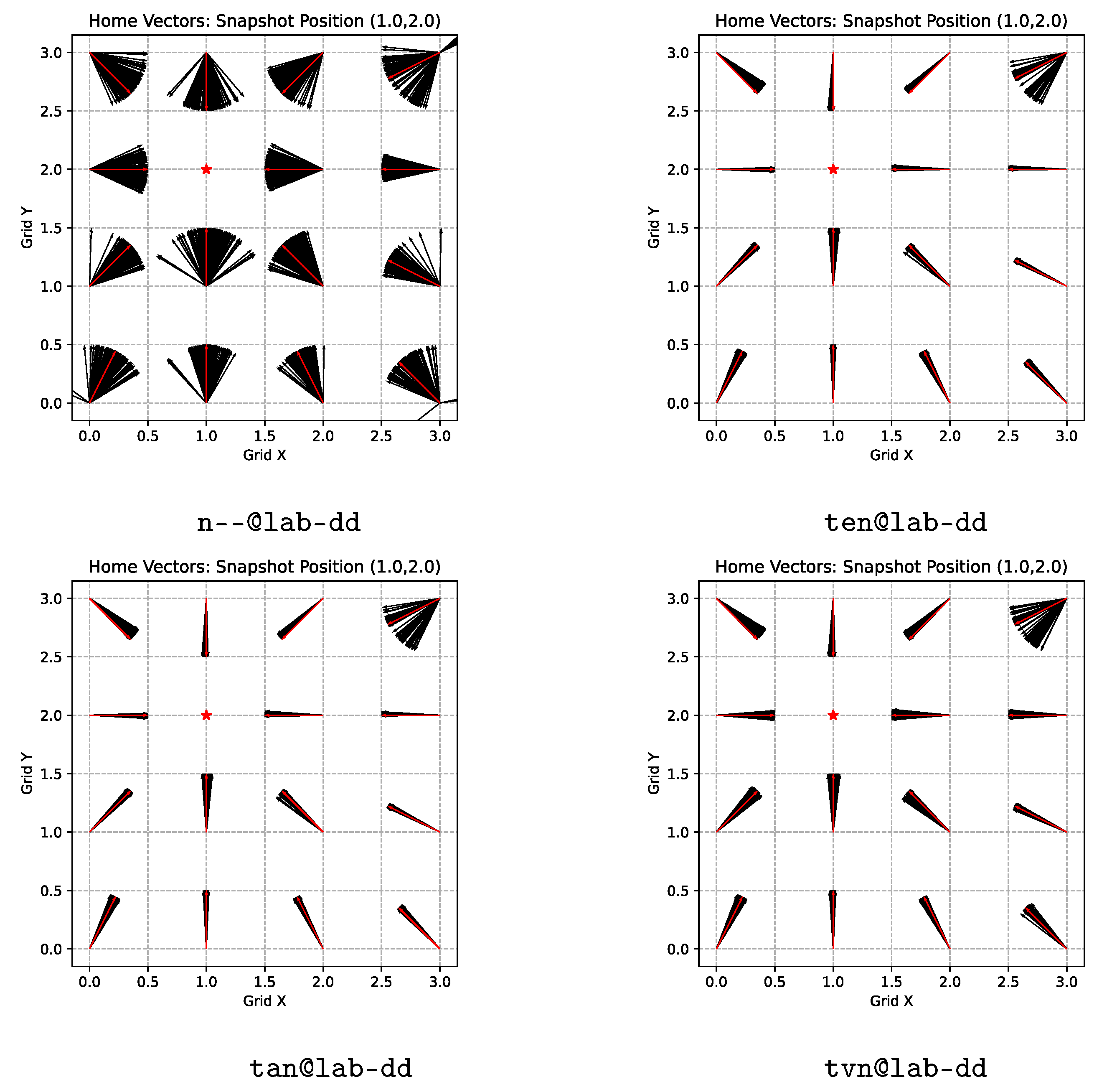
Overview and exemplary results of the proposed tilt-correction warping methods; see the text for a detailed explanation of the algorithm. The vector-field plots below visualize the home-direction estimates by warping at each position over the different tilts in the database, in case of the original warping algorithm without tilt correction (left) and of the proposed extension incorporating a search for the tilt correction of the current view image. Warping with tilt-corrected images (right) shows a markedly reduced spread of the direction estimates. The sample without tilt correction is produced from the n--@lab-dd experiment. The sample with tilt correction is produced from the pen@lab-dd experiment, showing the results of one of the heuristic search strategies, pattern search.
Figure 1.
Overview and exemplary results of the proposed tilt-correction warping methods; see the text for a detailed explanation of the algorithm. The vector-field plots below visualize the home-direction estimates by warping at each position over the different tilts in the database, in case of the original warping algorithm without tilt correction (left) and of the proposed extension incorporating a search for the tilt correction of the current view image. Warping with tilt-corrected images (right) shows a markedly reduced spread of the direction estimates. The sample without tilt correction is produced from the n--@lab-dd experiment. The sample with tilt correction is produced from the pen@lab-dd experiment, showing the results of one of the heuristic search strategies, pattern search.
Figure 2.
Progressive violations of the planar-motion assumption. The panoramic camera is visualized by the outermost lens as it appears in an ultrawide-angle fisheye lens system. (
a) depicts the planar-motion assumption underlying the original warping method. None of the cameras is tilted and the horizontal plane (red, dashed line) of each intersects with the optical center (black dots) of the other, i.e., both horizontal planes are identical. (
b) depicts a first violation of this planar-motion assumption by tilting one of the cameras out of this shared horizontal plane. The optical center of this tilted camera still lies within the horizontal plane of the not-tilted camera, but not vice versa. This intermediate case is the one handled by our newly proposed method, when tilt correction is applied to the view of the camera depicted on the right side. Finally, (
c) depicts the more general case of both cameras tilted out of a shared plane connecting the optical centers. The horizontal planes now intersect outside of both of the cameras. This more general case is left for future work and might also extend to or even require out-of-plane translations (see [
11] for the case of the generalized 3D-warping).

Figure 3.
Depiction of a coordinate system tilted according to the two proposed representations. The axis-angle representation (a) describes the tilt as a single rotation by a small angle about the tilt axis , which lies within the reference plane of the nontilted coordinate system and is described relative to the X-axis by an angle . This angle does not correspond to a real rotation of the robot as it just specifies the axis of rotation. Furthermore, the angle typically is not small, i.e., it can range from 0 to 360 as the robot may tilt in any direction. The roll-pitch representation (b) describes the tilt as two consecutive small rotations and about the X- and Y-axis which span the reference plane of the nontilted coordinate system. As two rotations generally do not commute, the order of these two matters: the X-axis rotation by is always carried out first, i.e., the Y-axis rotation is about the already tilted axis . The green, dotted coordinate system with the axis indicates this intermediate step where only the X-axis rotation is performed. In both representations, the total amount of tilt is given by the angle between the nontilted and tilted Z-axis, which is pointing upwards: .

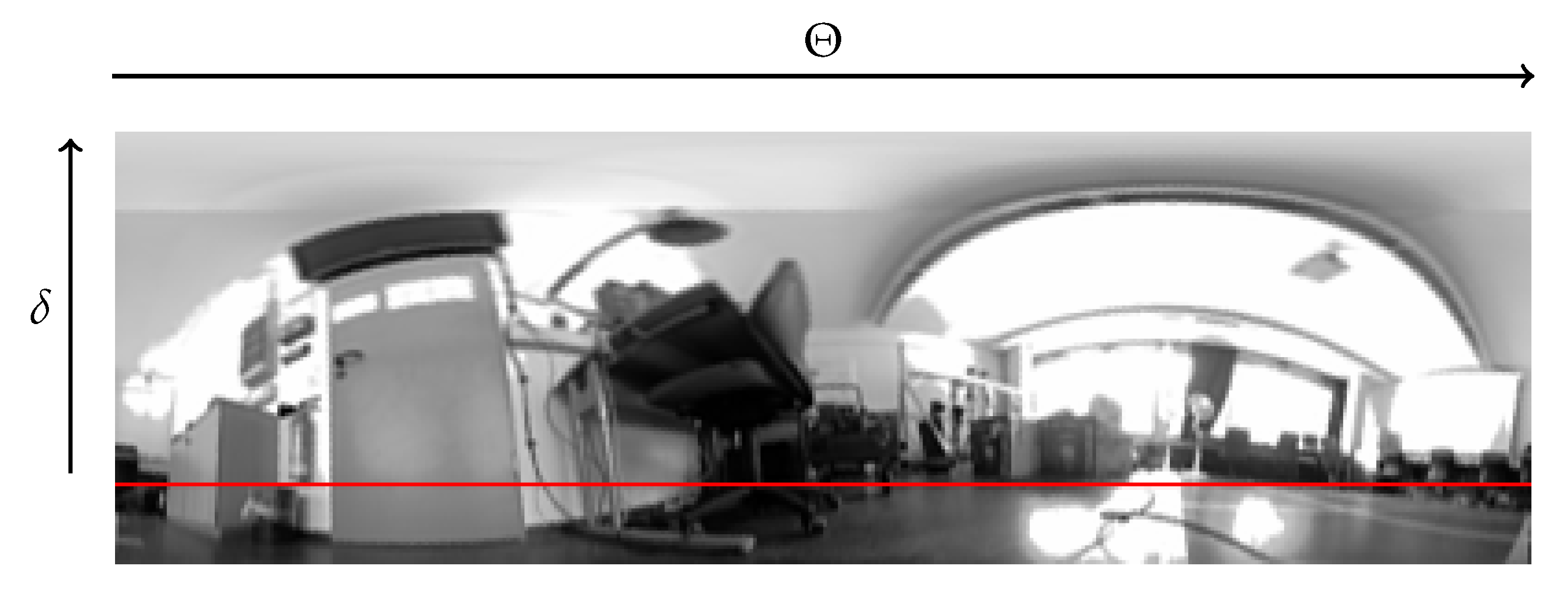
Figure 4.
Angular coordinates of pixels in the panoramic image: modified spherical coordinates where the vertical angle is measured from the horizon (red line) which lies somewhere inside the vertical range of the image. The horizontal angle runs from left to right in the reading direction.
Figure 4.
Angular coordinates of pixels in the panoramic image: modified spherical coordinates where the vertical angle is measured from the horizon (red line) which lies somewhere inside the vertical range of the image. The horizontal angle runs from left to right in the reading direction.
Figure 5.
Example of a tilt-corrected panoramic image showing white invalid regions introduced at the bottom to prevent out of bounds accesses. This sample image is produced using the exact tilt-correction solution with a nearest-neighbor interpolation.
Figure 5.
Example of a tilt-corrected panoramic image showing white invalid regions introduced at the bottom to prevent out of bounds accesses. This sample image is produced using the exact tilt-correction solution with a nearest-neighbor interpolation.
Figure 6.
Exhaustive search: depiction of the uniform search grid (red dots) of spacing . The dots mark the tilt configurations which are systematically probed to find the one minimizing the warping objective. The depicted grid has a total of 225 points, i.e., 15 tilt configurations per axis. The black lines mark the center axes of the search space, crossing at the tilt configuration.
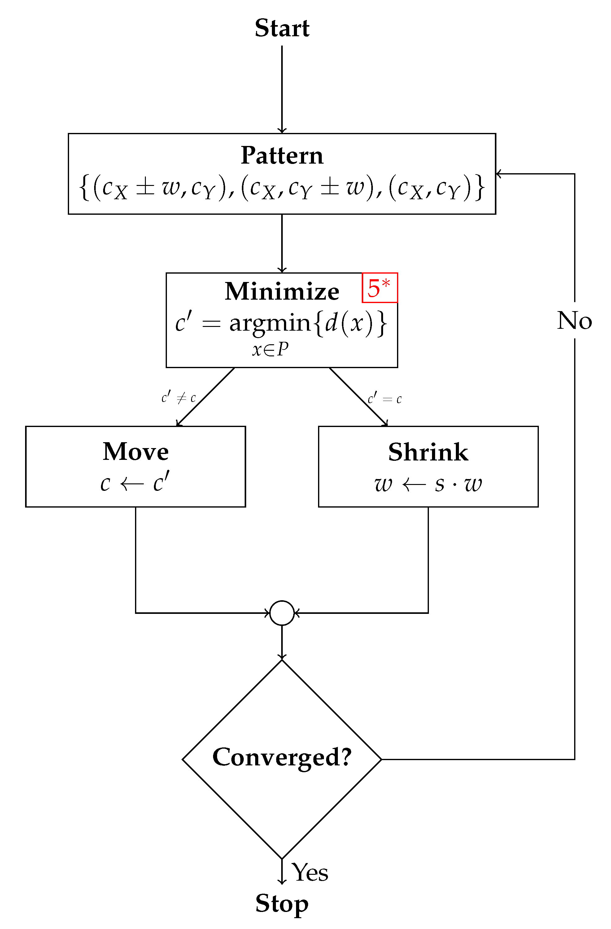
Figure 7.
Flowchart of the pattern search algorithm. A red number at the corner of a box indicates the number of evaluations of the warping objective necessary at that step. However, by remembering already evaluated points (not all change at each update step), this number can in practice be reduced to 3 or 4 evaluations per iteration (to indicate this, the number is marked by a red star). Arrows annotated with inequalities indicate mutually exclusive branches and should be read like decision boxes, which are not drawn to keep the figure more compact.
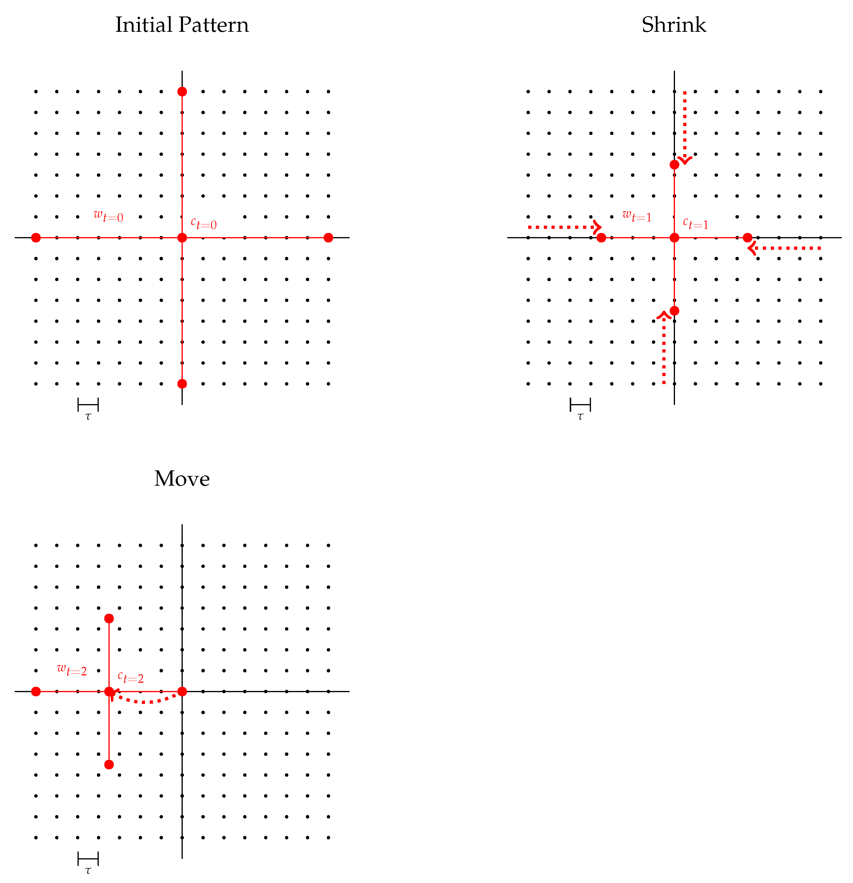
Figure 8.
Pattern search: depiction of a sequence of the shrink and move operation starting from an initial pattern covering the whole search space (black dots). The spacing between the dots indicates the threshold resolution of the search pattern to test for convergence. The black lines mark the center axes of the search space, crossing at the tilt configuration.
Figure 9.
Flowchart of the Nelder–Mead search algorithm. A red number at the corner of a box indicates the number of evaluations of the warping objective necessary at that step. Right before merging all paths, red numbers indicate the total number of evaluations along each path. Arrows annotated with inequalities indicate mutually exclusive branches and should be read like decision boxes, which are not drawn to keep the figure more compact.
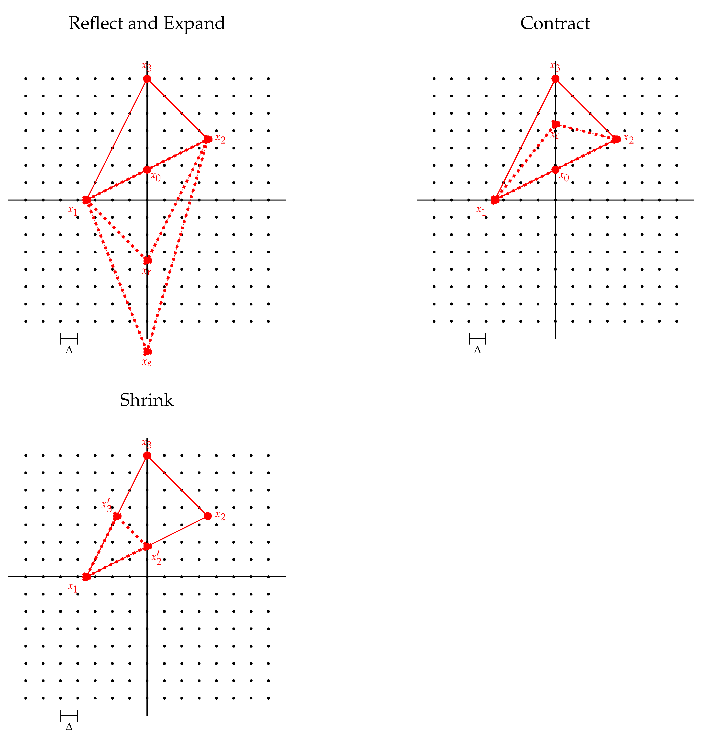
Figure 10.
Nelder–Mead (simplex) search: depiction of the four update operations on the search simplex superimposed on the uniform search grid (black dots). Starting from the ordered set of vertices , an improvement is sought by reflecting , expanding , or contracting along the line connecting the worst candidate to the centroid between the best candidates. If no such improvement is found, the simplex shrinks towards the best candidate . The black lines mark the center axes of the search space, crossing at the tilt configuration.
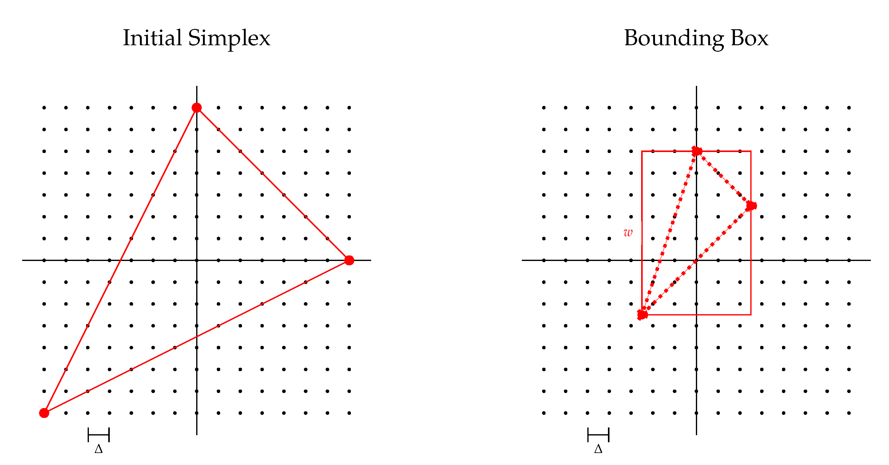
Figure 11.
Nelder–Mead (simplex) search. The left figure shows the initialization of the simplex covering most parts of the search space by placing the vertices at two edges and a corner of the search space. The right figure shows the axis-aligned bounding box used to estimate the size of the simplex by the length w of the longer side of the box.
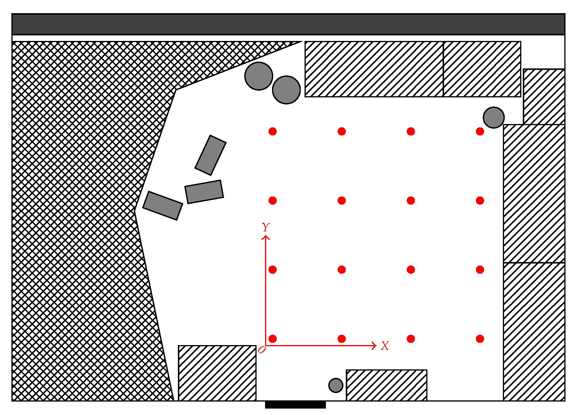
Figure 12.
Layout of the laboratory room where the LAB database was collected. The database covered an area of in steps of . The grid of image locations is marked in red. The whole room had a size of . The areas comprising furniture such as cupboards, desks, or chairs are marked by hatched regions, and gray boxes and circles mark the position and rough shape of small items such as card boxes and fans. The door of the room is marked by the black bar at the bottom wall. The cross-hatched area on the left half of the room comprised a variety of laboratory equipment, including robots, cables, and tools. The dark gray area along the top wall of the room marks the window facade, which was partially covered by curtains.
Figure 13.
Layout of the living room where the LIV database was collected. The database covers an area of in steps of . The grid of image locations is marked in red. The whole room had a size of and each of the furniture items was at least partially visible at one of the locations. The areas comprising furniture such as cupboards, tables, chairs, or sofas are marked by hatched regions, and gray boxes and circles mark the position and rough shape of decor items. The three doors of the room are marked by the black bars. The dark gray area along the right wall of the room marks the window facade, which was partially covered by shutters and curtains.
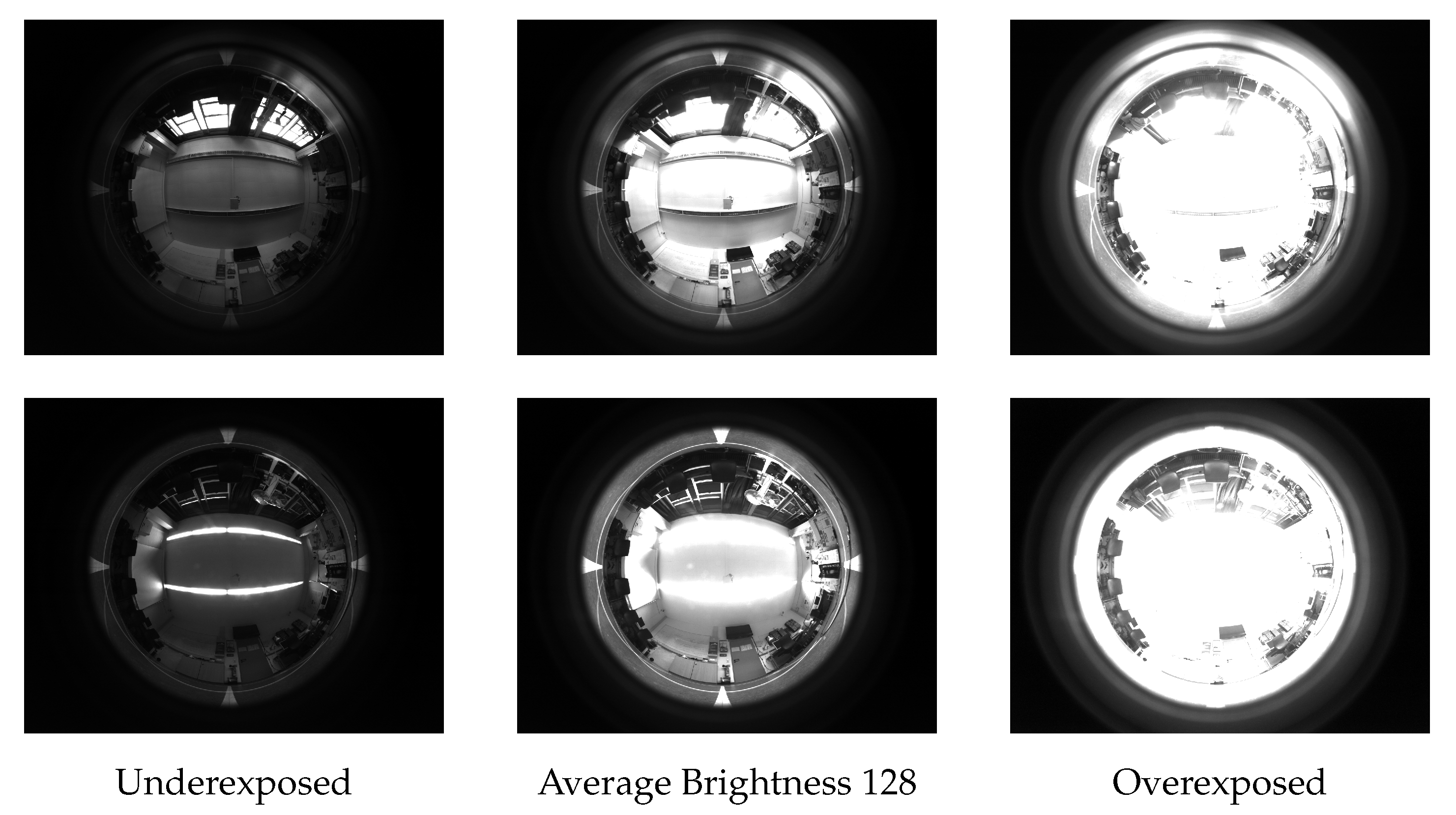
Figure 14.
Sample images from the LAB database. All images were collected at position of the database grid in the , i.e., no-tilt, configuration. The images of the top row were collected during the day with bright light shining through the windows and artificial lighting turned off. The images of the bottom row were collected during the night at the same pose. At night there was no light shining through the windows and the artificial lighting was turned on. There were no changes to the environment between the two variants besides the illumination conditions.
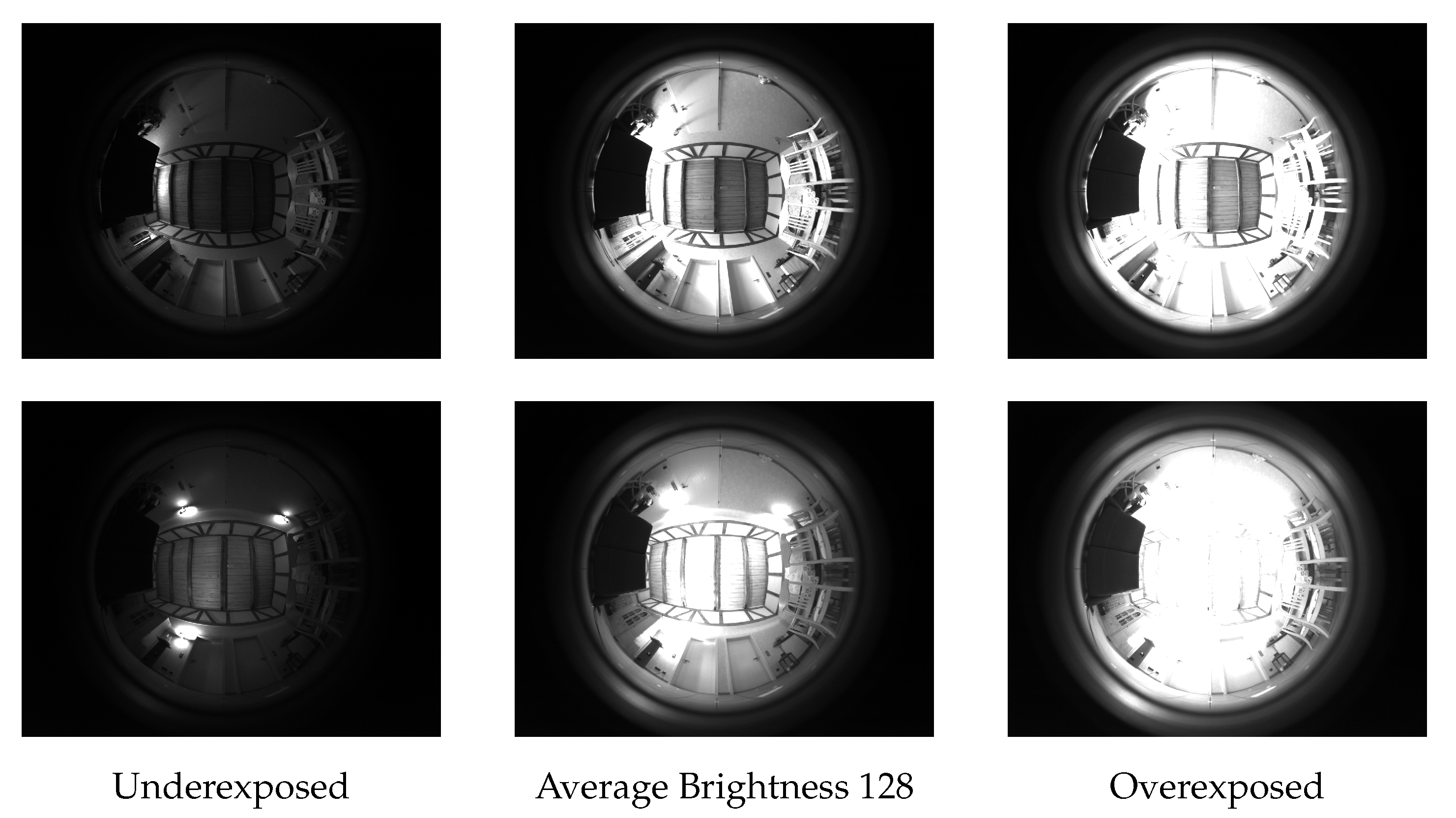
Figure 15.
Sample images from the LIV database. All images were collected at position of the database grid in the , i.e., no-tilt, configuration. The images of the top row were collected during the day with bright light shining through the windows and artificial lighting turned off. The images of the bottom row were collected during the night at the same pose. At night there was no light shining through the windows and the artificial lighting was turned on. There were no changes to the environment between the two variants besides the illumination conditions.
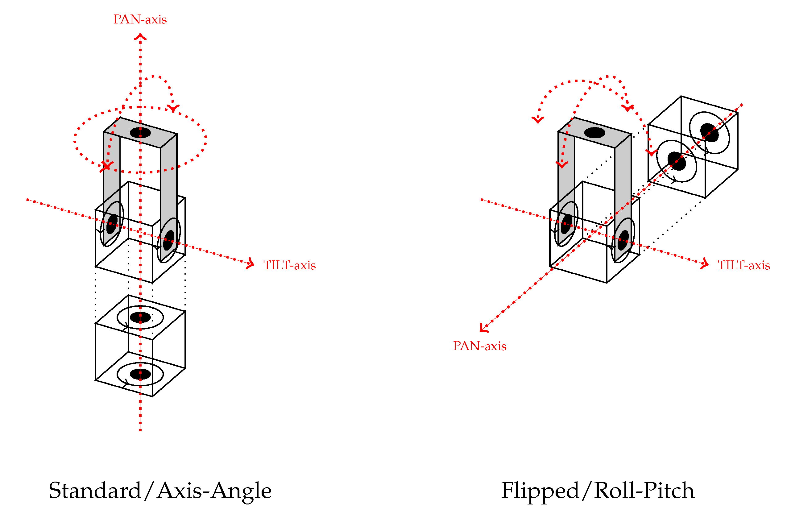
Figure 16.
Two configurations of the pan–tilt unit (PTU). The standard configuration (
left) is the one giving the PTU its name with the two servo modules mounted on top of each other. This configuration matched the axis-angle representation of tilt where the PAN-axis rotation selected the tilt axis and the TILT-axis rotation the amount of tilt. However, with the camera mounted rigidly on top of the setup, this caused a change of view direction due to the panning as well and thus coupled the view direction to the tilt. To get a configuration which decoupled the view direction from the tilt, the PTU was flipped on its side (
right) by mounting it at a 90° angle about the TILT-axis while keeping the camera mount upright. This way, the PAN- and TILT-axis spanned the horizontal plane and could be associated with the X- and Y-axis of the roll-pitch representation. See
Figure 3 for a depiction of the two tilt representations.
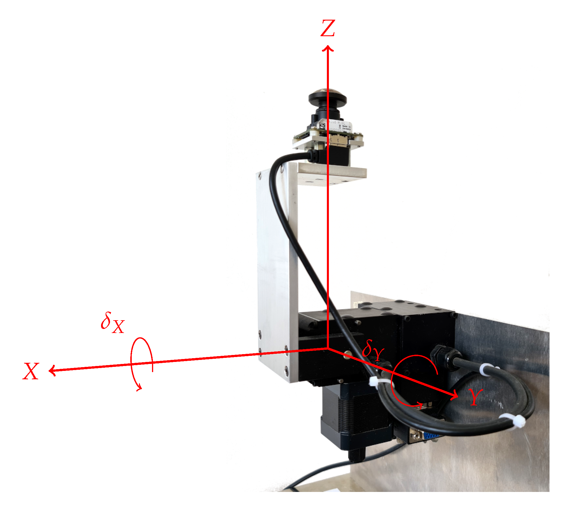
Figure 17.
PTU in flipped/roll-pitch configuration. Photo of the modified PTU and camera mount for decoupling the view direction from the tilt. See
Figure 16 for a schematic view of this configuration. The coordinate system associating the X- and Y-axis of the roll-pitch representation with the PAN- and TILT-axis, respectively, is drawn in red. The origin is placed at the intersection of the PAN- and TILT-axis. The camera mount is centered above (along the Z-axis) the origin.
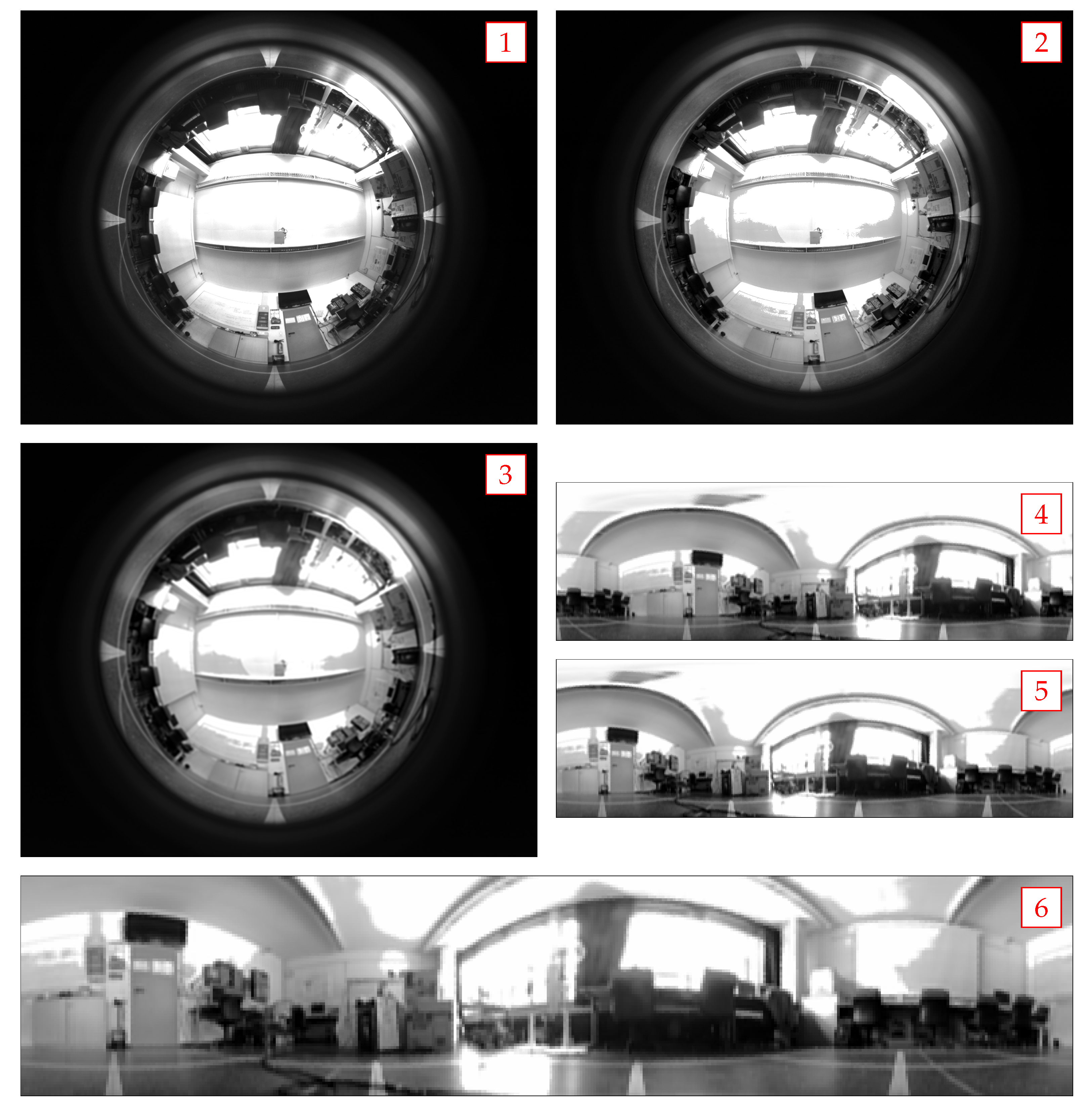
Figure 18.
Path of a sample image from the day variant of the LAB database at position without tilt through the image processing pipeline: (1) original image from the database; (2) improved contrast after histogram equalization; (3) low-pass-filtered using a 3rd-order Butterworth filter with relative cutoff frequency of 0.2; (4) unrolled panoramic representation; (5) simulated rotation of by horizontal left shift with wrap-around; (6) cropping of upper to remove the distorted ceiling and potentially invalid regions at the top.
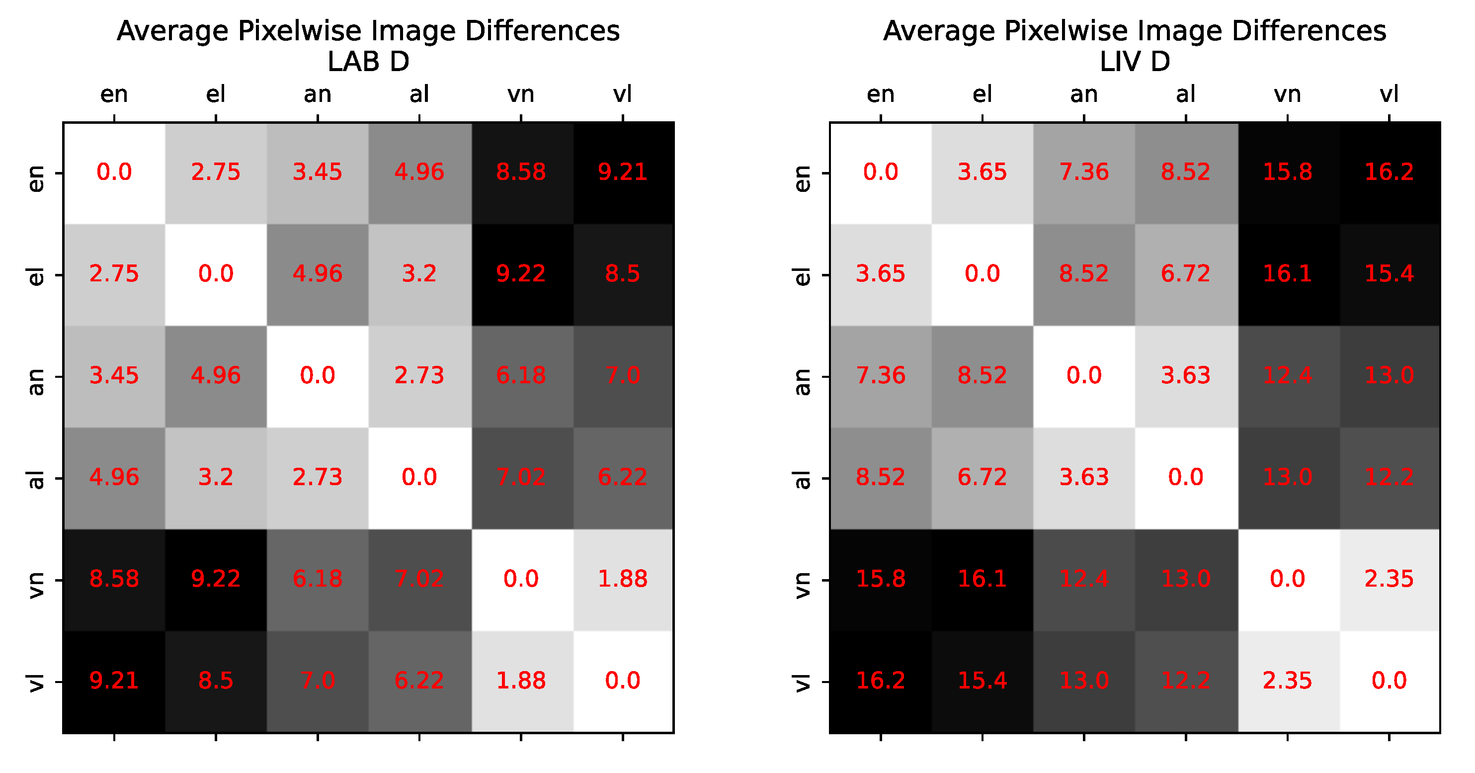
Figure 20.
Plot of the average pixelwise image differences between all tilt-correction solutions. The LAB and LIV database are reported separately as the ranges of tilt and thus the expected deviations were different (LIV comprised more tilt). The results were averaged by taking the mean per method over all images contained in the database. For the tilt correction, the ground-truth tilt parameters as recorded in the database were used. The image difference measure is a symmetric distance measure, therefore the plotted matrices are symmetric about the main diagonal as well. With a stronger approximation, the effect of the different interpolation methods becomes smaller. The exact e* and approximate solutions a* are more similar to each other than to the vertical approximation v*.
Figure 21.
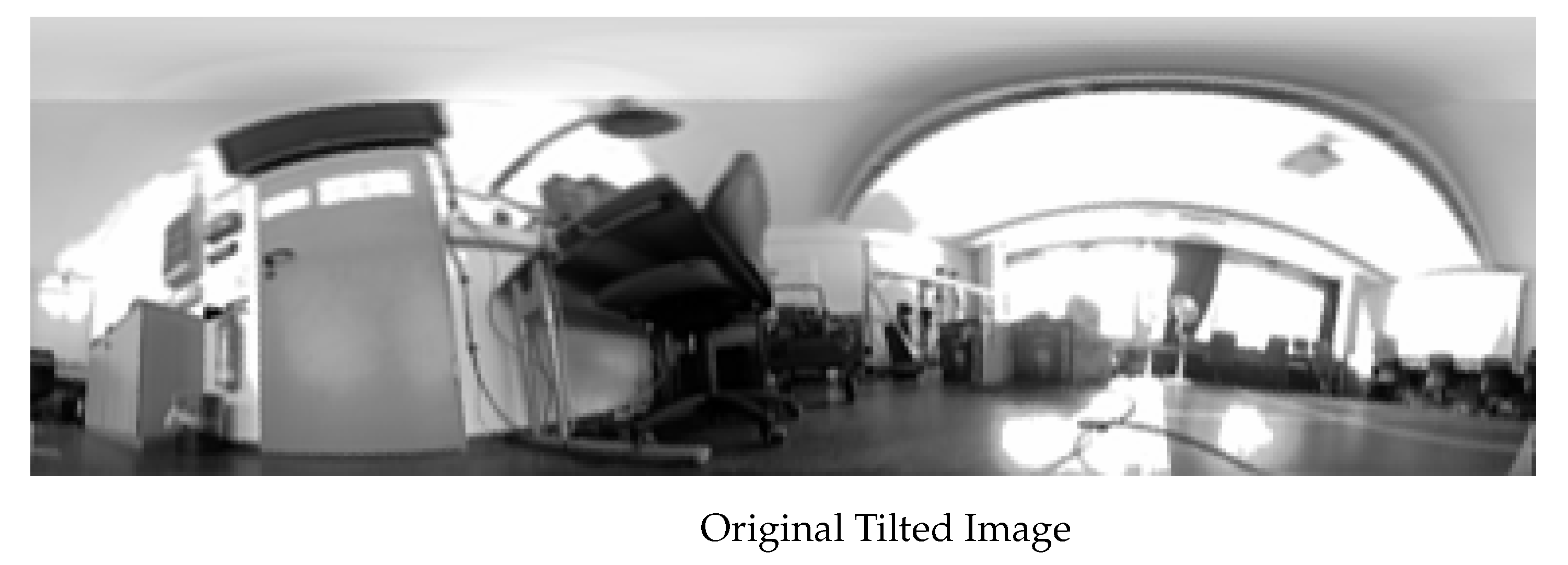
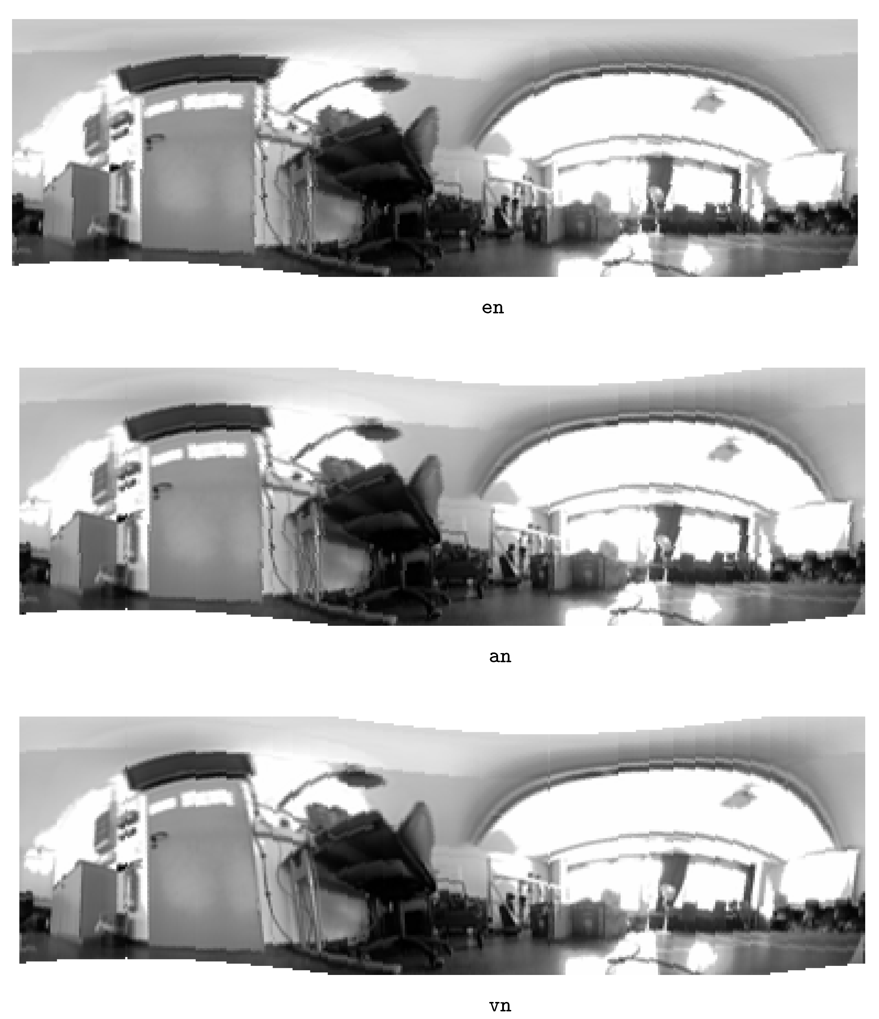
Sample image from the LAB database at position in the most extreme tilt configuration. The original tilted image is shown at the top. Below is the image after tilt correction based on the ground truth using the three approximation levels with a nearest-neighbor interpolation. Invalid regions appear at the bottom of the exact solution and at the top and bottom of the approximate solutions. The jagged edges are an artifact of the nearest-neighbor interpolation. While the exact and approximate solutions clearly straighten out most of the edges, the vertical approximation still seems to be more similar to the original, tilted image than to the other tilt-corrected images, in particular in regions farther away from the horizon. The effects become most obvious when looking at the door, which should be perfectly straight and upright after tilt correction. Note that this image difference experiment omits the last two preprocessing steps of rotating and cropping the image, and thus invalid regions can be seen at the top of the approximate and vertical solution.
Figure 21.
Sample image from the LAB database at position in the most extreme tilt configuration. The original tilted image is shown at the top. Below is the image after tilt correction based on the ground truth using the three approximation levels with a nearest-neighbor interpolation. Invalid regions appear at the bottom of the exact solution and at the top and bottom of the approximate solutions. The jagged edges are an artifact of the nearest-neighbor interpolation. While the exact and approximate solutions clearly straighten out most of the edges, the vertical approximation still seems to be more similar to the original, tilted image than to the other tilt-corrected images, in particular in regions farther away from the horizon. The effects become most obvious when looking at the door, which should be perfectly straight and upright after tilt correction. Note that this image difference experiment omits the last two preprocessing steps of rotating and cropping the image, and thus invalid regions can be seen at the top of the approximate and vertical solution.


Figure 22.
Home vector field plots comparing the tilt-correction solutions with a nearest-neighbor interpolation on the true tilt strategy. One sample snapshot location from the LAB DxD dataset is shown. The red arrows show the true home direction per position, the black arrows show the estimates obtained by the applied method—as there were 121 images per position in the dataset, there are also 121 home-direction estimates per position even though they might overlap in these plots. For this test, the snapshot position near the middle of the grid was chosen and hence the arrows should ideally point there. The location in the top right corner is a known “bad spot” of the LAB environment, near to multiple furniture items.
Figure 23.
Home vector field plots comparing the tilt search strategies with a nearest-neighbor interpolation on the exact tilt-correction solution; the same sample snapshot location from the LAB DxD dataset as in
Figure 22 is shown.
Figure 23.
Home vector field plots comparing the tilt search strategies with a nearest-neighbor interpolation on the exact tilt-correction solution; the same sample snapshot location from the LAB DxD dataset as in
Figure 22 is shown.
Figure 24.
Home vector field plots comparing the tilt search strategies with a nearest-neighbor interpolation on the exact tilt-correction solution; one sample snapshot location from the LIV DxD dataset is shown. As the LIV database had 225 tilt configurations (images) per position, there are 225 potentially overlapping black arrows per position showing the estimated home directions. For this test, the snapshot position near the middle of the grid was chosen and hence the arrows should ideally point there.
Figure 25.
Distribution of the home direction error and tilt correction error , exemplarily shown for the exhaustive tilt search using an exact tilt correction with a nearest-neighbor interpolation on the LAB DxD dataset (een@lab-dd). The median yields the better measure to summarize the homing performance, compared to the mean, as the error of the home direction tends to show a skewed distribution with a long tail of rarely occurring large errors. Though not as pronounced, the tilt correction error behaves similarly.
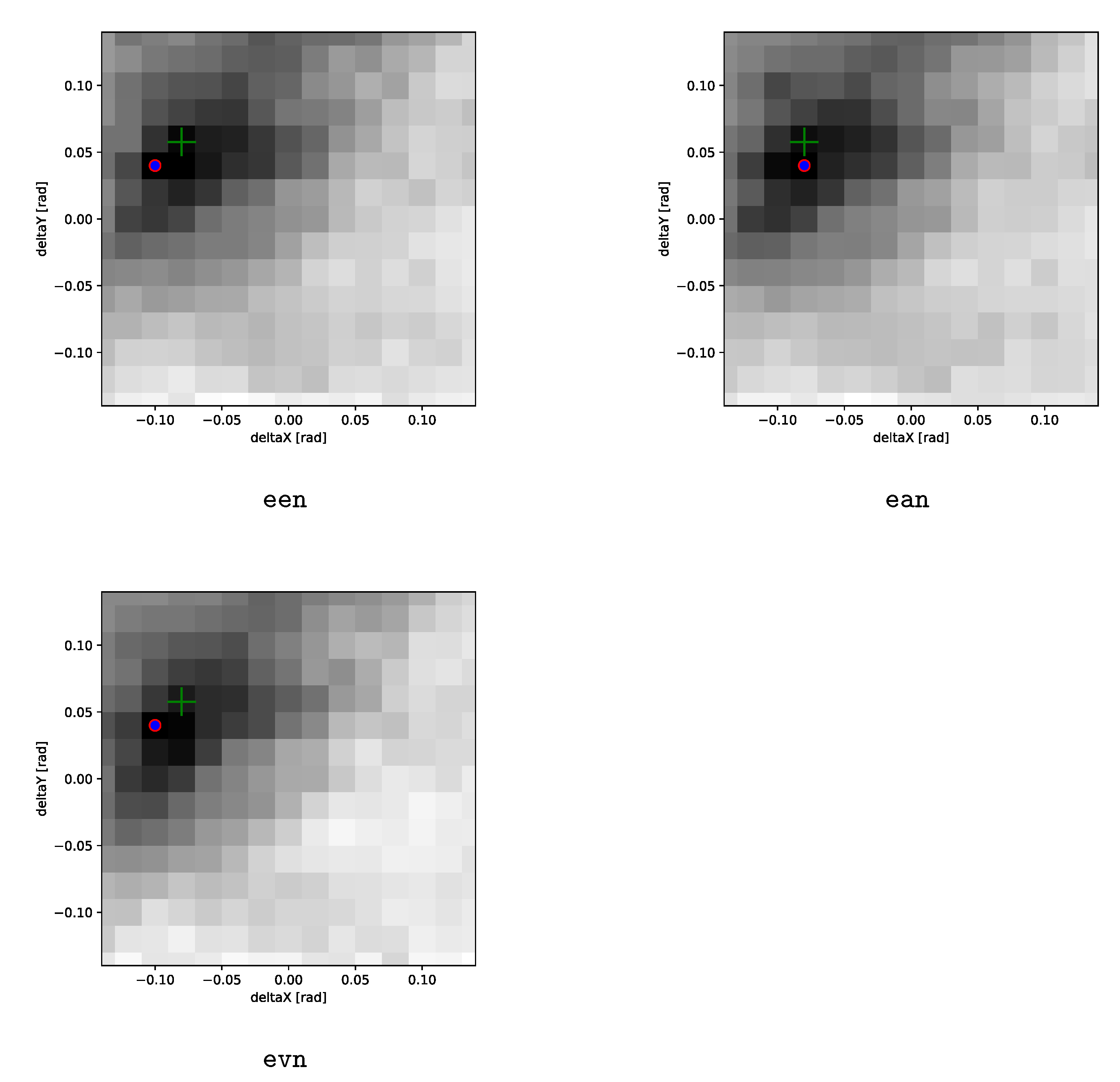
Figure 26.
Visualization of the exhaustive search with the different approximations of the tilt correction and with a nearest-neighbor interpolation. For each of the tilt configurations from the exhaustive search parameter grid, the
d value of the corresponding warping run, i.e., the objective function value, is plotted. The darker the pixel, the lower the
d, and hence the better the match of the tilt correction. The green cross marks the location of the ground-truth tilt parameters, i.e., the expected minimum, and the red-blue circle marks the minimum found by the search procedure. For all tilt-correction solutions, good matches are clearly concentrated around the true minimum with the objective function values decreasing towards it. A pronounced valley is visible and the overall terrain is not “too bumpy”, as necessary for the heuristic search methods to be applicable. The two approximations show a slightly more elongated valley of potential or near matches. In these cases, the estimated minimum of all solutions is between 1
and 2
off of the true tilt configuration, i.e., at one of the adjacent grid points. This particular sample was produced from the LAB DxD dataset taking the snapshot image at position
with no tilt and with an added rotation of
and the current view image at position
in the
tilt configuration with an added rotation of
. The rotation added to the current view image caused the tilt configuration to be rotated as well to the
location marked by the green cross (see Equation (
31) for more details).

Figure 27.
Visualization of the pattern search strategy pen. As a reference, the exhaustive search heatmap of the een strategy (see
Figure 26 for information on the selected image pair) is plotted as the background. The green cross marks the location of the ground truth tilt parameters, i.e., the expected minimum. At each step, the state of the search pattern is visualized as a red cross connecting the test points. At the final step, the red-blue filled center circle marks the minimum found by the search procedure. After only four update steps the pattern is already centered at the top left quadrant containing the minimum. In total, only seven update steps corresponding to 22 warping evaluations are necessary to find a good approximation of the tilt correction—this is in contrast with the 225 evaluations of the exhaustive search grid. According to Table 11, this actually represents a worse-than-average performance with a mean and median number of evaluations of about 18 if tilt is present.
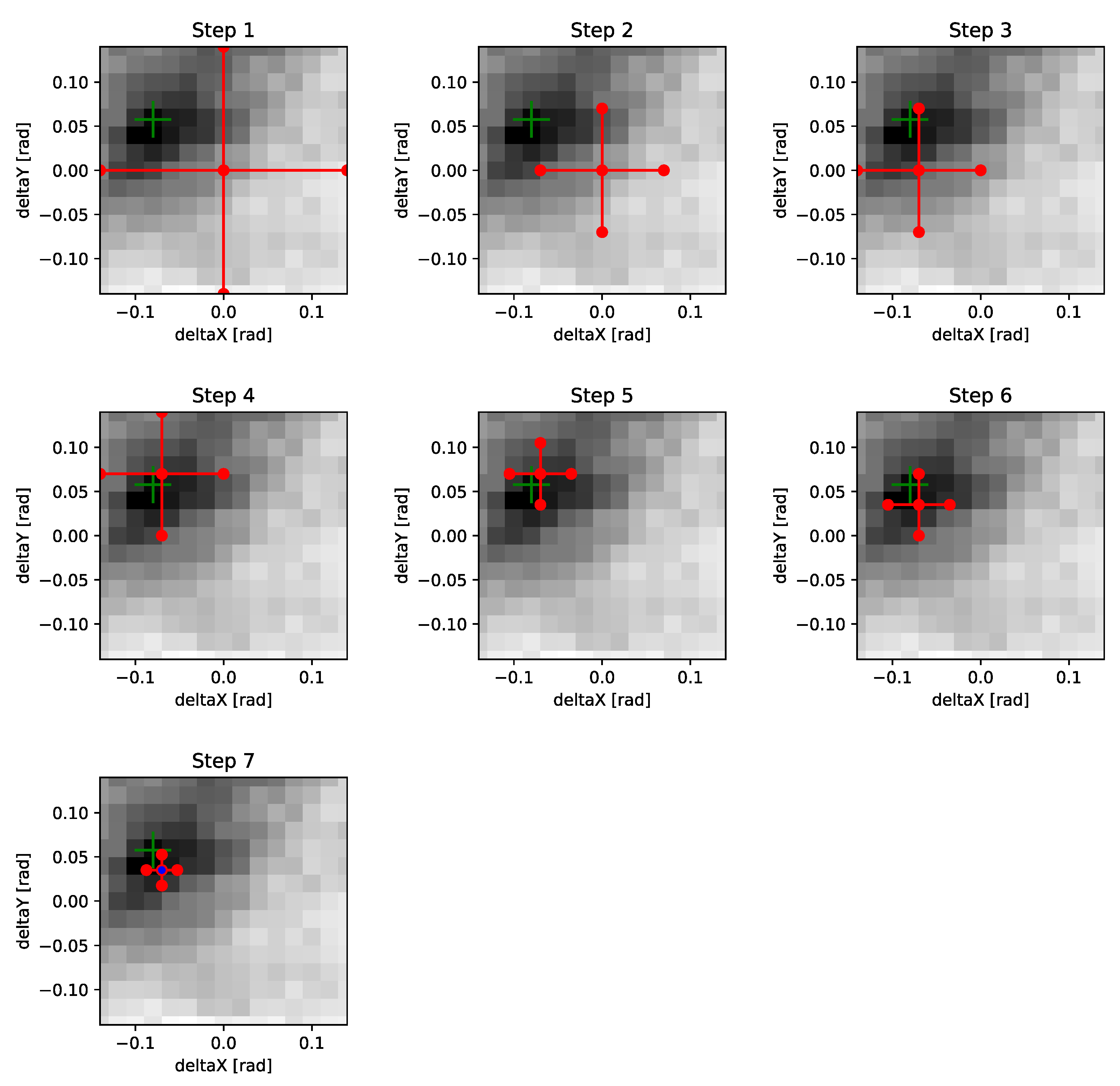

Figure 28.
Visualization of the Nelder–Mead search strategy sen. As a reference, the exhaustive search heatmap of the een strategy (see
Figure 26 for information on the selected image pair) is plotted as the background. The green cross marks the location of the ground truth tilt parameters, i.e., the expected minimum. At each step, the state of the search simplex is visualized as a red triangle connecting the test points. At the final step, the red-blue filled circle marks the minimum found by the search procedure. After only three update steps, the minimum already lies inside the simplex. In total, only eight update steps corresponding to 13 warping evaluations are necessary to find a good approximation of the tilt correction—this is in contrast with the 225 evaluations of the exhaustive search grid. Note that most of the update steps were contractions, requiring two evaluations of the warping objective. However, in steps 2, 4, and 6 the reflected point, which was computed before the contraction, would be outside of the search range causing the warping evaluation to be skipped, reducing the number of evaluations to one. According to Table 11, this actually represents a slightly better-than-average performance with respect to the median number of evaluations of 15 (and a mean number of 30), if tilt is present.

Figure 29.
Runtime vs. home-direction error of all tilt-correction search method variants pooled over all datasets per LAB/LIV database. Both metrics are summarized using the median, which in case of the home direction is definitely the better measure as discussed in
Figure 25. For the runtime, the simplex strategies show a difference between median and mean. According to the latter, the simplex strategies would be placed slightly behind the pattern search in terms of runtime. However, the median was chosen for the runtime as well, to treat both metrics consistently. In terms of runtime, there is not much difference between the two databases, and the difference in home-direction errors probably stems from the increased range of tilt and the more difficult environment of the LIV database. The methods form two broad clusters: the fast but more error-prone heuristic search strategies clustering around 400
and the slow but precise exhaustive search between 5
to 6
. The effects of the choice of the tilt-correction method are subordinate and the interpolation is behaving rather inconsistently between the two databases.

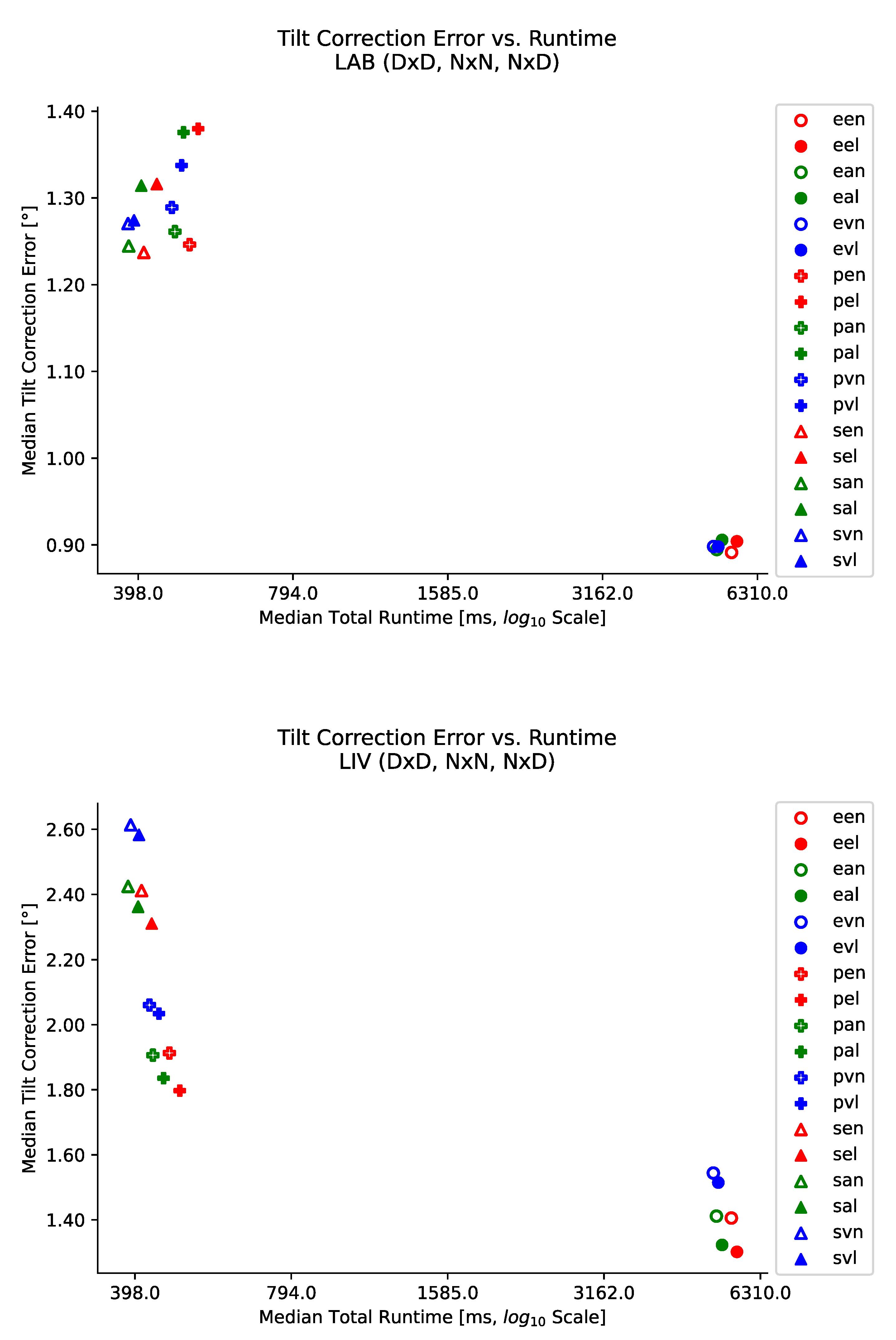
Figure 30.
Runtime vs. tilt-correction error of all tilt-correction search method variants pooled per database. Similar to
Figure 29, both metrics are summarized using the median instead of the mean. Again, the different error ranges between the databases probably stem from the increased range of tilt and the more difficult environment of the LIV database. Similar to the homing performance, the methods form the two clusters of heuristic and exhaustive search strategies with the tilt-correction methods being the secondary effect and the effect of the interpolation switching between the two databases.
Table 1.
Identifiers of the six tilt-correction methods. The identifiers are composed of the initial letters of the methods, naming the tilt correction solution first, followed by the interpolation scheme.
Table 1.
Identifiers of the six tilt-correction methods. The identifiers are composed of the initial letters of the methods, naming the tilt correction solution first, followed by the interpolation scheme.
| | Nearest Neighbor | Bilinear |
|---|
| Exact |
en
|
el
|
| Approximate |
an
|
al
|
| Vertical |
vn
|
vl
|
Table 2.
Identifiers of the tilt-correction warping schemes. The identifier of the tilt (search) strategy is prepended to that of the tilt-correction method (see
Table 1). The Nelder–Mead search uses s for the simplex method. The
true tilt strategy applied a single ground-truth tilt correction as recorded in the databases, before running warping once. The
none tilt strategy was a baseline test running warping without any tilt correction. This baseline was the same for both interpolation schemes as there was nothing to interpolate. In total, there were 25 combinations.
| Nearest-Neighbor Interpolation |
|---|
| | Exact | Approximate | Vertical | None |
| True |
ten
|
tan
|
tvn
|
-
|
| Exhaustive |
een
|
ean
|
evn
|
-
|
| Pattern |
pen
|
pan
|
pvn
|
-
|
| Nelder–Mead |
sen
|
san
|
svn
|
-
|
| None |
-
|
-
|
-
|
n--
|
| Bilinear Interpolation |
| | Exact | Approximate | Vertical | None |
| True |
tel
|
tal
|
tvl
|
-
|
| Exhaustive |
eel
|
eal
|
evl
|
-
|
| Pattern |
pel
|
pal
|
pvl
|
-
|
| Nelder–Mead |
sel
|
sal
|
svl
|
-
|
| None |
-
|
-
|
-
|
n--
|
Table 3.
Configuration of the image distance and scale-plane stack computation. A scale-plane stack of 9 distance images was computed with a scale factor up to 2.0 using a modified NSAD column distance measure, adapted to handle the invalid regions due to the tilt-correcting image transformations.
Table 3.
Configuration of the image distance and scale-plane stack computation. A scale-plane stack of 9 distance images was computed with a scale factor up to 2.0 using a modified NSAD column distance measure, adapted to handle the invalid regions due to the tilt-correcting image transformations.
| Distance Measure | Num. Scale Planes | Max. Scale Factor |
|---|
| NSAD with invalid region handling | 9 | 2.0 |
Table 4.
Number of steps, search range, and resolution of the warp parameter search space used by MinWarping.
Table 4.
Number of steps, search range, and resolution of the warp parameter search space used by MinWarping.
| Search Steps | Search Range | Resolution |
|---|
| | |
| | |
Table 5.
Configuration of the MinWarping searcher. MinWarping was configured to perform a double search, i.e., a second run with exchanged snapshot/current view, with compass acceleration.
Table 5.
Configuration of the MinWarping searcher. MinWarping was configured to perform a double search, i.e., a second run with exchanged snapshot/current view, with compass acceleration.
| Searcher | Compass Acceleration | Partial- | Double- | Fine-Search |
|---|
| MinWarping | Yes, Sum | No | Yes | No |
Table 6.
Range and resolution parameters used by the tilt search strategies. All three strategies were set up to cover the same symmetric search range of up to of tilt per axis in the roll-pitch representation. This range comprised the maximum tilt of both databases (i.e., the range of the LIV database) and was used for experiments on both. The grid and pattern search resolution also matched the step size between tilt configurations of the LIV database, and the simplex threshold was derived from these as , as described earlier.
| Search Range | Grid | Pattern | Simplex |
|---|
| | | |
Table 7.
Median of the home-direction error in degrees. The methods are grouped by tilt (search) strategy first and then arranged by tilt correction and interpolation method. In each group, the best-performing methods per dataset, i.e., those with the smallest home-direction error, are highlighted in red.
| | LAB DxD | LAB NxD | LAB NxN | LIV DxD | LIV NxD | LIV NxN |
|---|
|
n--
| 9.20 | 21.03 | 1.95 | 18.09 | 34.60 | 2.61 |
|
ten
| 2.21 | 4.34 | 1.95 | 2.98 | 6.65 | 2.61 |
|
tel
| 2.18 | 4.76 | 1.93 | 2.93 | 6.27 | 2.80 |
|
tan
| 2.23 | 4.36 | 1.95 | 3.11 | 6.80 | 2.61 |
|
tal
| 2.20 | 4.70 | 1.93 | 3.04 | 6.39 | 2.69 |
|
tvn
| 2.66 | 4.88 | 1.95 | 4.25 | 8.29 | 2.61 |
|
tvl
| 2.62 | 5.00 | 1.93 | 4.17 | 8.05 | 2.69 |
|
een
| 2.13 | 4.54 | 1.93 | 2.96 | 8.83 | 2.48 |
|
eel
| 2.14 | 5.39 | 1.95 | 2.87 | 7.37 | 2.57 |
|
ean
| 2.14 | 4.53 | 1.95 | 3.14 | 9.06 | 2.36 |
|
eal
| 2.16 | 5.32 | 1.99 | 3.02 | 7.60 | 2.41 |
|
evn
| 2.62 | 5.16 | 1.90 | 4.35 | 11.38 | 2.25 |
|
evl
| 2.61 | 5.67 | 1.92 | 4.22 | 10.53 | 2.21 |
|
pen
| 2.50 | 7.02 | 2.04 | 3.70 | 13.19 | 2.78 |
|
pel
| 2.62 | 10.53 | 2.29 | 3.52 | 11.14 | 3.01 |
|
pan
| 2.51 | 7.12 | 2.18 | 3.83 | 13.17 | 2.72 |
|
pal
| 2.62 | 10.44 | 2.35 | 3.69 | 11.45 | 2.87 |
|
pvn
| 2.98 | 7.98 | 2.04 | 5.09 | 15.31 | 2.57 |
|
pvl
| 3.07 | 9.57 | 2.30 | 5.00 | 14.25 | 2.82 |
|
sen
| 2.50 | 7.02 | 2.30 | 4.41 | 14.39 | 2.59 |
|
sel
| 2.52 | 9.25 | 2.30 | 4.34 | 12.08 | 2.73 |
|
san
| 2.51 | 7.09 | 2.29 | 4.63 | 14.63 | 2.53 |
|
sal
| 2.57 | 9.01 | 2.33 | 4.55 | 12.40 | 2.84 |
|
svn
| 2.97 | 7.58 | 2.23 | 5.90 | 16.67 | 2.94 |
|
svl
| 2.98 | 8.55 | 2.21 | 5.83 | 15.22 | 2.82 |
Table 8.
Median of the tilt-correction error in degrees. The methods are grouped by tilt (search) strategy first and then arranged by tilt correction and interpolation method. In each group, the best-performing methods per dataset, i.e., those with the smallest tilt-correction error, are highlighted in red.
| | LAB DxD | LAB NxD | LAB NxN | LIV DxD | LIV NxD | LIV NxN |
|---|
|
n--
| 4.24 | 4.24 | 0.00 | 6.88 | 6.88 | 0.00 |
|
ten
| 0.00 | 0.00 | 0.00 | 0.00 | 0.00 | 0.00 |
|
tel
| 0.00 | 0.00 | 0.00 | 0.00 | 0.00 | 0.00 |
|
tan
| 0.00 | 0.00 | 0.00 | 0.00 | 0.00 | 0.00 |
|
tal
| 0.00 | 0.00 | 0.00 | 0.00 | 0.00 | 0.00 |
|
tvn
| 0.00 | 0.00 | 0.00 | 0.00 | 0.00 | 0.00 |
|
tvl
| 0.00 | 0.00 | 0.00 | 0.00 | 0.00 | 0.00 |
|
een
| 0.86 | 0.94 | 0.00 | 1.15 | 1.79 | 1.15 |
|
eel
| 0.86 | 0.97 | 1.15 | 1.12 | 1.60 | 1.15 |
|
ean
| 0.86 | 0.94 | 0.00 | 1.15 | 1.81 | 1.15 |
|
eal
| 0.86 | 0.97 | 1.15 | 1.12 | 1.64 | 1.15 |
|
evn
| 0.86 | 0.95 | 0.00 | 1.22 | 2.03 | 1.15 |
|
evl
| 0.86 | 0.95 | 1.15 | 1.20 | 1.97 | 1.15 |
|
pen
| 1.17 | 1.36 | 0.00 | 1.57 | 2.50 | 0.00 |
|
pel
| 1.22 | 1.63 | 0.00 | 1.49 | 2.29 | 2.01 |
|
pan
| 1.17 | 1.39 | 0.00 | 1.56 | 2.45 | 0.00 |
|
pal
| 1.22 | 1.61 | 0.00 | 1.51 | 2.34 | 2.01 |
|
pvn
| 1.18 | 1.41 | 0.00 | 1.63 | 2.68 | 0.00 |
|
pvl
| 1.21 | 1.50 | 0.00 | 1.62 | 2.68 | 0.00 |
|
sen
| 1.14 | 1.35 | 0.74 | 1.98 | 2.91 | 1.04 |
|
sel
| 1.17 | 1.55 | 0.71 | 1.96 | 2.72 | 1.36 |
|
san
| 1.15 | 1.37 | 0.77 | 1.99 | 2.92 | 1.07 |
|
sal
| 1.17 | 1.54 | 0.71 | 1.99 | 2.77 | 1.35 |
|
svn
| 1.17 | 1.42 | 0.71 | 2.16 | 3.13 | 1.25 |
|
svl
| 1.16 | 1.44 | 0.71 | 2.15 | 3.06 | 1.02 |
Table 9.
Average runtime of the tilt-correction methods in milliseconds. Both the mean and the median are reported, but they only show small differences, indicating only slight variation or outliers. The average runtimes were pooled over all datasets as there was no dependence on the
content of the images to be expected; the determining factors for the runtime were the choice of method and the
size of the image, i.e., the number of pixels to transform, which was the same for all datasets. Note, however, that these were runtimes for
single tilt correction runs and there might be significant speed-ups when doing
repeated tilt corrections within the same run of the test program; see
Table 10 for a comparison of this effect in the case of the warping algorithm.
| | Mean | Median |
|---|
|
en
| 3.41 | 3.36 |
|
el
| 4.24 | 4.15 |
|
an
| 1.03 | 0.99 |
|
al
| 1.81 | 1.76 |
|
vn
| 0.32 | 0.31 |
|
vl
| 0.72 | 0.71 |
Table 10.
Comparison of the average raw warping runtime per snapshot/current view pair in milliseconds when doing only a single vs. repeated executions of the algorithm within the same run of the test program. These are average runtimes pooled over all experiments, i.e., Single summarizes the n-- and t** methods while Repeated summarizes all search strategies e**, p**, and s**. There is a noticeable speed-up of about 4 when doing repeated warping runs, which is probably due to cache or branch-prediction influences only effective after multiple passes through the same portion of code or image data. This effect needs to be considered when comparing the runtimes of the search strategies which rely on repeated warping runs to those doing only a single warping run, i.e., the t** methods.
| Single | Repeated |
|---|
| Mean | Median | Mean | Median |
|---|
| 27.2 | 27.7 | 23.7 | 23.0 |
Table 11.
Average runtime in milliseconds and average count of warping runs per snapshot–current view pair. The results are pooled by datasets containing tilt and containing no tilt. Both the mean and the median are reported and are rather similar for most of the methods, i.e., not more than one warping runtime apart. Only the Nelder–Mead search strategy shows a huge discrepancy between the mean and median runtime, which is also reflected in the warping counts. The methods are grouped by search strategy first and then arranged by tilt correction and interpolation method. In each group, the best-performing methods per column, i.e., those with the smallest runtime, are highlighted in red. Except for the Nelder–Mead strategy, the methods in each group behave consistently with *vn, i.e., the most optimized, being the fastest in general. The n--, t**, and e** methods have the count of warping runs fixed by design, i.e., 225 is the size of the exhaustive search grid.
| | Time | Count |
|---|
| | Tilt | No Tilt | Tilt | No Tilt |
|---|
| | Mean | Median | Mean | Median | Mean | Median | Mean | Median |
|---|
|
n--
| 27.5 | 28.1 | 27.3 | 27.9 | 1.0 |
|
ten
| 30.4 | 31.0 | 30.5 | 30.9 | 1.0 |
|
tel
| 31.3 | 31.9 | 31.6 | 31.9 | |
|
tan
| 28.1 | 28.6 | 28.6 | 28.8 | |
|
tal
| 28.9 | 29.5 | 29.2 | 29.7 | |
|
tvn
| 27.8 | 28.3 | 27.5 | 28.3 | |
|
tvl
| 28.5 | 29.1 | 29.0 | 29.2 | |
|
een
| 5632.0 | 5573.5 | 5528.7 | 5484.4 | 225.0 |
|
eel
| 5773.6 | 5711.6 | 5672.9 | 5647.2 | |
|
ean
| 5269.6 | 5217.5 | 5178.6 | 5142.6 | |
|
eal
| 5401.9 | 5347.6 | 5291.4 | 5269.3 | |
|
evn
| 5197.9 | 5147.0 | 5105.5 | 5072.7 | |
|
evl
| 5311.1 | 5258.3 | 5215.1 | 5173.1 | |
|
pen
| 486.3 | 477.4 | 376.9 | 364.9 | 18.1 | 17.0 | 14.1 | 13.0 |
|
pel
| 509.3 | 497.0 | 416.5 | 395.7 | 18.5 | 18.0 | 15.2 | 13.0 |
|
pan
| 453.3 | 444.7 | 356.0 | 345.1 | 18.0 | 17.0 | 14.2 | 13.0 |
|
pal
| 474.7 | 463.2 | 390.3 | 372.9 | 18.5 | 18.0 | 15.1 | 13.0 |
|
pvn
| 447.5 | 437.6 | 354.7 | 346.9 | 18.0 | 17.0 | 14.3 | 13.0 |
|
pvl
| 466.9 | 455.7 | 386.8 | 367.0 | 18.5 | 18.0 | 15.1 | 13.0 |
|
sen
| 794.3 | 409.2 | 531.5 | 367.0 | 30.3 | 15.0 | 19.9 | 13.0 |
|
sel
| 957.2 | 430.1 | 771.8 | 380.1 | 35.8 | 15.0 | 29.2 | 14.0 |
|
san
| 777.8 | 384.5 | 591.6 | 342.4 | 31.8 | 15.0 | 24.3 | 14.0 |
|
sal
| 910.2 | 403.7 | 739.5 | 361.6 | 36.4 | 15.0 | 29.9 | 14.0 |
|
svn
| 873.5 | 387.9 | 618.5 | 338.1 | 36.6 | 15.0 | 26.1 | 14.0 |
|
svl
| 923.3 | 401.5 | 675.3 | 343.5 | 37.6 | 15.0 | 27.6 | 13.0 |
Table 12.
Relative speed-ups of the search strategies compared to the slowest strategy, i.e., the exhaustive search. For each strategy, the runtime of the fastest method from its group per column of
Table 11 is related to the runtime of the fastest exhaustive search e** in that column. The n-- and t** strategies are not reported as they do not search for the tilt correction and thus are necessarily much faster (about 180 times). As already observed in the raw runtimes, the mean speed-up of the Nelder–Mead search is surprisingly low compared to its median and to the pattern search according to both metrics.
| | Time | Count |
|---|
| | Tilt | No Tilt | Tilt | No Tilt |
|---|
| | Mean | Median | Mean | Median | Mean | Median | Mean | Median |
|---|
|
e**
| 1.0 | 1.0 | 1.0 | 1.0 | 1.0 | 1.0 | 1.0 | 1.0 |
|
p**
| 11.6 | 11.8 | 14.4 | 14.7 | 12.5 | 13.2 | 16.0 | 17.3 |
|
s**
| 6.7 | 13.4 | 9.6 | 15.0 | 7.4 | 15.0 | 11.3 | 17.3 |


