1. Introduction
Robots are used to increase production and improve product quality; because of this, Industry 4.0 uses technologies such as robotic manipulators and their digital twins to create cyber–physical systems that are advanced supervisory control systems that improve the overall performance of the physical systems. An inverse kinematic (IK) solution of a robot is required when controlling robots and their digital twins. The twin-in-the-loop architecture [
1] is one example of how digital twins can be used. The extensive use of robots and the fact that they interact with their users make it necessary to improve their behavior; this can be achieved by using control strategies such as the IK control and the model reference adaptive control [
2]; however, singularities must be avoided for the robot to be free to move in any direction within its workspace and with reasonable joint speed; the latter is necessary because joint velocities tend to infinity as a singular configuration is approached.
Improving the behavior of collaborative robots (cobots) is important because they should safely interact with their users. This is the case of the UR5 robotic arm, a 6-degree-of-freedom (DOF) manipulator created by Universal Robots, and other cobots that have been produced with the same geometry by companies such as Smokie Robotics, Techman Robot, AUBO Robotics, and Doosan Robotics. The kinematics of the UR5 robot has been studied in [
3,
4,
5,
6,
7,
8,
9], some solutions have been statistically compared in [
10], and a method to classify IK branches of the UR-type robot has been recently proposed [
11]. The forward or direct (DK) and inverse kinematics (IK) can be studied with different methods; a well-known technique uses the original or the modified Denavit–Hartenberg (DH) parameters [
12]. An IK solution allows for computing the configurations that lead to a specific pose, which is necessary when the position and orientation of the end effector are controlled. Even though works such as [
13,
14,
15,
16,
17,
18] studied the IK of the general 6R serial manipulator that results in 16 solutions, robots with the UR5 geometry only have 8. However, in the analytical and numerical IK solutions of serial robot architectures, it is required to avoid singular configurations; therefore, singularity analysis needs to be considered as a part of the complete IK solution, as in [
19]. Although singularity analyses for the UR robot geometry were performed [
20,
21], a simplified expression is more appropriate for implementations. A code that allows for computing the Jacobian and its determinant can be found in [
22], and only a few changes are necessary to adapt it to other robots; in [
23], the same authors presented the Denavit–Hartenberg parameters for the Open Unit Robot (OUR) manipulator created by Smokie Robotics.
To the best of the authors’ knowledge, a complete IK solution that integrates the calculation of singularities and a strategy to circumvent them has not been published. Therefore, this work provides a practical IK solution that manages singularities besides the multiplicity of angle solutions inherent to the IK problem, and constitutes a ready-to-use tool for developing, simulating, and controlling robotic systems.
Additionally, two modalities or methods for dealing with singularities and multiple solution sets are proposed. A finite state machine (FSM) is used to tailor one of the methods for complementing the IK analysis with the direct production of an appropriate nonsingular solution without calculating all the possible solutions. An IK solution that avoids singular configurations is helpful in designing and controlling a robot and its digital twin [
24], and in image-based visual servoing [
25].
This paper presents a complete IK solution, a compact expression for the determinant of the Jacobian that can be easily implemented, and two effective methods with their corresponding algorithms for handling singularities and choosing a set of angles or calculating a single one. The rest of this paper is organized as follows:
Section 2 shows a set of expressions used to compute the IK solution, and presents the singularity analysis for robots with the UR geometry and two algorithms that can be used to choose a set of angles. The results obtained with the two algorithms are compared in
Section 3. Lastly, conclusions are presented in
Section 4.
2. Materials and Methods
First, this section shows the IK solution on which the selection algorithms are based; then, it describes the singularity problem and presents the singularity analysis for robots with the same geometry as the UR5; lastly, the proposed selection algorithms are described.
2.1. Inverse Kinematic Solution
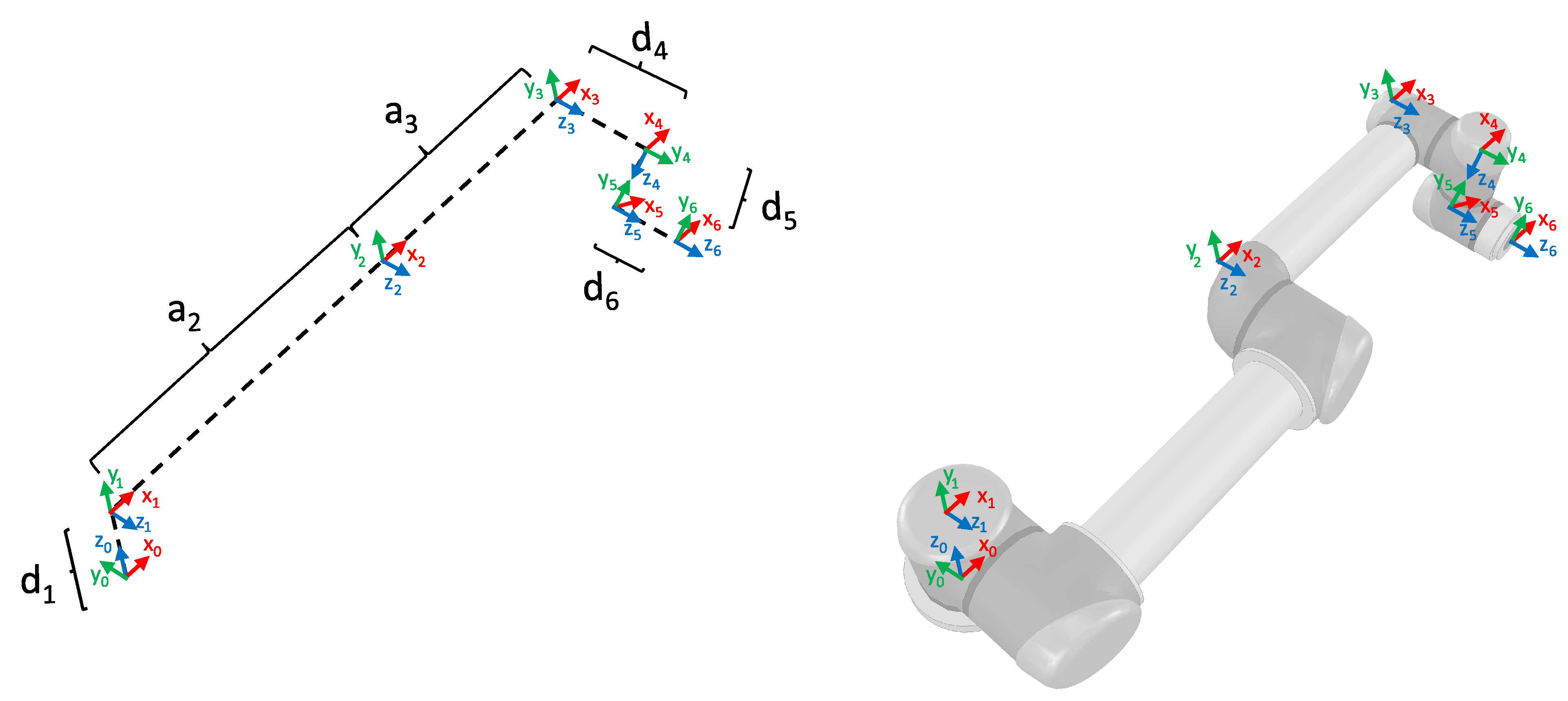
The UR5, which is the specific robot that was used for the experiments, is a 6-degree-of-freedom (DOF) cobot that only has rotational joints.
Table 1 presents its DH parameters, which are illustrated in
Figure 1. However, the IK solution and the singularity analysis only use variables, because this allows for using them for any other robot with the same geometry.
From the different IK solutions found in the literature, only one was considered to define the algorithms presented here; however, these algorithms can be easily modified to use a solution that calculates the angles in a different order. The following notation is used in this work:
,
,
and
. The homogeneous transformation matrix from Equation (
1) is composed of a rotational submatrix (elements represented by
r) and a position vector (
p elements); these define the orientation and position of frame 6 with respect to the base (frame 0). Since the DK solution is required to compute the IK solution, the resulting transformation matrix and its elements are shown next [
10]:
Although some equations are expressed differently, the IK solution used in this work consists of the following expressions that were proposed in [
8]:
2.2. Singularities
The Jacobian is a matrix that relates the joint velocities to the linear and angular velocities of the end effector. This matrix is used to find singularities because, for nonredundant robots such as the UR5, they exist when
; the Jacobian can be computed using different methods, one of which is shown in [
27].
In [
28], the authors mentioned that a robot is at a singularity or singular configuration when it is impossible to move the end effector in at least one direction; there, the Jacobian was computed as in Equations (
31) and (
32) for prismatic and rotational joints, respectively.
In the previous equations,
is the unit vector representing the
z-axis of joint
with respect to the base (frame 0),
is the end-effector position with respect to frame
, and
and
represent the parts of the Jacobian that relate the joint velocities to the linear and angular ones, respectively. An example of how the Jacobian matrix is computed using this method can be found in [
28].
Vectors and can be obtained from the DK study because is equal to (third column of rotational matrix ), and can be obtained by subtracting the translation vector from the end-effector position.
Since joint velocities tend to infinity as the robot approaches a singular configuration, studying and avoiding singularities is necessary to help in rendering the interaction between robot and user safer.
2.3. Singularity Analysis
Only Equation (
32) is necessary to compute the Jacobian because the UR5 consists exclusively of rotational joints. Adapting the Jacobian matrix with the corresponding UR5 parameters, the following can be expressed:
The previous results allow computing
as shown next:
As previously mentioned, to verify if the combination of joint angles results in a singularity, the determinant of the Jacobian matrix must be computed to determine if it is equal to or close to zero. This can be conducted with the following expression:
Three types of singularities (shoulder, wrist, and elbow) exist for this robot. Information about them can be found in [
20,
21], and they are briefly described next.
A shoulder singularity happens when the last factor in Equation (
46), which involves angles
,
, and
, is equal to zero. One example can be seen in
Figure 2, which shows that the end effector cannot be moved along
.
Wrist singularities exist when , which mathematically happens when or . This renders and parallel.
An elbow singularity is present when , which happens when or . This means that the arm is fully stretched or bent; however, only the former case is physically possible.
2.4. Algorithms to Select a Solution
This section presents two complete algorithms that can be used to select one set of angles that does not result in a singularity. In this work, angles close to 0 were considered to be 0, and angles close to were defined as ; was added or subtracted until the computed angle was within .
Not all values computed by the IK solutions are valid, i.e., some of them lead to computational errors. The cases in which this happens are described next:
Computed
angles are not acceptable if they are complex and no valid set can be computed. For the used IK solution, it is enough to validate the result of the square root in Equation (
20).
is not acceptable if it is complex or if
; since the IK solution uses atan2, only the latter validation is necessary. The value of the limit for
was chosen because if the other sines and cosines in Equation (
46) are equal to 1, it results in
, which can be considered equal to zero. The other reason was that although
, the computational tools do not always give the exact value, e.g., in MATLAB R2021a
; this means that the determinant is not always exactly 0.
The angles for are not valid if , or when either or is complex. For the used IK solution, it is enough to validate . The value defined for to be valid was obtained using the same considerations described previously for .
Angles and are not considered to be acceptable if ; the value of the limit was chosen because if and are both equal to 1 and this term is , then , which can be considered to be zero.
Lastly, a complete set of angles is not considered to be valid when the manipulator reaches the outer limit of its workspace, which happens when and . However, this leads to , which was already defined as not valid.
Modifications to the following algorithms may be necessary depending on the application and the order in which the IK solution that is used computes the angles. These algorithms do not consider the presence of obstacles.
2.4.1. Algorithm 1
The first algorithm computes all the sets of angles that take the end effector to a previously specified pose, and then selects the one that requires moving the joints the least overall.
To select a set of variables, some works maximize a cost function depending on the objective (avoiding singularities, joint limits, or obstacles) [
29] or find trajectories that do not include the mutation of any joint angles at
[
30]; however, this algorithm selects the set as in [
31], where the total joint displacement is minimized. Although something similar was performed in [
32], where the solution that minimized joint movement was selected, weights were used to prioritize moving smaller joints, which were assigned smaller weights.
Even though a specific selection criterion is used, depending on the objective, it is possible to change it without affecting the rest of the steps.
This algorithm consists of the following steps:
- (1)
Both solutions are computed, and complex angles are discarded.
- (2)
The previously obtained values for are used to compute . The sets containing values of that are not considered valid are rejected.
- (3)
is computed for the remaining sets.
- (4)
The values of are computed and verified. Again, the solutions with angles that are not acceptable are discarded.
- (5)
Lastly, and are computed, and the sets of angles that are not valid are rejected.
- (6)
The algorithm selects the solution with the minimal difference with respect to the current joint positions, which is computed with the following equations:
and
where
p refers to a previous value,
i to a joint, and
j to the computed set.
2.4.2. Algorithm 2
When there are two possible solutions for an angle, the second algorithm chooses the one that moves the specific joint less and verifies it does not result in a singularity. This is to compute only one complete set of angles that results in the desired pose.
This algorithm uses the FSM shown in
Figure 3; this technique was used because it is a comprehensible computational model. The FSM technique defines the steps that have to be followed to complete a specified sequential task; a state is triggered by an event or completion signal activated in the previous state. In the proposed FSM, each step computes one or two angles, selects the closest option (if two possibilities exist), and verifies if the chosen angles are valid. If a value is not acceptable, it is modified, and a previous state is triggered. In this case, the task is to compute and select angles that do not result in singular configurations.
The states are described next:
State 1: The values of are computed and verified, and the one closer to the previous is selected. If a valid is found, State 5 is next.
State 5: As for , the two possible angles for are computed and verified, and the one closer to the previous value is selected. If an acceptable is found, State 6 is next. Since the difference between the values of is the sign, only one of them is necessary for the validation. If the computed angles are not valid, State 5 is repeated using the other ; however, no solution exists if has already been changed.
State 6: Here, is computed. This is followed by State 3.
State 3: As for and , both values are computed and verified, and the one closer to the previous is selected; State 24 is run if an acceptable exists. Again, it is only necessary to verify one of the calculated angles; if is not valid, one of the following states is next:
- -
State 6: if has not been modified, the other value for is used.
- -
State 5: if has been changed and has not, the other possible angle for is tested.
- -
End: no set of angles exists if, after changing , both possibilities for result in unacceptable values for .
State 24: and are computed in this state; for this reason, it is called State 24. If the resulting set of angles is valid, the algorithm has found a solution (“End” is the next state); otherwise, one of the following states is run:
- -
State 24: if the value of has not been changed, it is modified, and the state is repeated.
- -
State 6: if both angles have been used and only one has been used, the other possible is tested.
- -
State 5: if has been changed and both options have been tested, but has not been modified. The other angle is used.
- -
End: if the manipulator cannot be taken to the desired pose even after changing , , and .
End: this last state is reached when a valid set of angles is found or if it is impossible to find one.
3. Results and Discussion
This section compares the results obtained with the algorithms presented in
Section 2.4.
For the comparison, the desired poses are shown in
Table 2 (only sets 7 and 9 do not result in singularities). However, to choose a set of angles for said poses, the previous ones were assumed to be
.
Both algorithms were programmed in MATLAB R2021a. Other results can be obtained depending on how the algorithms and IK solutions are programmed (e.g., if values close to are defined as and not as , or if the joint angles are not limited to be within ).
Table 3 and
Table 4 present the sets of angles selected by Algorithms 1 and 2, respectively. Different results were chosen only in three tests (7, 8, and 9).
Table 5 shows the computed determinants and proves that the final sets did not result in singular configurations.
Table 6 presents the differences between the selected angles and the previous ones; these were computed as in Algorithm 1 using Equation (
48) and prove that Algorithm 2 sometimes chose a set that required moving the joints more than Algorithm 1.
3.1. Discussion
The results show that the algorithms did not always choose the same angles. However, selecting any of the computed sets that did not result in a singularity render it safer for the user to interact with the robot.
Although Algorithm 1 selected the angles that moved the robot the least, which means that the robot would reach the desired pose faster, Algorithm 2 would not lead to abrupt movements, which is even safer for the user.
It is recommended to use Algorithm 1 when it is necessary to choose the set of angles that moves the joints the least; however, the memory of the device used to compute the IK solution should be enough to store up to eight possibilities. Algorithm 2 is suggested for applications using devices with low computational resources and when the new configuration does not need to be as similar as possible to the previous one.
The derived expression and proposed methods to compute the determinant of the Jacobian require fewer parameters and calculations than the ones found in other works; this implies a computational advantage particularly useful for real-time applications. The proposed methods need modifications to use the solution in [
20]. Even though it is possible to use the equation in [
21] in the proposed algorithms, the determinant does not result in zero when either
or
is equal to
; these mathematical singularities exist and can be detected with Equation (
46).
3.2. Applications
A complete IK solution that avoids singularities is helpful in different applications; one of them is robot design, particularly to implement the inverse kinematic control of a robot with the same geometry. Other more advanced applications include image-based visual servoing and the control of robotic digital twins.
Image-based visual servoing, as seen in
Figure 4, refers to the use of features extracted from images to move the robot to a desired feature or pose. In the latter case, it is necessary to include the IK solution as a part of an external controller to choose one set of angles that can move the end effector as desired while avoiding singularities.
Using a digital twin as supervisory control of a physical robot requires the IK solution to be implemented in the digital twin controller to verify that the physical system is working as expected and under safe conditions, which is particularly important for cobots. The proposed validated IK solution that uses the FSM is suitable because it avoids abrupt changes in the joint motion, this also renders the system safer because joint velocities can be safely controlled if singularities can be detected and avoided.
4. Conclusions
Inverse kinematic solutions can be used to control real and virtual robots. However, when an IK solution is used, it is also necessary to consider the robot’s singular configurations to have complete and validated robot control algorithms. For that reason, this study used the Jacobian matrix of the UR5 robot and its determinant; the latter was used in two algorithms to select a set of angles that takes the robot to the desired pose without resulting in a singularity. In this way, the main contribution of this work is the definition of two alternative methods for the complete and validated computational implementation of IK solutions for the UR5 robot. Since reaching singularities leads to faster joint velocities, methods that help in avoiding singular configurations and in making it safer for people to interact with this kind of robot are essential additions to the IK solution and can be considered to be enhanced alternative inverse IK solutions for robotic arms with the UR geometry.
The results show that, although the two algorithms could lead to the same set of angles, this is not always true, which means that one of the presented algorithms can be more suitable depending on the application. For example, if one objective is to reach the desired pose faster, Algorithm 1 can be used to ensure that the set of angles that requires moving the joints the least overall is selected; however, by using an FSM and not computing all the possibilities, Algorithm 2 requires less storage space, which means that it can be used in devices with low computational resources; this algorithm also avoids abrupt joint movements.
As a final remark, the FSM-based method complements the IK solution procedure with advantages in the number of computations and performance by producing results that would not move the joints abruptly, which is desired for collaborative robots, and this method is helpful when using devices with low computational resources.
Future work will focus on using the IK solution and one of the selection algorithms to control a virtual UR5 that will later be used to control a physical UR5 robot. The chosen algorithm will be modified to select the set of angles that consumes the least power or to evaluate which one results in the trajectory that moves the robot as far as possible from singularities.
Author Contributions
Conceptualization, J.V., I.Y.S. and F.M.; Data curation, J.V.; Formal analysis, J.V.; Investigation, J.V.; Methodology, J.V.; Project administration, J.V. and F.M.; Resources, J.V., I.Y.S. and F.M.; Software, J.V.; Supervision, F.M.; Validation, J.V.; Visualization, J.V.; Writing—original draft, J.V.; Writing—review & editing, I.Y.S. and F.M.. All authors have read and agreed to the published version of the manuscript.
Funding
This research was funded by Consejo Nacional de Ciencia y Tecnología grant number (doctoral scholarship) 752557.
Institutional Review Board Statement
Not applicable.
Informed Consent Statement
Not applicable.
Data Availability Statement
Not applicable.
Conflicts of Interest
The authors declare no conflict of interest.
References
- Park, H.; Easwaran, A.; Andalam, S. TiLA: Twin-in-the-loop architecture for cyber-physical production systems. In Proceedings of the 2019 IEEE 37th international conference on computer design (ICCD), Abu Dhabi, United Arab Emirates, 17–20 November 2019. [Google Scholar] [CrossRef]
- Zhang, D.; Wei, B. A review on model reference adaptive control of robotic manipulators. Annu. Rev. Control 2017, 43, 188–198. [Google Scholar] [CrossRef]
- Analytic Inverse Kinematics for the Universal Robots UR-5/UR-10 Arms. Available online: https://smartech.gatech.edu/handle/1853/50782 (accessed on 24 October 2022).
- Supplementary Material: An Ultrasound Robotic System Using the Commercial Robot UR5. Available online: https://www.researchgate.net/publication/292987030_Supplementary_Material_An_Ultrasound_Robotic_System_Using_the_Commercial_Robot_UR5 (accessed on 24 October 2022).
- Kinematics of a UR5. Available online: https://rasmusan.dk/wp-content/uploads/ur5_kinematics.pdf (accessed on 24 October 2022).
- Liu, Q.; Yang, D.; Hao, W.; Wei, Y. Research on kinematic modeling and analysis methods of UR robot. In Proceedings of the 2018 IEEE 4th Information Technology and Mechatronics Engineering Conference (ITOEC), Chongqing, China, 14–16 December 2018. [Google Scholar] [CrossRef]
- Kebria, P.M.; Al-Wais, S.; Abdi, H.; Nahavandi, S. Kinematic and dynamic modelling of UR5 manipulator. In Proceedings of the 2016 IEEE International Conference on Systems, Man, and Cybernetics (SMC), Budapest, Hungary, 9–12 October 2016. [Google Scholar] [CrossRef]
- Villalobos, J.; Sanchez, I.Y.; Martell, F. Alternative Inverse Kinematic Solution of the UR5 Robotic Arm. In Advances in Automation and Robotics Research; Moreno, H.A., Carrera, I.G., Ramírez-Mendoza, R.A., Baca, J., Banfield, I.A., Eds.; Springer: Cham, Switzerland, 2022; pp. 200–207. [Google Scholar] [CrossRef]
- Zhao, R.; Shi, Z.; Guan, Y.; Shao, Z.; Zhang, Q.; Wang, G. Inverse kinematic solution of 6R robot manipulators based on screw theory and the Paden–Kahan subproblem. Int. J. Adv. Robot. Syst. 2018, 15, 1–11. [Google Scholar] [CrossRef]
- Villalobos, J.; Sanchez, I.Y.; Martell, F. Statistical comparison of Denavit–Hartenberg based inverse kinematic solutions of the UR5 robotic manipulator. In Proceedings of the 2021 International Conference on Electrical, Computer, Communications and Mechatronics Engineering (ICECCME), Mauritius, Mauritius, 7–8 October 2021. [Google Scholar] [CrossRef]
- Schreiber, L.-T.; Gosselin, C. Determination of the Inverse Kinematics Branches of Solution Based on Joint Coordinates for Universal Robots–Like Serial Robot Architecture. J. Mech. Rob. 2022, 14, 034501. [Google Scholar] [CrossRef]
- Wang, H.; Qi, H.; Xu, M.; Tang, Y.; Yao, J.; Yan, X.; Li, M. Research on the relationship between classic Denavit–Hartenberg and modified Denavit–Hartenberg. In Proceedings of the 2014 seventh international symposium on computational intelligence and design, Hangzhou, China, 13–14 December 2014. [Google Scholar] [CrossRef]
- Kohli, D.; Osvatic, M. Inverse kinematics of general 6R and 5R, P serial manipulators. J. Mech. Des. 1993, 115, 922–931. [Google Scholar] [CrossRef]
- Raghavan, M.; Roth, B. Inverse kinematics of the general 6R manipulator and related linkages. J. Mech. Des. 1993, 115, 502–508. [Google Scholar] [CrossRef]
- Manocha, D.; Canny, J.F. Efficient inverse kinematics for general 6R manipulators. IEEE Trans. Rob. Autom. 1994, 10, 648–657. [Google Scholar] [CrossRef]
- Husty, M.L.; Pfurner, M.; Schröcker, H.-P. A new and efficient algorithm for the inverse kinematics of a general serial 6R manipulator. Mech. Mach. Theory 2007, 42, 66–81. [Google Scholar] [CrossRef]
- Xin, S.Z.; Feng, L.Y.; Bing, H.L.; Li, Y.T. A simple method for inverse kinematic analysis of the general 6R serial robot. J. Mech. Des. 2007, 129, 793–798. [Google Scholar] [CrossRef]
- Qiao, S.; Liao, Q.; Wei, S.; Su, H.-J. Inverse kinematic analysis of the general 6R serial manipulators based on double quaternions. Mech. Mach. Theory 2010, 45, 193–199. [Google Scholar] [CrossRef]
- Wang, J.; Lu, C.; Zhang, Y.; Sun, Z.; Shen, Y. A numerically stable algorithm for analytic inverse kinematics of 7-degrees-of-freedom spherical-rotational-spherical manipulators with joint limit avoidance. J. Mech. Rob. 2022, 14, 051005. [Google Scholar] [CrossRef]
- FarzanehKaloorazi, M.H.; Bonev, I.A. Singularities of the typical collaborative robot arm. In Proceedings of the International Design Engineering Technical Conferences and Computers and Information in Engineering Conference, Quebec, Canada, 26–29 August 2018. [Google Scholar] [CrossRef]
- Weyrer, M.; Brandstötter, M.; Husty, M. Singularity avoidance control of a non–holonomic mobile manipulator for intuitive hand guidance. Robotics 2019, 8, 14. [Google Scholar] [CrossRef]
- Geometric Jacobians Derivation and Kinematic Singularity Analysis for Smokie Robot Manipulator & the Barrett WAM. Available online: https://arxiv.org/abs/1707.04821 (accessed on 24 October 2022).
- Development of Direct Kinematics and Workspace Representation for Smokie Robot Manipulator & the Barret WAM. Available online: https://arxiv.org/abs/1707.04820 (accessed on 24 October 2022).
- Pires, F.; Melo, V.; Almeida, J.; Leitão, P. Digital twin experiments focusing virtualisation, connectivity and real-time monitoring. In Proceedings of the 2020 IEEE Conference on Industrial Cyberphysical Systems (ICPS), Tampere, Finland, 10–12 June 2020. [Google Scholar] [CrossRef]
- Gao, C.; Piao, X.; Tong, W. Optimal motion control for IBVS of robot. In Proceedings of the 10th World Congress on Intelligent Control and Automation, Beijing, China, 6–8 July 2012. [Google Scholar] [CrossRef]
- Xiao, Y.; Fan, Z.; Li, W.; Chen, S.; Zhao, L.; Xie, H. A manipulator design optimization based on constrained multi-objective evolutionary algorithms. In Proceedings of the 2016 International Conference on Industrial Informatics-Computing Technology, Intelligent Technology, Industrial Information Integration (ICIICII), Wuhan, China, 3–4 December 2016. [Google Scholar] [CrossRef]
- Craig, J.J. Introduction to Robotics: Mechanics and Control, 3rd ed.; Pearson Prentice Hall: Hoboken, NJ, USA, 2005; pp. 135–159. [Google Scholar]
- Asada, H.; Slotine, J.-J.E. Robot Analysis and Control, 1st ed.; John Wiley & Sons: New York, NY, USA, 1986; pp. 51–71. [Google Scholar]
- Zaplana, I.; Basanez, L. A novel closed-form solution for the inverse kinematics of redundant manipulators through workspace analysis. Mech. Mach. Theory 2018, 121, 829–843. [Google Scholar] [CrossRef]
- Gong, M.; Li, X.; Zhang, L. Analytical inverse kinematics and self-motion application for 7-DOF redundant manipulator. IEEE Access 2019, 7, 18662–18674. [Google Scholar] [CrossRef]
- Kalra, P.; Mahapatra, P.B.; Aggarwal, D.K. An evolutionary approach for solving the multimodal inverse kinematics problem of industrial robots. Mech. Mach. Theory 2006, 41, 1213–1229. [Google Scholar] [CrossRef]
- Tong, Y.; Liu, J.; Liu, Y.; Yuan, Y. Analytical inverse kinematic computation for 7-DOF redundant sliding manipulators. Mech. Mach. Theory 2021, 155, 104006. [Google Scholar] [CrossRef]
- Corke, P.I. Visual Control of Robots: High-Performance Visual Servoing; Research Studies Press: Taunton, UK, 2005; pp. 152–154. [Google Scholar]
| Publisher’s Note: MDPI stays neutral with regard to jurisdictional claims in published maps and institutional affiliations. |
© 2022 by the authors. Licensee MDPI, Basel, Switzerland. This article is an open access article distributed under the terms and conditions of the Creative Commons Attribution (CC BY) license (https://creativecommons.org/licenses/by/4.0/).


